[NORMAL] Jrdf Algorithm for Joint Range-DOA-Frequency Estimation of Mixed Near-Field and Far-Field Sources

JRDF Algorithm for Joint Range-DOA-Frequency Estimation

of Mixed Near-Field and Far-Field Sources

Fulai Liu1, 2, *, Jian Ma1, 2, and Ruiyan Du1, 2

Abstract—This paper presents an effective joint range-DOA-frequency (JRDF) estimation method based on fourth-order cumulants for multiple mixed near-field sources and far-field sources impinging on a symmetric uniform linear array, named as JRDF algorithm. Making use of the proposed method, range-DOA-frequency can be effectively estimated by the same eigen-pair of a defined “information matrix” constructed by two fourth-order cumulant matrices. Compared with the related works, the proposed method can provide superior performance, such as higher estimation accuracy, without the procedure of parameter search or parameter matching. Simulation results are presented to demonstrate the efficacy of the proposed approach.

1. INTRODUCTION

Source localization from noisy observations is one of the fundamental problems in array signal processing, such as sonar, radar, seismic exploration system and microphone arrays [1]. Therefore, it has received a significant amount of attention, and a number of algorithms have been developed to deal with far-field sources (FFSs) [2–5] or near-far-field sources (NFSs) [6–9]. For FFSs (beyond Fresnel zone) scenario, the wavefronts are usually approximated as planar, thus only DOA parameter needs to be estimated when the carrier frequency is known. Otherwise, for the NFSs (in Fresnel zone), as the wavefronts are spherical, both DOA and range parameters should be estimated when the carrier frequency is known as a priori. In some practical applications, the signals received at an array may be the mixture of NFSs and FFSs, for example, when using microphone arrays to localize speakers’ localizations, each speaker may be in near-field (NF) or far-field (FF) since speakers’ positions keep changing. So the pure NF source localization and pure FF source localization algorithm may encounter problems in localizing mixed NFSs and FFSs.

Recently, several high resolution methods have been presented to resolve the parameter estimation problem for the mixed NFSs and FFSs [10–17]. A two-stage MUSIC algorithm using cumulant is presented to solve the mixed source localization [10]. Despite its effectiveness, this algorithm has a high computational burden since it involves multiple eigenvalue decompositions for high order cumulant matrices and one-dimensional (1-D) MUSIC spectrum peak search. To decrease its computational burden, an efficient application of MUSIC algorithm based on second order statics is proposed in [11]. It requires neither a multidimensional search nor high-order statics. Unfortunately, this method has loss of array aperture. Via ESPRIT-Like and polynomial rooting methods, an effective mixed sources localization algorithm is given in [12]. It can obtain better estimation performance and lower computational cost. A two-stage matrix differencing algorithm is derived to classify and locate mixed NF and FF sources [13]. This method not only improves estimation accuracy, but also achieves a more reasonable classification of the signal types. Du et al. present a space-time matrix to localize mixed

Received 18 May 2015, Accepted 23 July 2015, Scheduled 9 August 2015

* Corresponding author: Fulai Liu ([email protected]).

1 _{Engineer Optimization & Smart Antenna Institute, Northeastern University at Qinhuangdao, China.} 2 _{School of Information}

NFSs and FFSs [14]. By using this method, both the DOAs and ranges of sources can be estimated by the same eigen-pair of a defined space-time matrix which avoids parameter matching problems. An improved mixed source localization method based on sparse signal reconstruction is proposed in [15]. This method firstly transforms the time-domain data of array into cumulant domain data to estimate DOAs, then constructs the mixed overcomplete basis to get the sparse representation of the array output for range estimation. It can resolve the closely spaced source and provide higher estimation accuracy. A mixed-order MUSIC algorithm for NF and FF sources localization using a sparse symmetric array is proposed in [16]. This method constructs a cumulant matrix to estimate DOAs of the mixed sources by exploiting the special array geometry. Via a crossed array, a three-dimensional (3-D) mixed NF and FF sources localization algorithm is presented in [17]. As it is based on second order statistics and requires 1-D search, it has low computational burden. In addition, it is able to avoid parameter pairing procedure as well.

To decrease the computational burden and avoid parameters pairing, a JRDF estimation algorithm is proposed to resolve the mixed source localization problem when NFSs and FFSs coexist. The ranges, DOAs and frequencies of all incoming signal sources can be estimated by the eigen-pair of a defined “information matrix” based on fourth-order cumulants. The outline of this paper is organized as follows. Section 2 briefly introduces data model. The JRDF estimation algorithm is described in Section 3. Section 4 shows several simulation results to verify the performance of the proposed approach. Finally, Section 5 provides a concluding remark to summarize the paper.

2. DATA MODEL

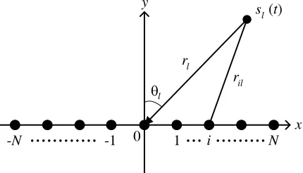
Consider the receiving system with uniform linear array (ULA) (shown in Fig. 1) which consists of 2N + 1 isotropic sensors. Assume that there are L independent narrowband sources impinging on the ULA from NF or FF.

0 x

y

l

r

θ

l

r_il s _l(t)

-1

-N

...

... ...

Figure 1. Uniform linear array configuration.

Employ the centre of the array as the phase reference point. Assume that there areLnarrowband sources of interest, with complex baseband representations sl(t), for l = 1,2, . . . , L. Suppose that the

lth source has a carrier frequency of fl. The signal received at theith antenna is

xi(t) = L

l=1

sl(t)ej2πfltejτil+ni(t) (−N ≤i≤N) (1)

wherexi(t) and ni(t) denote the output and the additive noise output of theith sensor.

As θl and rl are the DOA and range of the lth source relative to the phase reference point, respectively, the distance ril from the lth source to the ith sensor is given by a simple application of the law of cosines

ril =

r2

l + (id)2−2rlidcos _π

2 −θl

−N ≤i≤N (2)

The delay τil, which is associate with the lth source signal propagation time between the phase reference point and theith sensor, can be expressed as

τil= 2π(ril−rl)

λl (3)

thus using the Fresnel approximation [18], (3) can be approximated as

ˆ

τil≈i−2πd

λl sin(θl) +i 2πd2

λlrlcos 2_(θ

l) (4)

For NFSs, rl is restricted to the Fresnel zone. They must be characterized by both the azimuth DOA and range, because the wavefronts are spherical. For FFSs,rl is far beyond the Fresnel zone, so we can treat spherical wavefronts as planar wavefronts (plane-wave approximation) when they propagate across the array. When this approximation is substituted into (4), the phase of the delay term becomes a linear function as follows

ˆ

τil ≈i−2πd

λl sin(θl) (5) Therefore, FF can be regarded as a special case of the NF.

In addition, the parameters γl and φl are the functions of the azimuth θl and range rl of the lth source

γl=−2_λπd

l sin(θl) (6)

and

φl = πd 2

λlrl cos 2₍

θl) (7)

whereθl∈[−π/2, π/2], rl∈[0.62(D2/λl)1/2,+∝), Drepresents the array aperture.

After being sampled with a proper ratefs that satisfies the Nyquist rate, the data sampleX(k) at the receiver is

X(k) =AS(k) +N(k) (k= 1,2, . . . , K) (8) where X(k) = [x_−N(k), . . . ,x0(k), . . . ,xN(k)]T is the array output matrix. S(k) = [s1(k)ejω1k, s2(k)ejω2k, . . . , sL(k)ejωLk]T represents the signal waveform vector. The normalized radian frequency ωl = 2πfl_fs . λl = _flc = _ωlfs2πc. N(k) = [n−N(k), . . . , n0(k), . . . , n+N(k)]T stands for the noise vector. K stands for the snapshot number. A= [a(θ1, r1),a(θ2, r2), . . . ,a(θL, rL)] is the (2N + 1)×L array steering matrix of the mixed NFSs and FFSs. The array steering vector can be given as

a(θl, rl) =

ej[(−N)γl+(−N)2φl], . . . , ej[(−i)γl+(−i)2φl], 1, ej[iγl+i2φl], . . . , ej[Nγl+N2φl]

_T

(9)

where the superscript (·)T stands for the matrix transpose. rl ∈ [0.62(D2/λl)1/2,2D2/λl] ∪ (2D2/λl,+∝).

The common assumptions are listed as follows

(A1) The source signals are mutually independent, non-Gaussian, narrowband stationary processes with nonzero kurtosis.

(A2) The sensor noise is zero-mean (white or colored) Gaussian signals and independent of the source signals.

(A3) The array is a ULA with element spacingdmin(λl/4).

(A4) The array is a symmetric array with 2N + 1 sensors and the source number L < 2N + 1 is assumed.

(A5) The wavelength parameters of the sources are different from each other, that is ωi =ωj for

3. ALGORITHM FORMULATION

To develop an efficient joint estimation algorithm, we define a fourth-order cumulant matrix C1, the (m, n)th element of which is defined as

C1(m, n) = cum

x0(k),x0∗(k),xm−N−1(k),x∗_n−N−1(k) (10) where the superscript (·)∗ represents the complex conjugate. Substituting (8) into (10) and using the multilinearity property of cumulant together with the assumptions (A1) and (A2), we can get C1 as follows

C1(m, n) = L

l=1

c4,slej{(m−n)γl+[(m−N−1)

2_{−(n−N−1)}2_]φl} =

L

l=1

c4,slej{(m−N−1)γl+(m−N−1)

2_φl}

×ej{(n−N−1)γl+(n−N−1)2φl}

_∗

(m, n∈[1,2N + 1]) (11)

where c4,sl = cum{|sl(t)|4} denotes the kurtosis of sl(t). Let C4s = diag{c4,s1, c4,s2, . . . , c4,sL} be a diagonal matrix composed of the source kurtosis, thus we have

C1 = BC4sBH (12)

B = [b(γ1),b(γ2), . . . ,b(γl), . . . ,b(γL)] (13)

b(γl) =

ej[(−N)γl+(−N)2φl], . . . ,1, . . . , ej[Nγl+N2φl]

_T

(l= 1, . . . , L) (14)

where the superscript (·)H denotes Hermitian transpose.

Since all source signals are assumed to have nonzero kurtosis,C4s is an invertible diagonal matrix. Additionally, rank(B) =L, hence, C1 is a (2N+ 1)×(2N+ 1) matrix with rank L.

Furthermore, for different sensor lags, we define

C2(m, n) = cum

x0(k+ 1),x∗0(k),xm−N−1(k),x∗_n−N−1(k) (m, n∈[1,2N + 1]) (15) and under the narrow-band assumption, we havesl(k+ 1)≈sl(k).

Similar to (12),C2 has the following expression

C2 =BΩC4sBH (16)

and

Ω= diagejω1_{, e}jω2_{, . . . , e}jωL ₍₁₇₎

It is easy to know thatC2 is also a (2N+ 1)×(2N+ 1) matrix with rank L.

Let P = diag{ρ1, ρ2, . . . , ρ2N+1} and V = [v1,v2, . . . ,v2N+1] be the eigenvalues and the corresponding eigenvectors ofC1, then we can get

C1= 2N+1

l=1

ρlvlvHl =VPVH =VsPsVsH+VnPnVHn (18)

where P = diag{ρ1, ρ2, . . . , ρ2N+1} with ρ1 ≥ ρ2 ≥ . . . ≥ ρL > ρL+1 = . . . = ρ2N+1 = 0.

V = [V_sV_n]. V_s = [v1,v2, . . . ,vL], Ps = diag{ρ1, ρ2, . . . , ρL}, Vn = [vL+1,vL+2, . . . ,v2N+1] and

P_n= diag{ρL+1, ρL+2, . . . , ρ2N+1}. Similarly, defineC3 as follows

C3= L

l=1 1

ρlvlv H

l =VsPs−1VHs (19)

From (12) and (18), it is easy to know that the signal subspaceV_s concides with the range space of B. Since span{V_s}= span{B}, there must exist a unique invertible matrix T, such that B=V_sT. Therefore, it holds that

Making use of C2 and C3, define an “information matrix” C (which includes the information of DOAs, ranges and frequencies) as following

C=C2C3 (21)

Then we have the following Theorem.

Theorem 3.1. Assume that there are L (near-field or far-field) narrow-band sources, with the complex baseband representations sl(t)(1 ≤l≤L) such that the lth source has a carrier frequency fl and arrives a ULA from directionθl, rangerl. If there are no same elements on the diagonal of matrix

Ω, then, theL largest nonzero eigenvalues of Care equal to theL elements on the diagonal of matrix

Ω, and the corresponding eigenvectors are equal to the corresponding column vectors of B, namely

CB=BΩ.

Proof: Under the above assumption, it is easy to know thatB is a full rank matrix. Furthermore, we draw a conclusion that rank(B) = rank(C) = L. From (12), (16) and (18)∼(20), the following equation can be obtained

CB = C2C3B=BΩC4sBHVsP−_s1VH_s B=BΩ

BHB−1BHBC4sBH

V_sP−_s1VH_s B

= BΩBHB−1BHC1VsP−_s1V_sHB=BΩ

BHB−1BHV_sP_sVH_s V_sP−_s1VH_s B

= BΩBHB−1BHV_sVH_s B=BΩBHB−1BHB=BΩ (22)

where the superscript (·)−1 denotes matrix inverse. This concludes the proof.

Remarks:

(1) From Theorem 3.1, it can be easily seen that the array response matrix B and the diagonal matrix Ωcan be obtained by computing the eigendecomposition of the “information matrix” C. The following incoming angleθl, rangerl and frequencyfl can be estimated by making use of thelth eigen-pair of the matrix C, that is, the paring of the estimated 3-D parameters is automatically determined. (2) If there are several sources close in the angle of incidence θ or range r, but there are no same elements on the diagonal of matrixΩ, then Theorem 3.1 is still true, namely, it can resolve the incoming rays with very close angles or very close ranges under the aforementioned conditional restriction.

Meanwhile,Ccan be decomposed into

C= 2N+1

l=1

αluluHl =UΛUH =UsΛsUHs +UnΛnUHn (23)

where Λ = diag{α1, α2, . . . , α2N+1} with α1 ≥ α2 ≥ . . . ≥ αL > αL+1 = . . . = α2N+1 = 0.

U = [U_sU_n]. U_s = [u1,u2, . . . ,uL], Λs = diag{α1, α2, . . . , αL}, Un = [uL+1,uL+2, . . . ,u2N+1] and

Λ_n= diag{αL+1, αL+2, . . . , α2N+1}.

From (23), it is easy to see that ejωl and b(γl) (l = 1,2, . . . , L) are just the eigenvalue and corresponding eigenvector of C. Based on (13), (14), (22) and (23),fl and b(γl) can be given by

fl= angle(_2παl)fs (24)

and

b(γl) = ul

u_l[N + 1] (25)

where the angle(·) denotes the phase angle operator.

To facilitate the representation, let b_l take the place of b(γl) and the ith element of bl can be expressed asb_l(i), thus from (13) and (14), it has the following form

b_l(i) =ej[(−N−1+i)γl+(−N−1+i)2φl] (26) By using (26),d_l(i) and e_l(i) have the following expression

d_l(i) = b_l(i+ 1)b∗_l(i)b∗_l(3)b_l(2)

= ej[(−N+i)γl+(−N+i)2φl]e−j[(−N+i−1)γl+(−N+i−1)2φl]

and

e_l(i) = b_l(i+ 1)b∗_l(i)b∗_l(2N −1)b_l(2N)

= ej[(−N+i)γl+(−N+i)2φl]e−j[(−N+i−1)γl+(−N+i−1)2φl]

e−j[(N−2)γl+(N−2)2φl]ej[(N−1)γl+(N−1)2φl]=ej[2(i−2)φl+2γl] (28) Based on b_l, we can form two 2N-dimensional column vectors as follows

d_l= ⎡ ⎢ ⎢ ⎢ ⎢ ⎢ ⎢ ⎣

b_l(2)b∗_l(1)b∗_l(3)b_l(2)

b_l(3)b∗_l(2)b∗_l(3)b_l(2) ..

.

b_l(2N −1)b∗_l(2N −2)b∗_l(3)b_l(2)

b_l(2N)b∗_l(2N −1)b∗_l(3)b_l(2)

b_l(2N+ 1)b∗_l(2N)b∗_l(3)b_l(2) ⎤ ⎥ ⎥ ⎥ ⎥ ⎥ ⎥ ⎦ = ⎡ ⎢ ⎢ ⎢ ⎢ ⎢ ⎢ ⎢ ⎣

ej(−2)φl

1 .. .

ej(4N−8)φl ej(4N−6)φl ej(4N−4)φl

⎤ ⎥ ⎥ ⎥ ⎥ ⎥ ⎥ ⎥ ⎦ (29) and

e_l= ⎡ ⎢ ⎢ ⎢ ⎢ ⎢ ⎢ ⎣

b_l(2)b∗_l(1)b_l∗(2N −1)b_l(2N)

b_l(3)b∗_l(2)b_l∗(2N −1)b_l(2N) ..

.

b_l(2N −1)b∗_l(2N−2)b∗_l(2N −1)b_l(2N)

b_l(2N)b∗_l(2N −1)b∗_l(2N −1)b_l(2N)

b_l(2N + 1)b∗_l(2N)b∗_l(2N −1)b_l(2N) ⎤ ⎥ ⎥ ⎥ ⎥ ⎥ ⎥ ⎦ = ⎡ ⎢ ⎢ ⎢ ⎢ ⎢ ⎢ ⎢ ⎣

ej[(−2)φl+2γl] ej[2γl]

.. .

ej[(4N−8)φl+2γl]

ej[(4N−6)φl+2γl] ej[(4N−4)φl+2γl]

⎤ ⎥ ⎥ ⎥ ⎥ ⎥ ⎥ ⎥ ⎦ (30)

Based on d_l and e_l,{γl, φl} can be given by

γl= 1 4N

2N

i=1

e_l(i)

d_l(i) (31)

and

φl= _8N1_{−4 2N−1}

i=1 arg

d_l(i+ 1)

d_l(i)

+ 2N−1

i=1 arg

e_l(i+ 1)

e_l(i)

(32)

The wavelength of thelth sourceλlis easily obtained fromfl. According to (6), (7), (31) and (32), the azimuth and range estimation of the lth source can be in turn expressed as

θl= arcsin

−γlλl

2πd

(33)

and

rl= πd 2

λlφl cos 2₍

θl) (34)

In fact, according to (34), we can easily determine that the lth source is a NF or FF one. When

rl ∈ [0.62(D2/λl)1/2,2D2/λl] (Fresnel region), we can determine that the lth source corresponding to

rl is a NF source. On the contrary, when rl ∈ (2D2/λl,+ ∝), we can determine that the lth source corresponding torl is a FF source.

4. SUMMARY OF JRDF

(1) Collect data and conduct two fourth-order cumulant matrices C1 and C2 denoting the estimate ˆC1 and ˆC2, respectively.

(2) Compute the eigendecomposition of ˆC1 and use its L maximum nonzero eigenvalues ˆPs = diag{ρˆ1, . . . ,ρˆL} and the corresponding eigenvectors ˆVs to define ˆC3 according to AIC [19], if L is unknown.

(4) Use theL maximum nonzero eigenvalues ˆΛ_s and its corresponding eigenvectors ˆU_s (the eigen-pairs ( ˆαl,uˆl), l = 1,2, . . . , L) of ˆCto estimate the frequency of thelth source ˆfland ˆblby (24) and (25), respectively.

(5) Estimate ˆd_l and ˆe_l by making use of ˆb_l from (29) and (30), respectively. (6) Implement ˆd_l and ˆe_l to estimate ˆγl and ˆφl by (31) and (32), respectively.

(7) The DOA and range estimations of thelth source can be in turn expressed as (33) and (34), respectively.

(8) Use the range estimation of the lth source ˆrl to determine whether the lth source is NFS or FFS.

Remarks:

(1) It is well known that the accuracy of the results is concerned with array aperture. When

τ 1/B (τ =D/c with Ddenoting the array aperture, c standing for the velocity of electromagnetic waves,Bbeing the incoming signal’s bandwidth, respectively), as the array aperture becomes larger, the accuracy of the results gets higher. Moreover, the array aperture is concerned with the number of the array’s elements and the distance between two adjacent array elements. As the number of the array’s elements and the distance between two adjacent elements become larger, the accuracy of the results grows higher. However, when d > λ/4 (d is the distance between two adjacent array elements and λ

equal to the wavelength), although the accuracy of the results improves, it will cause phase ambiguity. So the distance between two adjacent array elements is set to d=λ/4 .

(2) As the antenna array patterns may not be entirely consistent, it may cause gain-and-phase errors in the real world. In reality, the elements of the array should be calibrated according to the existing calibration methods such as active calibration [20] and self-calibration [21], etc.

(3) The source number estimation problem is an important problem in array signal processing, etc. Generally, the source number estimation is a prior. If the number is unknown, we can use AIC [19] (Akaike Information Criteria) and GDE [22] (Gerschgorin’s Disk Estimation) to detect the number of the incoming signals. However, this paper mainly focuses on the joint range-DOA-frequency estimation problem. The source number estimation problem may be beyond the scope of this paper.

5. COMPUTATIONAL COMPLEXITY

We briefly investigate the computational complexity of the proposed algorithm. The computational complexity of the proposed algorithm mainly includes: (1) fourth-order cumulants matrix construction of two P×P matrixes C1 and C2, respectively, of ordersO(9P2) (whereP = 2N + 1, Q= 4N + 1); (2) the eigendecomposition (EVD) of two P×P matrixes C1 andC, respectively, of orders O(4/3P3). Table 1 presents the complexity of the proposed method and the methods in [10]. For comparison, the method in [10] and the proposed method are named as TSMUSIC and JRDF, respectively.

Table 1. Comparison of the computational complexity of the proposed algorithm with TSMUSIC.

Algorithms construction of matrix EVD peak search

JRDF twiceO(9P2) twice O(4/3P3) without TSMUSIC ones O(9P2) ones O(4/3P3) ones

ones O(9Q2) ones O(4/3Q3)

6. SIMULATION RESULTS

λ2 = 100), radiate on the array. For comparison, we simultaneously execute the algorithm in [10] and the related CRB [23] (see Appendix for details) in the following experiments and figures. The frequency, DOA and range estimates are scaled in units of MHz, degree and wavelength. Assume that there are one NFS and one FFS and they are located at (10◦, λ1) and (20◦, 45λ2). The number of snapshots is N = 100. And the performance of these algorithms is measured by the estimated root mean-square error (RMSE) of 400 independent Monte Carlo runs. The RMSE_f, RMSE_θ and RMSE_r are defined as

follows _⎧ ⎪ ⎪ ⎪ ⎪ ⎪ ⎪ ⎪ ⎪ ⎪ ⎪ ⎪ ⎪ ⎪ ⎪ ⎪ ⎨ ⎪ ⎪ ⎪ ⎪ ⎪ ⎪ ⎪ ⎪ ⎪ ⎪ ⎪ ⎪ ⎪ ⎪ ⎪ ⎩

RMSE_f = _{E L} l=1

fl−fˆl 2

RMSE_θ = _{E L} l=1

θl−θˆl 2

RMSE_r= _{E L} l=1

(rl−rˆl)2

(35)

where ˆfl, ˆθl and ˆrl are the estimate of fl, θl and rl, for l= 1,2, . . . , L.

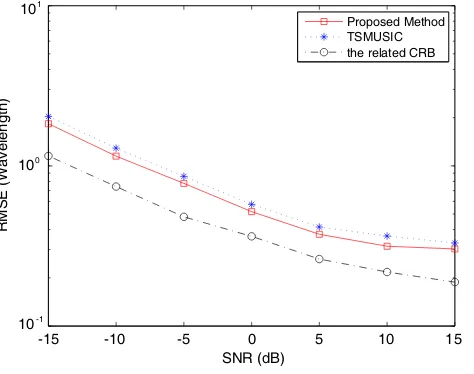
Figures 2, 3 and 4 give RMSE_f curves with SNR from−15 to 15 dB. The solid line stands for the RMSE curve of the proposed method. The dotted line represents the RMSE curve of TSMUSIC. The dotted and dash line shows the RMSE curve of the related CRB. Fig. 2 shows that JRDF estimation algorithm has high frequency estimation accuracy. By contrast, TSMUSIC method assumes that the carrier frequency is known as a priori. From Figs. 3 and 4, we can note that the proposed method outperforms TSMUSIC method in frequency, DOA and range estimates. In addition, the proposed method shows a more satisfactory performance than TSMUSIC and the RMSEs are reasonably close to the related CRB.

When SNR is set to 10 dB and the snapshot number varies from 50 to 500, RMSE_f curves of the JRDF and related CRB are shown in Fig. 5. In addition, the RMSE_θ and RMSE_r curves of the aforementioned two algorithms and related CRB are shown in Fig. 6 and Fig. 7, respectively. From Fig. 5, we can know that JRDF estimation algorithm has satisfactory frequency performance. However, TSMUSIC assumes that the carrier frequency is known as a priori. As shown in Fig. 6 and Fig. 7, the proposed method has higher estimation accuracy than that of TSMUSIC, and the curves of the proposed method are closer to the related CRB.

-15 -10 -5 0 5 10 15 10 -4

10 -3 10 -2 10 -1 100

SNR (dB)

RMSE (MHz)

Proposed Method the related CRB

Figure 2. RMSE_f curves versus SNR.

10 10 100 101 RMSE (degree) Proposed Method TSMUSIC the related CRB

-15 -10 -5 0 5 10 15

-2 -1

SNR (dB)

10 100

101

RMSE (Wavelength)

Proposed Method TSMUSIC the related CRB

-15 -10 -5 0 5 10 15 -1

SNR (dB)

Figure 4. RMSE_r curves versus SNR.

50 100 150 200 250 300 350 400 450 500 10 -3

10 -2 10 -1

Snapshot Number

RMSE (MHz)

Proposed Method the related CRB

Figure 5. RMSE_f curves versus snapshot number.

50 100 150 200 250 300 350 400 450 500 10

10 100 101

Snapshot Number

RMSE (degree)

Proposed Method TSMUSIC the related CRB

-2 -1

Figure 6. RMSE_θ curves versus snapshot number.

50 100 150 200 250 300 350 400 450 500 10

100 101

Snapshot Number

RMSE (Wavelength)

Proposed Method TSMUSIC the related CRB

-1

Figure 7. RMSE_r curves versus snapshot number.

7. CONCLUSIONS

In this paper, a JRDF estimation algorithm based on fourth-order cumulants is presented for mixed sources localization. Eigen-pairs of the defined “information matrix” are used to estimate the ranges, DOAs and frequencies. So the pairing of the estimated parameters is automatically determined. The presented approach has a lower computational complexity, but it exhibits superior performance, such as smaller estimation error and better robustness to SNR change.

ACKNOWLEDGMENT

Bureau of Education of Hebei Province, China, under Grant No. Z2011129, and by the National Natural Science Foundation of China under Grant No. 60904035, and by the Specialized Research Fund for the Doctoral Program of Higher Education of China (No. 20130042110003), and by Science and Technology Support Planning Project of Northeastern University at Qinhuangdao (XNK201302). The authors also gratefully acknowledge the helpful comments and suggestions of the reviewers, which have significantly improved the presentation of this paper.

APPENDIX A.

In this appendix, we derive the CRB for the estimated parameters [9]. By virtue of (8), we can get

ni(k) =xi(k)− L

l=1

sl(k)ejωlkej(iγl+i2φl) (A1)

From (A1), we define the probability density function p(x|ψ) as

p(x|ψ) = K

k=1 N

i=−N 1

√

2πσ2e

− 1 2σ2

xi(k)−L

l=1sl(k)e

jωlk_ej(_iγl+i2_φl)

H

xi(k)−L

l=1sl(k)e

jωlk_ej(_iγl+i2_φl)

(A2)

wherex= [x(1),x(2), . . . ,x(K)]T andψ= [ψ1, . . . , ψl, . . . , ψL]T. ψl can be expressed as follows

ψl= [ωl θl rl] (A3) The natural algorithm ofp(x|ψ) can be expressed as

ln(p(x|ψ)) = −1

2(2N + 1)Kln

2πσ2

− 1

2σ2 K

k=1 N

i=−N

xi(k)− L

l=1

sl(k)ejωlkej(iγl+i2φl) H

xi(k)− L

l=1

sl(k)ejωlkej(iγl+i2φl) (A4)

Based on (37), (38) and (39), the partial derivative respect to the three elements of ψl for the near-field or far-field sources can be respectively given by

∂ln(p(x|ψ))

∂ωl = 1 σ2 K k=1 N

i=−N !

Re

jksl(k)ejωlkej(iγl+i2φl)n∗_i(k) "

, (A5)

∂ln(p(x|ψ))

∂θl = 1 σ2 K k=1 N

i=−N #

Re $

jksl(k)ejωlkej(iγl+i2φl)

−2πdicosθl

λl −

πd2_i2_sin(2θ l)

λlrl

n∗_i(k) %&

, (A6)

∂ln(p(x|ψ))

∂rl = 1 σ2 K k=1 N

i=−N #

Re $

jksl(k)ejωlkej(iγl+i2φl)

−πd2i2cos2θl

r2 l

n∗_i(k) %&

(A7)

So the partial derivative with respect toψl for the near-filed and far-field sources can be expressed as follows

∂ln(p(x|ψ))

∂ψl = $

∂ln(p(x|ψ))

∂ωl

∂ln(p(x|ψ))

∂θl

∂ln(p(x|ψ))

∂rl %_T

(A8)

Based on (40)–(43), we obtain ∂ln(p_∂ψl(x|ψ)) for all L sources and then form the following column vector ∂ln(p_∂ψ(x|ψ)) by using ∂ln(p_∂ψl(x|ψ))

∂ln(p(x|ψ))

∂ψ =

$

∂ln(p(x|ψ))

∂ψ1 . . .

∂ln(p(x|ψ))

∂ψl . . .

∂ln(p(x|ψ))

∂ψL %_T

Based on (44), we obtain the Fisher informationF

F=E

∂ln(p(x|ψ))

∂ψ

∂ln(p(x|ψ))

∂ψ

_T

(A10)

So the CRB on the variance of the estimated parameters can be obtained from the related diagonal elements of the inverseF−1[20]. In this paper, the Fisher information matrixFis estimated by averaging the 400 computations of ∂ln(p_∂ψ(x|ψ))(∂ln(p_∂ψ(x|ψ)))T in the 400 independent Monte Carlo runs.

REFERENCES

1. Krim, H. and M. Viberg, “Two decades of array signal processing research: The parametric approach,”IEEE Transactions on Signal Processing Magazine, Vol. 13, No. 4, 67–94, 1996. 2. Schmidt, R. O., “Multiple emitter location and signal parameter estimation,” IEEE Transactions

on Antennas and Propagation, Vol. 34, No. 3, 276–280, 1986.

3. Roy, R. and T. Kailath, “ESPRIT-estimation of signal parameters via rotational invariance techniques,” IEEE Transactions on Acoustics, Speech and Signal Processing, Vol. 37, No. 7, 984– 995, 1989.

4. Gao, F. and A. B. Gershman, “A generalized ESPRIT approach to direction-of-arrival estimation,” IEEE Signal Processing Letters, Vol. 12, No. 3, 254–257, 2005.

5. Liu, F. L., J. K. Wang, and C. Y. Sun, “Spatial differencing method for DOA estimation under the coexistence of both uncorrelated and coherent signals,” IEEE Transactions on Antennas and Propagation, Vol. 60, No. 4, 2052–2062, 2012.

6. Huang, Y. D. and M. Barkat, “Near-field multiple source localization by passive sensor array,” IEEE Transactions on Antennas and Propagation, Vol. 39, No. 7, 968–975, 1991.

7. Chen, J. F. and X. L. Zhu, “A new algorithm for joint range-DOA-frequency estimation of near-field sources,”EURASIP Journal on Applied Signal Processing, 386–392, 2004.

8. Zhi, W. and M. Y. M. Chia, “Near-field source localization via symmetric subarrays,”IEEE Signal Processing Letters, Vol. 14, No. 6, 409–412, 2007.

9. Liang, J., X. Zeng, and B. Ji, “A computationally efficient algorithm for joint range-DOA-frequency estimation of near-field sources,” Digital Signal Processing, Vol. 19, No. 4, 596–611, 2009.

10. Liang, J. and D. Liu, “Passive localization of mixed near-field and far-field sources using two-stage MUSIC algorithm,” IEEE Transactions on Signal Processing, Vol. 58, No. 1, 108–120, 2010. 11. He, J., M. N. S. Swamy, and M. O. Ahmad, “Efficient application of MUSIC algorithm under the

coexistence of far-field and near-field sources,” IEEE Transactions on Signal Processing, Vol. 60, No. 4, 2066–2070, 2012.

12. Jiang, J. J., F. J. Duan, and J. Chen, “Mixed near-field and far-field sources localization using the uniform linear sensor array,”IEEE Sensors Journal, Vol. 19, No. 8, 487–490, 2012.

13. Liu, G. H. and X. Y. Sun, “Two-stage matrix differencing algorithm for mixed far-field and near-field sources classification and localization,” IEEE Sensors Journal, Vol. 14, No. 6, 1957–1965, 2014.

14. Du, R., F. Liu, and J. Wang, “Space-time matrix method for mixed near-field and far-field sources localization,” Progress In Electromagnetics Research M, Vol. 36, 131–137, 2014.

15. Wang, B., J. Liu, and X. Y. Sun, “Mixed sources localization based on sparse signal reconstruction,” IEEE Signal Processing Letters, Vol. 19, No. 8, 487–490, 2012.

16. Wang, B., Y. P. Zhao, and J. J. Liu, “Mixed-order MUSIC algorithm for localization of far-field and near-field sources,”IEEE Signal Processing Letters, Vol. 20, No. 4, 311–314, 2013.

18. Swindlehurst, A. L. and T. Kailath, “Passive direction-of-arrival and range estimation for near-field sources,” IEEE Fourth Annual ASSP Workshop on Spectrum Estimation and Modeling, 123–128, Minneapolis, MN, 1988.

19. Wax, M. and T. Kailath. “Detection of signals by information theoretic criteria,”IEEE Transaction on Acoustic, Speech, and Signal Processing, Vol. 33, No. 2, 387–392, 1985.

20. Chen, Q., Y. B. Hua, and P. Stoica, “Asymptotic performance of optimal gain-and-phase estimators of sensor arrays,” IEEE Transactions on Signal Processing, Vol. 48, No. 12, 3587–3590, 2000. 21. Wijnholds, S. J. and A. J. Veen, “Multisource self-calibration for sensor arrays,”IEEE Transactions

on Signal Processing, Vol. 57, No. 9, 3512–3522, 2009.

22. Wu, H. T., J. F. Yang, and F. K. Chen, “Source number estimators using transformed Gerschgorin radii,” IEEE Transactions on Signal Processing, Vol. 43, No. 6, 1325–1333, 1995.