The Effect Of Mesh-Type Bubble Breakers On Two-Phase Vertical Co-Flow

(1)

Scholarship@Western

Electronic Thesis and Dissertation Repository

6-23-2016 12:00 AM

The Effect Of Mesh-Type Bubble Breakers On Two-Phase Vertical

Co-Flow

Alan Kalbfleisch

The University of Western Ontario

Supervisor Kamran Siddiqui

The University of Western Ontario

Graduate Program in Mechanical and Materials Engineering

A thesis submitted in partial fulfillment of the requirements for the degree in Master of Engineering Science

Follow this and additional works at: https://ir.lib.uwo.ca/etd

Part of the Energy Systems Commons, Heat Transfer, Combustion Commons, and the Other Mechanical Engineering Commons

Recommended Citation Recommended Citation

Kalbfleisch, Alan, "The Effect Of Mesh-Type Bubble Breakers On Two-Phase Vertical Co-Flow" (2016). Electronic Thesis and Dissertation Repository. 3946.

https://ir.lib.uwo.ca/etd/3946

This Dissertation/Thesis is brought to you for free and open access by Scholarship@Western. It has been accepted for inclusion in Electronic Thesis and Dissertation Repository by an authorized administrator of

(2)

i

Abstract

It is proposed that mesh-type bubble breakers can be used in two-phase gas-liquid vertical

cocurrent pipe flow to enhance the heat and mass transfer rates. Two experimental studies

were performed to investigate the effect of mesh-type bubble breakers with varying

geometries on two-phase flow behaviour. The first used highspeed imaging to measure

bubble size and observe the resulting flow regime for two-phase vertical co-flow consisting

of air and water. A Froude number correlation that can be used to predict the bubble size

generated by mesh-type bubble breakers is proposed. Flow regime maps for two-phase flow

in the presence of bubble breakers with varying geometry were produced. The second study

investigated two-phase flow heat transfer. A correlation to predict the two-phase Nusselt

number (limited to superficial liquid and gas Reynolds number of ReSL < 2000 and

ReSG < 100 respectively) was proposed. A thorough investigation of the effect of mesh-type

bubble breakers on two-phase heat transfer is discussed.

Keywords

Two-Phase Flow, Cocurrent, Experimental Fluids, Bubble Breakup, Flow Regime,

(3)

ii

Acknowledgments

I would like to acknowledge Dr. Kamran Siddiqui for his continued support and guidance

(4)

iii

List of Tables

Chapter 3

Table 3.1: Two-Phase Flow Regime Characterization with no Bubble Breaker Present ... 94

Table 3.2: Two-Phase Flow Regime Characterization with Bubble Breakers of Varying Pore

(8)

vii

List of Figures

Chapter 1

Figure 1.1: Schematic of a vapor-compression refrigeration cycle. ... 5

Figure 1.2: Schematic of a heat absorption refrigeration cycle. ... 7

Figure 1.3: A schematic of an air-cooled vertical tubular absorber depicted in a study by

Fernández et al. [25]. ... 11

Figure 1.4: Two stages of bubble formation (Expansion and Detachment) as proposed by

Ramarkrishin et al. [26]. ... 12

Figure 1.5: Force balance of a bubble in stagnant liquid during the expansion phase. For a

low gas flowrate, the Viscous Drag force (Fv) and Gas Intertia Force (FI) would be

negligible... 13

Figure 1.6: Force balance of a bubble in stagnant liquid during the detachment phase. ... 14

Figure 1.7: Force balance of a bubble during the expansion phase (left) and the detachment

phase (right) in an upward flowing liquid. ... 15

Figure 1.8: Bubble shapes during bubble formation from a submerged vertical nozzle in

upward flowing liquid as predicted by Terasaka et al. [29].. ... 16

Figure 1.9: Two-phase vertical flow regimes proposed by Hewitt and Roberts [30].. ... 18

Figure 1.10: Flow regime map for vertical tubular two-phase cocurrent flow proposed by

(9)

viii

Chapter 2

Figure 2.1: Schematic of the experimental setup. ... 34

Figure 2.2: Bubble Breaker cross section showing various geometric parameters; bubble

breaker thickness (t), diameter (Dbb) and pore size (S). ... 35

Figure 2.3: Schematic of the positioning of the bubble breaker in the center pipe and other

related parameters; the distance between the nozzle tip and bubble breaker (H) and the

bubble breaker length (L). ... 36

Figure 2.4: Illustration of the major and minor axes detection of an individual bubble in an

image segment. ... 37

Figure 2.5: The identified bubbles approxiated as ellipses are shown plotted over an original

image. ... 38

Figure 2.6: Qualitative comparison of the two-phase flow without a bubble breaker and in the

presence of bubble breakers with different pore sizes (shown underneath the respective

images). The bubble breaker was located 25 mm downstream of the nozzle tip. The length of

each bubble breaker was L/Dbb=1. The liquid and gas flow rates in all the images were

QL=2.5 LPM and QG=0.5 LPM, respectively. ... 41

Figure 2.7: Mean diameters of bubbles generated by bubble breakers of different pore sizes

versus the volumetric gas-liquid flow ratios for gas-liquid vertical co-flow. ... 42

Figure 2.8: The size distribution of bubbles generated by a bubble breaker with a pore size of

S=2mm for three gas-liquid flow ratios. ... 45

Figure 2.9: Froude number versus the normalized diameter of nozzle-generated bubble. The

Froude number correlation proposed by Sada et al. [19] is plotted as the dashed line. ... 47

Figure 2.10: Modified shape factors plotted versus the modified Froude for all cases. The

(10)

ix

lengths and positions of the bubble breaker of 2 mm pore size. The correlation from Equation

(9) is also plotted for comparison. ... 52

Figure 2.12: Images of Two-Phase flow with no bubble breaker. From left to right the images

show bubbly flow (QL=0.63 LPM, QG=0.2 LPM, GLR=0.32), slug flow (QL=0.63 LPM,

QG=1.0 LPM, GLR=1.59), and churn flow (QL=0.63 LPM, QG=2.0 LPM, GLR=3.17). ... 54

Figure 2.13: Images of Two-Phase flow after passing through a bubble breaker (S=2mm,

H=25mm, L/Dbb=1). From left to right the images show bubbly flow (QL=0.63 LPM, QG=0.5

LPM, GLR=0.79), slug flow (QL=0.63 LPM, QG=1.5 LPM, GLR=2.38), and churn flow

(QL=0.63 LPM, QG=2.5 LPM, GLR=3.97). ... 55

Figure 2.14: Flow transition chart for cases without a bubble breaker over a range of air and

water flow rates. The coloured symbols depict each flow regime (blue=bubble, green=slug,

red=churn). ... 56

Figure 2.15: Flow transition charts for the cases with bubble breakers of different pore sizes

(1-4 mm). The length of the bubble breaker and the height above the nozzle tip remain

constant at L/Dbb=1 and H=25mm, respectively. ... 58

Figure 2.16: Image sequence showing the slug formation downstream of a bubble breaker

with a pore size of S=1mm at a liquid flowrate of QL=3.2LPM and a gas flowrate of

QG=1.5LPM (GLR=0.47). The time interval between images is 0.005 seconds. The gas slug

regions are highlighted by red outlines. ... 59

Figure 2.17: An image sequence, illustrating the formation of a tip at the leading edge of a

nozzle-generated bubble at liquid and gas flowrates of QL=3.2LPM and QG=1.5LPM

(GLR=0.47). The time separation between images is 0.003 seconds. ... 61

Figure 2.18: An image showing the flow of a gas region through a bubble breaker that is

unable to split the bubble into multiple pores due to the bubble tip formed after detaching

(11)

x

positions above the nozzle tip for two different pore sizes. ... 64

Figure 2.20: Flow transition charts for bubble breakers with two different lengths... 66

Figure 2.21: Slug formation of a gas region passing through a bubble breaker with a length of

L/Dbb=0.5. Images are separated by 0.006 seconds. ... 67

Chapter 3

Figure 3.1: The schematic of the apparatus used to measure the two-phase heat transfer rate.

Separate computers were used to record the data from the in-flow thermocouples and the

thermal camera. A PID Temperature controller was used to keep the water reservoir at a

constant temperature of Tb=80oC. Three fans (not shown in the schematic) were placed in a

vertical series beside the stainless steel pipe to provide forced convection cooling. ... 82

Figure 3.2: Bubble Breaker cross section showing various geometric parameters; bubble

breaker thickness (t), diameter (Dbb) and pore size (S). ... 83

Figure 3.3: A schematic showing the placement of three small fans to induce a uniform

horizontal airflow across the vertical stainless steel pipe causing forced convection heat

transfer to occur between the pipe surface and the surrounding air.. ... 96

Figure 3.4: A temperature plot of a two-phase flow with a superficial liquid Reynolds

number of ReSL=1150 and a superficial gas Reynolds number of ReSG=40. ... 87

Figure 3.5: Local convective heat transfer coefficients along the pipe length for a two-phase

flow (ReSL=1150 and ReSG=40). The error bars represent propagated measurement error from

the thermocouples and flowmeters. ... 89

Figure 3.6: The measured Nusselt number for a single phase flow at different Reynolds

number compared to the classical Nusselt number for laminar pipe flow with constant surface

heat flux, NuL=4.36 [33]. The error bars represent the root mean square of the propagated

(12)

xi

superficial gas and liquid Reynolds numbers. The error bars represent the root mean square

of the propagated errors from the local heat transfer coefficient values. ... 92

Figure 3.8: Two-phase Nusselt number plotted vs. the liquid-to-gas Reynolds number ratio.

The best-fit equation is also plotted. ... 96

Figure 3.9: Convective heat transfer coefficients for two-phase vertical pipe flow with and

without bubble breakers at a superficial liquid Reynolds number of ReSL=380 and different

superficial gas Reynolds numbers. ... 99

Figure 3.12: Highspeed camera images of the flow generated by three bubbles breakers at the

same flow conditions (ReSG=40 and ReSL=380). ... 104

Figure 3.13: High-speed camera images of the flow generated by three bubbles breakers at

the same flow conditions (ReSG=79 and ReSL=380). ... 106

Figure 3.16: Local convective heat transfer coefficients along the length of the pipe for all

three bubble breakers and in the absence of a bubble breaker for a two-phase flow with

(13)

Chapter 1

1

Introduction

1.1 Global Demand for Air Conditioning

Global energy demand for residential air conditioning has increased in recent years. In

Canada, energy demand for residential space cooling has increased by 68% from 1990 to

2009 [1]. In the United States, the percentage of homes with air conditioning has

increased from 68% in 1993 to 87% in 2009 [2]. Throughout the world, developing

countries have seen even larger increases in residential air conditioning demand. In urban

China, the number of air conditioning units per household increased from 8 units per 100

households in 1995 to 106 units per 100 households in 2009 [3]. India stands out as

another country with the potential for a significant increase in air conditioning demand

[4]. In spite of the fact that only a small fraction of India’s population can afford air

conditioner, its potential demand for cooling is twelve times that of the United States [4].

Air conditioning is used to provide thermal comfort in building interiors. If temperatures

inside a building are too high for thermal comfort, an air conditioning system is used to

remove heat, reduce the interior temperature, and maintain it in the thermal comfort

range. Energy demand for air conditioning can fluctuate due to outdoor temperatures and

solar radiation intensity. In Ontario, Canada, this leads to peak energy demands in the

Summer months that are too great for its base supply from Nuclear and Hydro [5]. During

peak times, natural gas power plants must be turned on to overcome the higher energy

demand. Using natural gas to produce electricity is more harmful to the environment than

the base energy sources, as it produces greenhouse gases. Electricity produced by natural

gas is also more expensive than the base energy sources causing Ontario electricity prices

to be higher during times of peak demand [6]. Other issues can arise from peak energy

demands from air conditioning units such as blackouts. In 2012, a power outage in India

caused by overloading of power stations left an area populated by 670 million people

without power [7]. Fluctuations in power demand for air conditioning units can overload

(14)

Studies have been done to predict the effect of global warming, population growth and

economic trends on the demand of residential air conditioning. A study by Petri and

Calderia [8] analyzed historical data from weather stations and used current models of

global warming to predict the change in cooling degree-days (CDD) throughout regions

in the United States. Cooling degree-days are defined as the number of degrees that a

day’s temperature is above 65o_{F [8]. For example, if the average daily temperature in a}

region over a period of 30 days is 70o_{F, the CDD value for that period is 150. The}

number of cooling degree-days in a region can be used to estimate the amount of energy

required for air conditioning. The median yearly CDD value for the contiguous United

States is expected to increase to 2215 by 2080 from a value of 792 in 2010 [8]. Although

all regions in the United States are expected to see an increase in CDD values, the largest

increases will be seen in southern United States with high historical CDD values. For

example, the CDD value for California is expected to increase by 1962 and the CDD

value for Southern Texas is expected to increase by 2250 [8]. The increase in CDD

values in regions that already have high demand for air conditioning will lead to even

larger peak energy demands during periods of high outdoor temperatures.

Sivak [9] presented an estimation for global energy demand for air conditioning. In his

study, current populations and CDD values for metropolis regions throughout the world

were used to predict the potential global air conditioning energy demand. If ownership of

air conditioning systems throughout the world is equal to the current level of ownership

in the United States, it is estimated that the global energy demand for air conditioning is

50 times higher than that of the United States [9]. Energy for air conditioners already

accounts for 5% of the 3800 TWh of electricity produced yearly in the United States

[10, 11]. A study by Isaac and van Vurren [12] projects the increase in global demand for

air conditioning as a function of income trends, population growth and increase in global

temperature due to global warming. At current ownership of air conditioning units, global

energy demand for air conditioning by 2100 is expected to increase by 72% from its 2000

level, due to global warming alone [12]. When population growth and economic trends

are added, global demand energy demand for air conditioning is estimated to grow to

10000 TWh by 2100 from 300 TWh in 2000 [12]. A large factor in the estimated increase

(15)

warming due the increase in energy use. Since most of the world’s electricity is currently

produced by sources that generate greenhouse gases, the increase in energy demand for

air conditioning will increase the production of greenhouse gases. This in turn will

increase global temperatures leading to a further increase in the demand for air

conditioning. This cycle causes the predicted global energy demand for air conditioning

to increase exponentially [12].

The studies discussed previously have all assumed that the technology for electricity

generation, building design and air conditioning remains unchanged. By producing

electricity with renewable resources such as solar, wind or hydro that don’t produce

greenhouse gases, the acceleration of global warming caused by an increase in air

conditioning demand could be curtailed. Change in building design and materials used in

residential buildings can reduce the energy needed to cool an interior space. The main

goal of the change in building design is to reduce the solar radiation entering the space

(directly or indirectly) or the internal heat gains. Use of double skin roofs have been

shown to reduce heat gain by solar radiation through a building roof by 50% [13]. Heat

gain through windows can be substantially reduced by installing double pane windows

with optimal spacing and shading [14]. Planting trees in urban areas has also been

suggested to provide shade in summer months that prevents solar radiation from entering

residential buildings [15]. Recent technological improvements have also made air

conditioning systems more energy efficient leading to a decrease in energy needed for

cooling. Residential air conditioning systems on the market today can be up to 40% more

efficient than systems sold 10 years ago [16].

1.2 Vapor Compression Refrigeration

Air conditioning and refrigeration systems currently used in residential and commercial/

institutional sectors operate on vapor-compression refrigeration cycle. A schematic of the

vapor-compression refrigeration cycle is shown in Figure 1.1. Various thermodynamics

processes involved in the complete refrigeration cycle are described below [17]. A

refrigerant, typically R-104A, flows throughout the cycle. Beginning at state (1) in

Figure 1.1, a mixed phase liquid-gas refrigerant at a low pressure and low temperature

(16)

The temperature of the refrigerant must be below the temperature of the cooling

environment to allow heat transfer from the air in the cooling environment to the

refrigerant in the evaporator (Q̇E). As the refrigerant flows through the evaporator, the

heat being transferred from the interior air causes the refrigerant to undergo a phase

change to a vapor form at a constant temperature. The refrigerant leaves the evaporator as

a saturated vapor and enters the compressor at state (2). The compressor adds energy to

the refrigerant in the form of work (ẆComp). The pressure and temperature of the

refrigerant are increased and the refrigerant leaves the compressor as a superheated vapor

at state (3). After the compressor, the superheated vapor refrigerant enters the condenser.

The condenser is located outside of the cooling environment allowing heat to be

transferred from the refrigerant to the warm environment, typically outside atmosphere

(Q̇Con). The compressor must add enough energy to the refrigerant to increase its

temperature to a higher value than the temperature of the atmospheric air to allow heat

transfer from the refrigerant to the atmospheric air to occur. The heat transfer from the

refrigerant causes its enthalpy to decreases. The refrigerant undergoes a phase change at

constant temperature and exits the condenser as saturated liquid at state (4). The

refrigerant then enters the expansion valve. The expansion valve causes a reduction in

pressure and temperature at constant enthalpy, bringing the refrigerant back to the mixed

phase liquid-gas at state (1).

The energy demand for air conditioning in the form of electricity is the energy required to

operate the compressor. Compressing a vapor to increase its temperature and pressure is a

very energy intensive process. Typically, the efficiency of a residential air conditioning

system is measured as the energy efficiency ratio (EER). The EER is the ratio of the

cooling output (Q̇E, BTU/h) to the electricity input required for the compressor (ẆComp,

W). In Canada, air conditioning units that receive an ENERGY STAR® rating must have

(17)

Figure 1.1: Schematic of a vapor-compression refrigeration cycle.

1.3 Heat Absorption Refrigeration

An alternative refrigeration process exists that requires less energy in the form of

electricity to operate: the heat absorption refrigeration cycle. A schematic of the heat

absorption refrigeration cycle is shown in Figure 1.2. Components such as the evaporator,

condenser and expansion valve are common to both the vapor compression refrigeration

cycle and the heat absorption refrigeration cycle and operate in the same way. The

primary difference between the two cycles is that the heat absorption refrigeration cycle

is heat-driven. That is, the heat absorption refrigeration cycle does not have a compressor

and instead uses a secondary absorption cycle. Another difference between the two

systems is that they both use different types of refrigerants. Various thermodynamics

processes involved in the heat absorption refrigeration cycle are described below based

(18)

Starting at state (1) in Figure 1.2, the low temperature and low pressure ammonia enters

the evaporator as a mixed phase liquid-gas flow. Similar to the evaporator component in

the vapor-compression cycle, heat is removed from the cooling environment space by

ammonia which leads to its phase transformation into the vapor form. The ammonia

leaves the evaporator as saturated vapor and enters the absorber at state (2). The absorber

component is unique to the heat absorption refrigeration cycle. The saturated vapor

ammonia is mixed with a high temperature liquid water-ammonia mixture. The saturated

vapor ammonia is absorbed into the liquid mixture, increasing the ammonia

concentration. During the absorption process, heat must also be transferred from the

ammonia-water mixture to the outside atmosphere (Q̇A). After the ammonia vapors are

fully absorbed, the high concentration mixture enters a pump at state (3). The pump

increases the pressure of the mixture by inputting energy in the form of work (ẆP). After

leaving the pump, the high pressure, high concentration ammonia-water mixture enters a

heat exchanger at state (4) to recover heat from the low concentration ammonia-water

mixture entering the absorber. The high concentration mixture, after recovering the heat,

enters the generator at state (5). Heat is added to the mixture (Q̇G) causing ammonia to

desorb from the liquid mixture in the form of superheated vapor. The remaining low

concentration liquid exits the generator at state (6) and enters the heat exchanger allowing

heat to be recovered by the high concentration mixture. After the heat exchanger, the low

concentration liquid enters an expansion valve at state (7) to reduce its pressure to be

equal to the pressure of the ammonia vapor exiting the evaporator at state (2). The low

pressure, low concentration ammonia-water mixture is fed back into the absorber at state

(8). The pure ammonia superheated vapor that was separated by the heat added to the

generator enters the condenser at state (9). Similar to the vapor compression cycle, heat is

transferred from the refrigerant in the condenser to the warm environment or outside

atmosphere causing the refrigerant (ammonia) to loose enthalpy and undergo phase

transformation at a constant temperature. The ammonia exits the condenser as saturated

liquid at state (10) and enters an expansion valve to reduce its temperature and pressure at

constant enthalpy before entering back into the evaporator as a mixed phase liquid-gas

(19)

Figure 1.2: Schematic of a heat absorption refrigeration cycle.

The main advantage of a heat absorption refrigeration cycle compared to a

vapor-compression cycle is the reduction of electricity needed to operate the system. In the heat

absorption refrigeration cycle, the only electrical energy input needed is for operation of

the pump. Although both the pump, in the heat absorption refrigeration cycle, and the

compressor, in the vapor-compression cycle, are used to increase the pressure of the

refrigerant, increasing the pressure of a liquid via a pump requires far less energy than

increasing the pressure of a vapor via a compressor (due to the lower specific volume of

the former). The primary input energy required for the heat absorption refrigeration cycle

is for the generator in the form of thermal energy. For large industrial cooling, the input

energy for the generator can be obtained in the form of waste heat from industrial

processes. For example, waste heat from natural gas combustion for electricity generation

is used as the heat input for absorption refrigeration systems for cooling applications in

the oil and gas industry [18]. For smaller applications like residential cooling, it has been

proposed that solar thermal heat can be used as the input heat for the heat absorption

(20)

1.4 Challenges with the small-scale implementation of heat

absorption cycle

The number of residential air conditioning units has increased substantially in recent

years. It has been estimated that currently 100 million households have an air

conditioning system in the United States alone [2]. Demand for air conditioning will rise

drastically due to strengthening economies in developing countries and rising global

temperatures resulting in a large increase in global energy demand [8-12].

As mentioned earlier, the heat absorption refrigeration system requires a heat source. In

large-scale applications in the industrial sector, these systems operate on industrial waste

heat which is often of high grade. The waste heat in residential units is not significant and

mostly in the form of low grade heat. A potential heat source for the residential

applications is solar thermal energy. It is not only an excellent source of high-grade heat

but also a clean energy source. It should be noted that regions with high air conditioning

demand are typically those with high solar insolation.

Currently, no small-scale solar heat absorption refrigeration systems are commercially

available for use as residential air conditioning systems. Many studies have been

conducted to investigate the feasibility of such a system for residential or other small

scale cooling applications. Aman et al. [20] performed a thermodynamic analysis for a

solar heat absorption refrigeration system intended to provide 10kW (34000 BTU/hr) of

cooling to a residential building. The analysis found that the system could operate with a

generator temperature of TG=80oC, a temperature easily attainable by a roof mounted

solar collector. The input energy required for the pump was found to be ẆP=0.89 mW.

For a vapor-compression system with the same cooling requirement and an EER of 10.7,

the electrical input required to operate the compressor would be ẆComp=3.2 kW. The

electrical input for the heat absorption refrigeration cycle is almost negligible when

compared to the vapor-compression system.

The study by Aman et al. [20] identifies the areas of potential concern when using a heat

absorption refrigeration cycle for residential cooling. The study found that the rate of heat

(21)

required by the evaporator and condenser components. This is especially concerning for

the absorber unit. Since the temperature of the fluid in the absorber unit is lower as

compared to the condenser, rate of heat transfer from the absorber to the outside

atmosphere would be lower than that of the condenser. The absorber unit was also found

to have the highest rate of exergy loss, affecting the overall efficiency of the system.

Hourly analysis of a small-scale solar heat absorption refrigeration system was performed

by Ozgoren et al [21]. Their study simulated solar conditions of Southern Turkey and

used available models of evacuated-tube solar collectors to predict the performance of a

system designed to provide 3.5kW (12000 BTU/hr) of cooling to residential and office

buildings. Their analysis showed that the coefficient of performance (COP), the ratio of

cooling capacity (Q̇E) to the input energy required for the generator (Q̇G), increased with

increasing generator temperature for TG > 110oC. The study also showed that the heat

transfer rate required for the absorber unit (Q̇A), increased with increasing generator

temperature. The heat transfer rate required for the absorber unit can be up to four times

that of the cooling capacity of the system [21]. Boudehenn et al. [22] performed an

experimental study on a 5kW (15200 BTU/hr) cooling capacity heat absorption

refrigeration cycle. A full scale system was built and tested in a lab using hot water to

provide heating for the generator. A comparison between the experimental results and a

theoretical thermodynamic model revealed a significant decrease in the performance of

the experimental apparatus due to limitations of the mass transfer rate of the absorber unit

[22].

1.5 Absorber Improvements

Both in theoretical and experimental studies, the absorber unit of the heat absorption

refrigeration cycle appears to limit the performance of the cycle for use as a small-scale

residential air conditioning system. Castro et al. [23] compared two types of absorber

units for use in a small-scale heat absorption refrigeration cycle. Theoretical and

experimental studies were performed on both a falling film absorber (used by Boudehenn

et al. [22]) and a cocurrent bubble column absorber. Both the theoretical and

experimental results revealed that a bubble column absorber has a higher rate of mass

(22)

falling film absorber. Use of bubble column absorbers can allow for more efficient and

more compact small-scale heat absorption refrigeration systems.

Despite being more compact than a falling film absorber, a bubble column absorber is

quite sizeable when compared to a conventional vapor-compression system. Studies by

Fernandez et al. predicted the number of tubes and length of tubes needed for air-cooled

[24] and water-cooled [25] vertical tubular absorbers for use in a small-scale heat

absorption refrigeration system. Using an air-cooled system, which is more likely to be

used in a residential setting, the modelled absorber unit required 60 tubes with a length of

1.1m each, representing a total footprint of 0.9m2. Just the absorber unit alone is

comparable in size to an entire conventional vapor compression refrigeration unit. If the

components of the system are too large when compared to a conventional vapor

compression refrigeration system, a small-scale heat absorption refrigeration system may

not be desirable for use as a residential air conditioning unit.

The studies by Fernandez et al. [24-25] also showed that in a vertical tubular absorber in

which the gas is injected into a vertically flowing liquid from a single nozzle, the flow

regime at the entrance of the absorber would be a churn or slug flow rather than a bubbly

flow due to the high gas-liquid volumetric flowrates ratio. This flow regime limits mass

transfer rate between the gas and liquid phases as the surface area to volume ratio of the

gas-liquid interface is reduced. Since the length of the vertical tubular absorber is

dependent on the mass transfer rate, it is possible to reduce the length of the absorber

tubes if the flow regime can be changed from churn to bubbly, increasing the interfacial

area between liquid and vapor phases. This would allow for more compact and efficient

vertical tubular absorbers and heat absorption refrigeration systems that are designed for

residential use.

1.6 Bubble Formation Process

Vertical tubular absorbers, as seen in Figure 1.3, typically come in the form of a bundle

of vertical tubes. In each individual tube, the liquid phase of the absorber enters through

an opening at the bottom of the tube causing a vertical upward liquid flow. A small

(23)

cocurrently into the upward flowing liquid. As the gas and liquid travels cocurrently up

the tube, the gas phase is absorbed into the liquid phase and exits the tube at the top outlet

as a single phase liquid flow. The mass transfer rate between the gas and liquid phase is

highly dependent on the surface area to volume ratio of the gas phase. A two-phase flow

with a larger interfacial area between the gas and liquid phase will have a higher mass

transfer rate. For designers of vertical tubular absorbers, it is important to know the

bubble size or flow type generated by the single nozzle.

Figure 1.3: A schematic of an air-cooled vertical tubular absorber depicted in a study by Fernández et al. [25].

Bubble formation from a single nozzle in cocurrently upward flowing liquid has been

studied extensively by many researchers. The size of the bubble generated by the nozzle

depends on many variables. The general mechanism for bubble formation from a

submerged nozzle was proposed by Ramarkrishin et al. [26]. Bubble formation from a

submerged nozzle occurs in two stages: Expansion Stage and Detachment Stage (see

(24)

Figure 1.4: Two stages of bubble formation (Expansion and Detachment) as proposed by Ramarkrishin et al. [26].

They proposed a model to predict the size of the bubble at the end of the expansion stage

as well as at the detachment stage for a bubble forming from a vertical nozzle in stagnant

liquid. During the expansion phase, the bubble grows as a sphere. The volume at a given

time in the expansion phase is determined by the gas flowrate and the time since the

formation began. The size of the bubble at the end of the expansion stage can be

determined from a force balance of the upward and downward forces acting on the

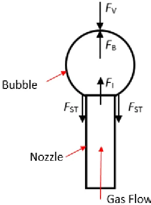
bubble, which are depicted in Figure 1.5. At small gas flowrates, the end of the expansion

phase occurs when the buoyancy (FB) of the bubble in the liquid becomes greater than the

force of surface tension (FST) holding the bubble to the nozzle. As the gas flowrate

increases, the inertia of the gas flow adds an upward force (FI) on the bubble. The

increased flowrate also increases the rate of expansion of the bubble, which in turn,

causes a downward force due to the viscous drag (FV) from the liquid resisting the

(25)

Figure 1.5: Force balance of a bubble in stagnant liquid during the expansion phase. For a low gas flowrate, the Viscous Drag force (Fv) and Gas Intertia Force (FI)

would be negligible.

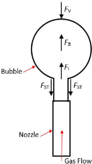
During the detachment stage, the upward forces, mainly the buoyancy, is greater than the

viscous drag resisting the bubble’s upward movement and the surface tension that holds

the bubble to the nozzle. This causes the bubble to accelerate upwards. As the bubble

accelerates upwards, a thin column of gas keeps the bubble in contact with the nozzle and

allows it to continue expanding. Detachment occurs when the buoyancy force becomes

greater than the force of the surface tension of the gas column. As the surface tension

force decreases with increasing local radius, the surface tension of the gas column

decreases as the bubble travels further from the nozzle tip. Once the buoyancy and gas

inertia overcomes the surface tension, the gas column breaks in the middle, closing out

the spherical bubble at the bottom, and allowing a new bubble formation to begin at the

nozzle [26]. Similar to the expansion phase, the upward movement of the expanding

bubble is resisted by the viscous drag of liquid. The force balance for the detachment

(26)

Figure 1.6: Force balance of a bubble in stagnant liquid during the detachment phase.

For tubular absorbers, the upward co-flowing liquid exerts additional drag force on the

bubble causing an early bubble detachment that results in smaller bubble size when

compared to bubble formation in stagnant liquid. A study by Sada et al. [27] identified

the upward forces aiding bubble detachment. Like bubble formation in stagnant liquid,

the gas inertia and bubble buoyancy result in an upward force that opposes the surface

tension holding the bubble to the nozzle. Since the upward flowing liquid must move

around the spherical bubble, the liquid exerts a drag force (FD) on the bubble in the

upward direction. This increases the magnitude of the net the upward force opposing the

surface tension, resulting in smaller bubbles due to early detachment. The force balance

for a bubble in the expansion and detachment phase in upward co-flowing liquid is shown

(27)

Figure 1.7: Force balance of a bubble during the expansion phase (left) and the detachment phase (right) in an upward flowing liquid.

Ramarkrishin et al. [26] discussed the effects of surface tension on the bubble size at

detachment. At low gas flowrates in stagnant fluid, the surface tension and buoyancy

equally contribute to the bubble detachment. As the surface tension of the bubble

increases, the bubble size at detachment increases. As the flowrate increases, the

influence of surface tension on the detached bubble size decreases. Sada et al. [27] also

discussed the effect of surface tension on bubble formation in co-flowing liquid. Due to

the addition of the upward drag force from the co-flowing liquid, the influence of surface

tension decreases further. For inertia (from both the gas and liquid phases) dominated

two-phase flow, surface tension has a negligible effect on bubble size [27].

Another variable that effects the detached bubble size is the nozzle diameter. In the study

by Sada et al. [27] it was observed that a decrease in nozzle size resulted in a decrease in

bubble size at the detachment. If the gas and liquid flowrates remain the same, as the

nozzle diameter decreases, the gas velocity in the nozzle increases, resulting in an

increase in the inertial force of the gas flow acting upwards on the bubble, causing an

F

D

F

D

F

D

F

D

Gas Flow

Liquid Flow

Bubble

(28)

early bubble detachment. For capillary nozzles (diameters <<1mm), it has been shown

that the liquid flow rate has negligible effect on the bubble size [28].

Terasaka et al. [29] reported that the bubble shape at detachment in a liquid co-flow

cannot be spherical. During the expansion stage, the bubble initially has the spherical

shape when it is smaller in size. As it grows, the viscous drag of the co-flowing liquid

stretches the bubble vertical deforming it shape as shown in Figure 1.8. They proposed a

two-dimensional finite element model to predict the bubble shape during formation and

the final bubble volume at detachment. The finite element model considered a balance

between the pressure of the surrounding liquid and the pressure inside of the bubble. It

also considered the force balance between the bubble buoyancy, gas inertia, liquid drag

and surface tension (expressed as the equivalent radii of the gas stem attaching the bubble

to the nozzle) for prediction of detached bubble volume. They compared their predicted

bubble volume from their non-spherical model to the size predicted by spherical bubble

models proposed in previous studies like Sada et al. [27]. It was found that the spherical

bubble models were still able to accurately predict the bubble volume despite not

accurately predicting the bubble shape at the detachment.

Figure 1.8: Bubble shapes during bubble formation from a submerged vertical nozzle in upward flowing liquid as predicted by Terasaka et al. [29].

The model proposed by Terasaka et al. showed the effect of liquid pressure on the bubble

size at detachment [29]. An increase in pressure of the liquid phase generally causes a

(29)

pressure exerts a greater force onto the thin column of gas that attaches the bubble to the

nozzle. This increased force causes the gas column to collapse and detach a smaller

volume bubble when compared to the bubble volume at a decreased pressure. The

pressure effect on bubble size is mainly due to the hydrostatic pressure of the liquid

column. An increase in liquid velocity will decrease the static pressure of the liquid,

however, the increased inertial force will be more than the decrease in the effect of

pressure on the gas column.

1.7 Two-Phase Flow Regimes

The gas flow into a wall-bounded liquid stream could establish a specific structure of the

two-phase flow that depends on the gas and liquid flow rates (GLR). At low gas flow

rates, the gas injected into the liquid forms individual bubbles that are dispersed into the

liquid stream and each bubble remained surrounded by the liquid phase. This flow regime

is called the bubbly flow. As the gas flow rate increases, the bubbles begin to form and

detach more frequently. Eventually the frequency becomes great enough that the bubbles

begin to coalesce after they detach from the nozzle. If the gas flowrate is increased

further, the expansion of the bubble at the nozzle will be fast enough that it coalesces

with the previously detached bubble while still connected to the nozzle. This leads to

flow regimes that can no longer be classified as bubbly flow as there is no clear

separation between bubbles. Through observation of two-phase vertical pipe flow using

x-ray and flash photography, Hewitt and Roberts [30] identified five different flow

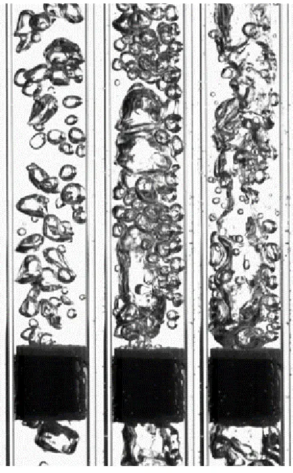
regimes namely, Bubble, Slug, Churn, Annular and Wispy (see Figure 1.9). Bubble, or

bubbly flow is defined as dispersed spherical gas bubbles evenly dispersed in the liquid

phase. As the gas flowrate increases, the bubbles begin to coalesce to form the plug or

slug bubbles present in the slug flow regime. Slug bubbles expand to the pipe wall

causing an intermittent flow of regions of gas and liquid. Slug flow then transitions to

Churn flow as the slug bubbles begin to coalesce and there are limited liquid breaks

between gas phases. Eventually, the gas to liquid flow ratio becomes high enough that the

gas flow becomes the dominant flow in Annular and Wispy flow where the gas

predominantly occupies the core of the tube and the liquid flow is pushed along the tube

(30)

Figure 1.9: Two-phase vertical flow regimes proposed by Hewitt and Roberts [30].

Through observations of the flow regimes at different flow conditions, Hewitt and

Roberts [30] also proposed a flow regime map for the two-phase flow in vertical tubes

(see Figure 1.10). This map can be used to predict the flow regime present in a vertical

(31)

Figure 1.10: Flow regime map for vertical tubular two-phase cocurrent flow proposed by Hewitt and Roberts [30]. The subscripts l and v represent liquid and

gas respectively.

A bubbly flow regime is most desirable for a vertical tubular absorber as it has the

highest surface area to volume ratio. More surface area of the gas phase will allow for

higher mass transfer rates from the gas phase to the liquid phase. Flow regimes such as

slug or churn flow is undesirable as the surface area to volume ratio of the gas phase is

decreased, reducing the mass transfer rate when compared to a bubbly flow. Vertical

tubular absorbers for use in small scale heat absorption refrigeration systems, the required

gas and liquid flowrates are expected to produce slug or churn flow in a conventional

single nozzle system [24, 25], which affects the mass transfer rate. Hence, it is desirable

that the flow regime in the absorber should be bubbly flow to allow for the maximum

(32)

1.8 Motivation

The need for more efficient air conditioning systems has motivated the current research.

Increasing demand for air conditioning will increase global energy demand, resulting in

potential blackouts as energy production struggles to accommodate peak demands. It can

also accelerate the effects of global warming, causing exponential growth as more energy

produced by greenhouse gas emitting sources is needed to provide thermal comfort in

homes throughout the world. The development of a more efficient air conditioning

system, which reduces energy demand from non-renewable resources, is needed. The

heat absorption refrigeration cycle has the potential to greatly reduce energy demand for

residential air conditioning if solar thermal energy is used as its driving energy source.

Studies have been done to test the feasibility of implementing a small-scale heat

absorption refrigeration as a residential air conditioning system and found that the

absorber unit limited the systems performance and design. The performance and size of

the absorber unit is limited by its need for high rates of mass and heat transfer in a

two-phase flow. The present study has been done to improve the understanding of two-two-phase

gas-liquid flow behaviour in vertical circular pipes and to investigate means to improve

the efficiency of a vertical tubular absorber. The investigation focuses on the use of

passive devices to improve the heat and mass transfer rates in the vertical tubular

absorbers. Use of mesh-type bubble breakers in vertical two-phase cocurrent flow has

been shown to be able to reduce the size of a bubble produced by a single gas nozzle in a

two-phase vertical cocurrent flow, thus being a means to increase the mass transfer rate

of a two-phase flow [31]. The previous study on mesh-type bubble breakers [31] is

limited to low liquid and gas flowrates and only covers the bubble breaker’s effect on the

bubbly flow regime. The study also neglects the bubble breaker’s effect on heat transfer,

an important design variable of vertical tubular absorbers. The current study expands on

the previous bubble breaker investigation to investigate the bubble breaker’s effect on a

larger range of two-phase flow regimes, the effect of varying bubble breaker geometry on

flow behaviour, and the effect of mesh-types bubble breakers on heat transfer in

(33)

1.9 Objectives

The specific objectives of this research work are to investigate the effect of various bubble

breaker parameters in vertical two-phase cocurrent flow, on,



The bubble size distribution



The transitional behaviour of various two-phase flow regimes



The two-phase convective heat transfer coefficient

1.10 Research Impact

The results of the current investigation can be used in the development of compact

vertical tubular absorbers for use in small-scale heat absorption refrigeration systems. By

investigating the effect of mesh-type bubble breakers on two-phase flow behaviour,

estimations of their effect on the mass transfer rate in a vertical tubular absorber can be

made. The study on the bubble breaker’s effect on heat transfer in two-phase flow can be

used to make estimates on the heat transfer rate of a vertical tubular absorber. By varying

the geometry of the bubble breakers in both the flow characterization study and the heat

transfer study, the results can be used to optimize the bubble breaker design to maximize

the enhancement of heat and mass transfer rates.

1.11 Thesis Outline

The first chapter is intended to provide a broader overview of the problem of increasing

energy demand for air conditioning and the challenges of implementing solar thermal

heat absorption refrigeration systems as residential air conditioning units. In many studies

that review the feasibility of small-scale solar thermal heat absorption refrigeration

systems, the absorber unit is shown to limit the system performance. The main cause of

the limitation is the reduced mass transfer rates between a gas and liquid phase. It has

been proposed that mesh-type bubble breakers can be used to increase the surface area to

volume ratio of the gas-liquid interface in a vertical tubular absorber to increase the mass

(34)

The second chapter focuses on the investigation of the effect of various parameters of

mesh-type bubble breakers on the bubble size and two-phase flow regime transitions.

The parameters considered in this investigation are the pore size, length and position of

the bubble breaker. A wide range of gas and liquid flow rates were considered that

covered the two-phase flow regimes from bubbly to churn.

The third chapter investigated the effect of mesh-type bubble breakers on heat transfer in

two-phase vertical pipe flow. The results of the effectiveness of mesh-type bubble

breakers as heat transfer enhancement devices are presented and discussed. The effect of

flow regimes on two-phase convective heat transfer is also discussed.

The fourth chapter summarizes the objectives and scope of the present work along with

the key findings from this research. Some future recommendations are also provided to

extend this work and address some unanswered questions from this research.

1.12 Co-Authorship Statement

This thesis has been written in an integrated article format. The second chapter, titled

“Bubble Size Prediction and Flow Regime Analysis for Two-Phase Vertical Co-flow in

the Presence of a Mesh-Type Bubble Breaker” has been submitted to the International

Journal of Multiphase Flow as a separate paper and is co-authored by Kamran Siddiqui.

The third chapter, titled “Two-Phase Vertical Co-Flow in the presence of a Mesh-Type Bubble Breaker” is also co-authored by Kamran Siddiqui and will be submitted to an

(35)

1.13 References

[1] "Energy Efficiency Trends in Canada, 1990 to 2009." Natural Resources Canada.

September 7, 2012. Accessed April 19, 2016.

http://oee.rncan.gc.ca/publications/statistics/trends11/chapter3.cfm?attr=0.

[2] “Air Conditioning in nearly 100 million U.S. homes.” U.S. Energy Information

Administration. August 19, 2011. Accessed April 19, 2016.

https://www.eia.gov/consumption/residential/reports/2009/air-conditioning.cfm.

[3] Auffhammer, M. 2014, “Cooling China: The Weather Dependence of Air Conditioner Adoption.” Frontiers of Economics in China, 9(1), pp. 70-84.

[4] Davis, Lucas. "Air Conditioning and Global Energy Demand." Energy Institute at

Haas. April 27, 2015. Accessed April 19, 2016.

https://energyathaas.wordpress.com/2015/04/27/air-conditioning-and-global-energy-demand/.

[5] Hydro One Networks, Ontario Energy Board, 2003, “Electricity Demand in Ontario.”

[6] "Electricity Prices." Ontario Energy Board. Accessed April 19, 2016.

http://www.ontarioenergyboard.ca/oeb/Consumers/Electricity/ElectricityPrices.

[7] Pidd, Helen. "India Blackouts Leave 700 Million without Power." The Gaurdian.

July 31, 2012. Accessed April 19, 2016.

http://www.theguardian.com/world/2012/jul/31/india-blackout-electricity-power-cuts.

[8] Petri, Y. and Calderia, K. 2015, “Impacts of global warming on residential

heating and cooling degree-days in the United States.” Scientific Reports, 5, pp.

12427-12441.

[9] Sivak, M. 2013, “Will AC Put a Chill on Global Energy Supply?” American

Scientist, 101(5), pp. 101-104.

[10] “Air Conditioning.” Energy.Gov, Accessed April 19, 2016.

http://energy.gov/energysaver/air-conditioning.

[11] “Electricity Data.” U.S. Energy Information Administration, Accessed April 19,

2016.

(36)

[12] Isaac, M. and Van Vurren, D.P., 2009, “Modeling global residential sector energy demand for heating and air conditioning in the context of climate change.” Energy

Policy, 37(2), pp. 507-521.

[13] Biwole, P.H., Woloszyn, M. and Pompeo, C., 2008, “Heat transfers in a double-skin roof ventilated by natural convection in summer time.” Energy and

Buildings, 40, pp. 1487-1497.

[14] Aydin, O., 2006, “Conjugate heat transfer analysis of double pane windows.”

Building and Environment, 41, pp. 109-116.

[15] Kuhns, M., “Planting Trees For Energy Conservation: The Right Tree in the Right Place.” Forestry: Utah State University, Accessed April 19, 2016.

http://forestry.usu.edu/htm/city-and-town/tree-selection/planting-trees-for-energy-conservation-the-right-tree-in-the-right-place.

[16] “Air Conditioning Your Home.” Natural Resources Canada, Accessed April 19,

2016.

http://www.nrcan.gc.ca/energy/publications/efficiency/residential/air-conditioning/6051.

[17] Moran, M. J., and Shapiro, H.N., 2007, Fundamentals of Engineering

Thermodynamics, Hoboken, NJ: John Wiley.

[18] Kalinowski, P., Hwang, Y., Radermacher, R., Al Hashimi, S, and Rogers, P., 2009, “Application of waste heat powered absorption refrigeration system to the LNG recovery process.” International Journal of Refrigeration, 32, pp. 687-694 [19] Nkwetta, D.N., and Sandercock, J., 2016, “A state-of-the-art review of solar

air-conditioning systems.” Renewable and Sustainable Energy Reviews, 60, pp. 1351-1366.

[20] Aman, J., Ting, D.S., and Henshaw, P., 2014, “Residential solar air conditioning:

Energy and exergy analyses of an ammonia-water absorption cooling system.”

Applied Thermal Engineering, 62, pp. 424-432.

[21] Ozgoren, M., Bilgili, M. and Babayigit, O., 2012, “Hourly performance prediction

of ammonia–water solar absorption refrigeration.” Applied Thermal Engineering,

40, pp. 80-90.

(37)

Absorption Chiller for Solar Cooling Applications.” Energy Procedia, 30, pp. 35-43.

[23] Castro, J., Oliet, C., Rodiriguez, I., and Olivia, A., 2009, “Comparison of the

performance of falling film and bubble absorbers for air-cooled absorption

systems.” International Journal of Thermal Sciences, 48, pp. 1355-1366. [24] Fernandez, J., Uhia, F.J., and Sieres, J., 2007, “Analysis of an air cooled

ammonia–water vertical tubular absorber.” International Journal of Thermal

Sciences, 46, pp. 93-103.

[25] Fernandez, J., Sieres, J., Rodriguez, C., and Vazquez, M., 2005, “Ammonia–water absorption in vertical tubular absorbers.” International Journal of Thermal

Sciences, 44, pp. 277-288.

[26] Remakrishnan, S., Kumar, R., and Kuloor, N.R., 1969, “Bubble formation under constant flow conditions.” Chemical Engineering Science, 24 pp. 731-747. [27] Sada, E., Yasunishi, A., Katoh, S., and Nishioka, M. 1978, “Bubble formation in

flowing liquid.” The Canadian Journal of Chemical Engineering, 56, pp.

669-672.

[28] Chuang, S.C., and Goldschmidt, V.W., 1970 “Bubble Formation Due to a

Submerged Capillary Tube in Quiescent and Coflowing Streams.” Journal of

Basic Engineering, 92(4), pp. 705-711.

[29] Terasaka, K., Tsuge, H., and Matsue, H. 1999, “Bubble formation in cocurrently upward flowing liquid.” The Canadian Journal of Chemical Engineering, 77, pp. 458-464.

[30] Hewitt, G.F, and Roberts, D.N. 1969, “Studies of two-phase flow patterns by

simultaneous x-ray and flash photography.” (AERE-M--2159), Technical report,

Atomic Energy Research Establishment, Harwell (England)

[31] Gadallah, A.H. and Siddiqui, K., 2015, “Bubble breakup in co-current upward flowing liquid using honeycomb monolith breaker.” Chemical Engineering

(38)

Chapter 2

2

Bubble Size Prediction and Flow Regime Analysis for

Two-Phase Vertical Co-flow in the Presence of a

Mesh-Type Bubble Breaker

2.1 Introduction

Bubble column reactors are essential components in many chemical and mechanical

processes involving two-phase flows in which the mixing of gas and liquid phases is

required [1-3]. They are widely used due to their capability to allow high rates of heat

and mass exchange between gas and liquid phases. The basic structure of a bubble

column reactor is a vertical cylinder containing flowing or stationary liquid with gas

injected at the bottom of the vessel in the form of bubbles that rise and mix with the

liquid phase and facilitate the heat and/or mass exchange. In the biochemical industry,

bubble column reactors are used as bioreactors for the production of proteins, enzymes

and antibiotics as well as other industrial products [7-12]. Other chemical processes such

as wastewater treatment also utilize bubble column reactors [13-14]. For mechanical

applications, bubble column reactors are used as absorbers units for heat absorption

refrigeration systems [15-17].

In bubble column reactors, the size of the bubble entering the liquid domain is an

important design parameter, since it has a direct influence on the two-phase exchange

process. A large single bubble will have relatively small surface area to volume ratio

compared to numerous small bubbles with the same cumulative volume as the large

bubble. The smaller surface area to volume ratio reduces the interfacial area between the

two phases, which results in the lower heat and mass exchange rates between the two

phases. The growth and detachment of bubbles formed in a two-phase gas liquid vertical

cocurrent flow from a conventional single vertical gas nozzle has been well documented

in the scientific literature. Sada et al. [18] performed an experimental study to measure

the size of single and coalesced bubbles that detached from a single nozzle in an

unbounded vertical liquid flow. Their results show that the bubble size for liquid-inertia

(39)

gas inertial forces, bubble buoyancy forces and the liquid drag on the generated bubble,

to the bubble size and nozzle diameter. They observed that the bubble size increases with

increasing gas flow rate and decreases with increasing liquid flow rate. Teresaka et al.

[19] also investigated the bubble formation in upward flowing liquid in a column.

Through observation of bubble growth at the nozzle tip, they proposed a non-spherical

bubble growth model considering the balance of internal and external pressure forces as

well as the inertial forces from both gas and liquid flows exerted onto the bubble

interface. The model predicted the growth of the bubble volume at the nozzle and the

volume of the bubble after detachment. The bubble size predictions from their model

were in good agreement with experimental results over a range of gas-liquid flow rates

ratio (GLR). However, the model was not able to accurately capture the shape of the

formed bubbles. Chen et al. [20] proposed an interfacial element model to predict the

shape and growth of non-spherical bubbles. They compared the bubble size predicted

from their model with the experimental results from Teresaka et al. [21] and found the

model predictions to be in good agreement with the experimental data. The model also

effectively predicted the shape of a single bubble forming at a nozzle in an upward liquid

flow.

In some applications of bubble column reactors, the ratio of gas-liquid flow rates (GLR)

exceeds the condition at which a single vertical nozzle can produce bubbly flow [15, 16].

Hence, two-phase flow regimes at higher GLRs have been studied in the past. Hewitt [21]

and Hewitt and Roberts [22] studied two-phase flow regimes in both vertical and

horizontal pipes. Through experimental observation of two-phase vertical co-flow, they

identified four regimes: Bubbly, Slug, Churn and Annular. Generally, as the GLR

increases, the flow regime transitions from a bubbly flow to slug, to churn and finally to

annular flow. It has been found that the flow conditions at which the transition from

bubbly to slug flow regime occurs is not very sensitive of the pipe geometry [23]. Flow

transition maps were created to predict the flow regime based on the fluid properties and

flowrates of both phases [21, 22]. However, these maps are valid for the fully developed

(40)

Ujang et al. [24] and Waltrich et al. [25] studied the evolution of two-phase flow from the

entrance region to the fully developed region. These studies show that the flow regime is

not only dependent on the GLR but also that the flow regime changes along the length of

the pipe as the gas regions coalesce. When the gas is injected into the liquid flow, the

initial flow regime may not be the same as the predicted regime from the flow transition

maps proposed by Hewitt, and Hewitt and Roberts [21, 22]. A two-phase flow with gas

and liquid flowrates corresponding with a slug flow regime can begin as a bubbly flow

regime at the pipe entrance immediately downstream of the gas nozzle. As the two-phase

flow continues through the pipe, the initial nozzle generated bubbles begin to coalesce

forming plug and slug bubbles eventually reaching its fully developed flow regime as

predicted by Hewitt [21], and Hewitt and Roberts [22].

For bubble column reactors that operate at high GLRs, the regime is not expected to be of

the bubbly flow, which constitutes the highest surface area to volume ratio for the gas

phase. Hence, to achieve higher mass exchange in the column reactors at high GLRs, a

mechanism needs to be used to break large (slug or churn) gas regions and transition the

regime back to bubbly flow which otherwise would be in slug or churn flow mode.

Several techniques have been reported in literature to generate smaller bubbles or to

break large bubbles. Fadavi et al. [26] investigated the use of a sparger and found a

reduction in the bubble size by adding a rotational flow with a passive swirl device to the

liquid before the gas was released through the sparger. This swirl increased the shearing

force from the rotational liquid and caused early bubble detachment that resulted in

smaller bubble generation. The effect of rotational flow was also investigated by Sobrino

et al. [27]. They used a perforated plate, rotating at a set speed, to release gas into a

fluidized bed. It was found that an increase in the rotational speed of the bed decreased

the bubble size at detachment due to the increase in shearing forces. Manabu et al. [28]

investigated the use of a porous nozzle in a stationary water bath. At low gas flow rates,

the porous nozzle was found to reduce the size of the injected bubbles. As the gas flow

rate increased, the pores’ effectiveness reduced and the gas region similar to the slug

regime was formed in the pipe. They concluded that the pore has no effect at the higher

(41)

The generation of turbulent liquid flow is a common way to control bubble and droplet

size in two-phase flows. The study of turbulence in two-phase flow is dated back to the

pioneering work of Kolmogorov and Hinze [29, 30]. Their studies showed that the size of

a stable liquid droplet in a turbulent liquid flow is dependent on the integral length scale

of the turbulent flow and the turbulent intensity. They proposed a critical Weber number

to predict the stable droplet size in a two-phase flow that relates the shear stress of a

turbulent eddie to the surface tension of the dispersed phase. If the Weber number of a

flow is greater than the critical Weber number, the turbulent shear stress would cause the

droplet to split until the stable droplet size has reached. The same relation can be used in

gas-liquid flows to predict the stable bubble size when the liquid flow is turbulent. In

recent years, studies have been performed to estimate the critical Weber number and

stable bubble or droplet size for a range of specific flows including gas-liquid flow in

tubes [31-34]. By increasing the turbulent intensity in a gas-liquid flow, the chance and

frequency of bubble break-up can be increased allowing smaller and more dispersed

bubbles to be generated.

Passive devices placed downstream of a single nozzle or bubble dispersion system have

also been studied as mechanisms to break up bubbles into smaller daughter bubbles.

These devices can be used to add a shearing force to the flow similar to that of a turbulent

eddie. Miyahara et al. [35, 36] investigated bubble breakup in a two-phase vertical

co-flow by using an orifice plate and a converging-diverging nozzle. Bubbles were formed

from a single nozzle in an upward flowing liquid. The two-phase flow continued through

an orifice plate or converging-diverging nozzle forcing a turbulent jet to form. The

increased turbulence broke the initial bubble into multiple smaller daughter bubbles. A

critical Weber number correlation was developed as a function of the Reynolds number

of the flow through the orifice [36]. The use of multiple sieve trays has been shown to

increase mixing of liquid and gas phases for a variety of flow regimes [37-39]. The

positioning of the trays, the pore size and the opening ratio of the sieves can affect the

bubble size distribution, liquid mixing and gas holdup in a vertical tube. Wire meshes

were studied by Prasser et al. [40] and were found to significantly reduce the size of a

The Effect Of Mesh-Type Bubble Breakers On Two-Phase Vertical Co-Flow

Scholarship@Western

Scholarship@Western

The Effect Of Mesh-Type Bubble Breakers On Two-Phase Vertical

The Effect Of Mesh-Type Bubble Breakers On Two-Phase Vertical

Co-Flow

Co-Flow

Abstract

Keywords

Acknowledgments

Table of Contents

List of Tables

Chapter 3

List of Figures

Chapter 1

Chapter 2

Chapter 3

Chapter 1

1

Introduction

1.1

Global Demand for Air Conditioning

1.2

Vapor Compression Refrigeration

1.3

Heat Absorption Refrigeration

1.4

Challenges with the small-scale implementation of heat

absorption cycle

1.5

Absorber Improvements

1.6

Bubble Formation Process

F

F

F

F

Gas Flow

Liquid Flow

Bubble

1.7

Two-Phase Flow Regimes

1.8

Motivation

1.9

Objectives







1.10 Research Impact

1.11 Thesis Outline

1.12 Co-Authorship Statement

1.13 References

Chapter 2

2

Bubble Size Prediction and Flow Regime Analysis for

Two-Phase Vertical Co-flow in the Presence of a

Mesh-Type Bubble Breaker

2.1

Introduction