Scholarship@Western
Scholarship@Western
Electronic Thesis and Dissertation Repository
11-15-2016 12:00 AM
Evaluation System for Craniosynostosis Surgeries with Computer
Evaluation System for Craniosynostosis Surgeries with Computer
Simulation and Statistical Modelling
Simulation and Statistical Modelling
Jing Jin
The University of Western Ontario
Supervisor Roy Eagleson
The University of Western Ontario
Graduate Program in Biomedical Engineering
A thesis submitted in partial fulfillment of the requirements for the degree in Doctor of Philosophy
© Jing Jin 2016
Follow this and additional works at: https://ir.lib.uwo.ca/etd
Part of the Other Biomedical Engineering and Bioengineering Commons
Recommended Citation Recommended Citation
Jin, Jing, "Evaluation System for Craniosynostosis Surgeries with Computer Simulation and Statistical Modelling" (2016). Electronic Thesis and Dissertation Repository. 4248.
https://ir.lib.uwo.ca/etd/4248
This Dissertation/Thesis is brought to you for free and open access by Scholarship@Western. It has been accepted for inclusion in Electronic Thesis and Dissertation Repository by an authorized administrator of
Craniosynostosis is a pathology in infants when one or more sutures prematurely closes,
leading to abnormal skull shape. It has been classified according to the specific suture that
has been closed, each of which has a typical skull shape. Surgery is the common treatment to
correct the deformed skull shape and to reduce the excessive intracranial pressure. Since
every case is unique, cranial facial teams have difficulty selecting an optimum solution for
each specific patient from multiple options. In addition, there is no standard quantified
measurement to help cranial facial teams to evaluate their surgeries.
We aimed to develop a head model of a craniosynostosis patient which allows neurosurgeons
to practice any potential surgeries so as to simulate postoperative head development. Our
model allows neurosurgeons to foresee the potential surgical results and select the optimal
approach. In this thesis, we have developed a normal head model, and built mathematical
models for possible dynamic growth. We also modified this model by closing one or two
sutures to simulate common types of craniosynostosis. The abnormal simulation results
showed a qualitative match with real cases and the normal simulation indicated a higher
growth rate of the cranial index than clinical data. We believe that this discrepancy was
caused by the rigidity of our skull plates, which will be adapted to deformable skull models
in the future.
In order to help neurosurgeons better evaluate any surgery, we hope to develop an algorithm
to quantify the level of deformity of a skull. We have designed a set work flow and targeted
curvatures as the primary variable. A training data was carefully selected to search for an
ii
validate our algorithm to assess the performance of the optimal system. With a stable
assessment system, we can evaluate a surgery by comparing the preoperative and
postoperative skull shapes of a patient. A surgery can be considered effective when the
postoperative skull has shifted toward a normal shape.
Keywords
Craniosynostosis, computer simulation, virtual reality, skull development, skull shape
iii
Acknowledgments
I would first and foremost like to thank my supervisors Prof. Roy Eagleson and Dr. Sandrine
de Ribaupierre. During my Ph. D and master, they have always provided constructive and
invaluable ideas to lead me progress in my research. I would also like to acknowledge them
for dedicating their valuable time for having weekly meetings, always providing positive
feedbacks to any of my work so as to encourage me toward progressing my thesis. In
addition, I would be appreciated that they provide me a good study atmosphere with a well
equipped office and nice group mates (Arezoo Tony, Trinette Wright and Ryan Armstrong),
from which we are able to help and learn from each other.
I would also like to thank John Lloyd from University of British Columbia for his great
support in providing information and technical help on the simulation software Artisynth
they have developed. It is very generous to share their valuable research experience and let us
to use their updated research outcome.
At the end, I would like to thank to Jonason Lau, who contributed his time on collecting CT
scans of their craniosynostosis patients for me. These are valuable data for me to support me
iv
Table of Contents
Abstract ... i
Acknowledgments... iii
Table of Figures ... viii
Table of Equations ... xviii
Chapter 1 ... 1
1 Introduction ... 1
1.1 Overview ... 1
1.2 Normal Head Development ... 2
1.2.1 The Anatomy of Skull ... 2
1.2.2 Development of Cranial Bones ... 5
1.2.3 Cranial Sutures and Closure... 9
1.3 Craniosynostosis: The Abnormality of Skull Development ... 12
1.3.1 Overview ... 12
1.3.2 Types of Craniosynostosis ... 13
1.3.3 Current Treatment Methods ... 16
1.4 Medical Imaging ... 18
1.4.1 Overview ... 18
1.4.2 Radiography ... 18
1.4.3 Computer Tomography (CT) ... 19
1.4.4 Digital Imaging and Communication in Medicine (DICOM) ... 19
1.5 Previous Work... 20
1.5.1 Overview ... 20
1.5.2 Surgical Evaluation Tool for Craniosynostosis ... 20
v
1.5.4 Automated Diagnosis of the Types of Craniosynostosis ... 22
1.5.5 Statistical Model to Predict Craniosynostosis by the Snake Algorithm ... 23
1.6 Thesis Rationale ... 24
1.6.1 Motivation ... 24
1.6.2 Hypothesis and Objectives ... 25
1.6.3 Outline... 27
Chapter 2 ... 29
2 Head Development Simulation with Pressure Based Hybrid Model ... 29
2.1 Overview ... 29
2.2 Framework of Our Simulation System ... 29
2.3 Simulation Software: Artisynth ... 32
2.4 The Generation of a Head Model ... 33
2.5 Mechanical Properties Setup... 42
2.6 Dynamic Simulation for Each Object ... 45
2.6.1 Brain Expansion ... 45
2.6.2 Suture Stretch ... 47
2.6.3 Skull Extension ... 49
2.7 Set Land Markers On the Skull ... 60
2.8 Results ... 61
2.8.1 Simulations with Only Brain Expansion... 61
2.8.2 Simulations with Skull Plates Extension Added ... 66
2.8.3 Results Discussion ... 76
Chapter 3 ... 77
3 Head Development Simulation with Force Based Model ... 77
vi
3.1.1 Algorithm Specification ... 77
3.1.2 Parameter Specifications ... 78
3.2 Results ... 80
3.2.1 Anterior Plagiocephaly ... 80
3.2.2 Normal Head Development ... 86
3.2.3 Scaphocephaly ... 90
3.2.4 Trigonocephaly ... 94
3.3 Discussions ... 97
3.4 Conclusions and Future work ... 102
Chapter 4 ... 104
4 Evaluation Tool for Craniosynostosis Surgery ... 104
4.1 Overview ... 104
4.2 Curvatures in Differential Geometry ... 105
4.2.1 Curves and Surfaces ... 106
4.2.2 The First Fundamental Form... 108
4.2.3 The Second Fundamental Form ... 109
4.2.4 Normal curvature ... 110
4.2.5 Principal curvatures... 112
4.2.6 Gauss Map and Weingarten Map ... 116
4.3 Estimation of Curvatures for Discrete Surface ... 120
4.3.1 Curvature Estimation Review ... 121
4.3.2 Gauss Bonnet Scheme... 125
4.3.3 Algorithm of Curvature Estimation ... 126
4.4 Skull Shape Evaluation Tool utilizing Statistical Modeling ... 130
vii
4.4.2 Skull segmentation and surface generation... 133
4.4.3 Intracranial Volume Normalization ... 135
4.4.4 Curvature Distribution for One Skull Shape ... 137
4.4.5 Statistical Modeling ... 139
4.5 Results of Evaluating System ... 141
4.5.1 System Optimization ... 142
4.5.2 Result Discussions ... 158
4.5.3 Surgical Assessments ... 162
4.5.4 Conclusions and Future Work... 169
Chapter 5 ... 172
5 Conclusion... 172
5.1 Overview ... 172
5.2 The Simulation of Head Development... 172
5.3 Skull Shape Measurements ... 174
References ... 177
Appendices ... 185
viii
Table of Figures
Figure 1.1: The left view of the anatomy of an adult skull ... 3
Figure 1.2: The outside appearance of an mature occipital bone... 4
Figure 1.3: Infant skull anatomy from both right and top views ... 7
Figure 1.4: Cartilaginous bone in the cranial base is derived from mesodermal sclerotome in blue and neural crest cells in red ... 9
Figure 1.5: Infant suture and fontanelle distributions ... 10
Figure 1.6: Common types of craniosynostosis. The left top skull was scaphocephaly, the right top skull was trigonocephaly, the left bottom skull was brachycephaly, and the right bottom one was anterior plagiocephaly. ... 15
Figure 2.1: Unit shapes that are alternative to form volumetric mesh ... 30
Figure 2.2: The flow chart of the procedure of our head development simulation... 31
Figure 2.3: A screenshot of the GUI of Artisynth... 33
Figure 2.4: A slice of CT scans for the normal baby, using automatic segmentation method in Amira to label out the skull bone with light blue color. ... 35
ix
Figure 2.6: Surface model of a normal head, generated according to segmentation labels.
Different color indicates different skull plates... 38
Figure 2.7: The volumetric mesh of a simplified and smoothed brain ... 39
Figure 2.8: Skull plates were imported in the Artisynth, with gaps between each two plates.
... 40
Figure 2.9: The suture model was indicated with blue color, manually generated with
hexahedral meshes. ... 41
Figure 2.10: An indication of sutures that secrete cartilaginous bone cells. These types of
suture have higher values of Young’s modulus. ... 42
Figure 2.11: The development of circumferences of babies aged within 36 months, where the
horizontal-axis represent the age with respect to months, and the vertical-axis indicates the
values of circumferences with unit of centimeter (cm)... 46
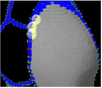
Figure 2.12: Green spheres in this Figure were nodes that were attached onto the closest skull
surface whereas red spheres were not attached to any surface. ... 48
Figure 2.13: This Figure indicates that while the brain volume is expanding, the skull plates
at the suture side are leaving from each, leading to the stretchiness of the suture. ... 49
Figure 2.14: This Figure shows two ways to expand a skull plate. Left one indicates that the
plate was cut at the edge, and make new mesh to fill in, whereas the right one shows to scale
x
Figure 2.15: A skull plate using one sphere to explore the edge. The width of the edge at
the top and bottom is too thick to be accepted. ... 53
Figure 2.16: The skull plate that connected with cranial facial. The red points on the bone
plate indicates this skull edge... 53
Figure 2.17: Illustration of skull edge of right front bone. The red points denote the vertices
we added into the edge list. ... 54
Figure 2.18: An indication of suture stretch. The six blue squares are part of suture, and the
dashed line shows the stretch of the suture. ... 56
Figure 2.19: An indication that changes of the width of a suture could be variant under some
circumstances. ... 56
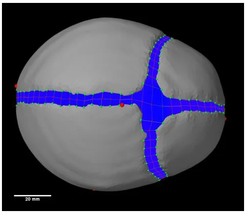
Figure 2.20: The attached suture nodes in green are the centers of each sub-regions. In order
to make this picture clear, we make other plates invisible except this right frontal bone. ... 58
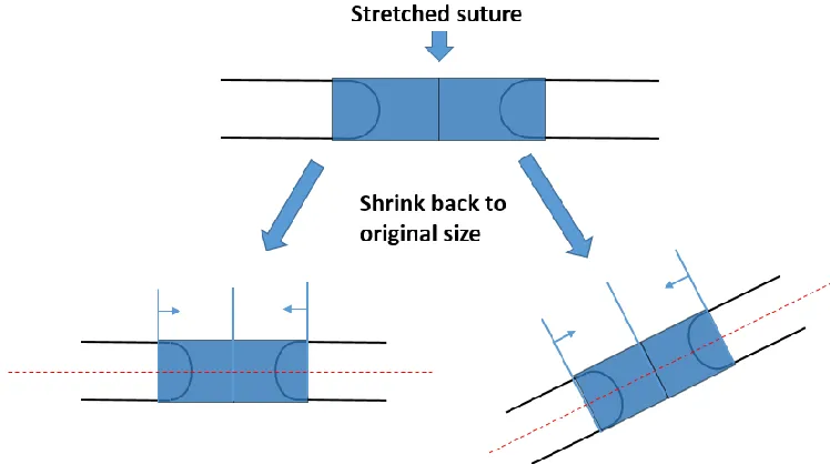
Figure 2.21: The suture shrink back to normal size along the direction of the tension exerted
on it. The blue squares are represented as the cross-sectional view of the suture, where the
shapes outlined with black lines indicated as skull plates. ... 59
Figure 2.22: Six reference markers are set on our normal skull model, to calculate the skull
width, length, and height. The six markers are indicated as red spheres, located at the left,
right, front, back, top and bottom of the skull respectively. ... 61
Figure 2.23: The length, width, height and volume measurement with respect to time during
xi
right Y-axis indicated the volume of the skull with unit of dm3, and x-axis represented time
with seconds. ... 63
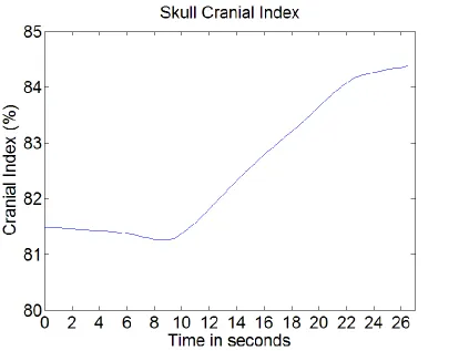
Figure 2.24: The values of cranial index over time during the simulation, which is the
relation between skull width and skull length... 64
Figure 2.25: A screen shot of our head model in the middle of the simulation with color map
of stress showing minimum as no tension to maximum as red... 65
Figure 2.26: A screen shot of our normal head model at the end of the simulation. ... 66
Figure 2.27: Original status of our normal skull model, and the brain model was placed inside
the skull. The red spheres are reference markers. ... 67
Figure 2.28: A deformation of our head model at the end of our simulation, left indicated
from top view, and right displayed from front view. ... 68
Figure 2.29: A screen shot of our normal head model in the end of the simulation, left
showed from left view, and right indicated from back view. ... 68
Figure 2.30: The values of cranial index calculated at each time intervals during the
simulation, where x-axis represented time in seconds, y-axis denoted cranial index... 70
Figure 2.31: The original status of our scaphocephaly model, where the sagittal suture is
closed. ... 71
Figure 2.32: A screenshot of our scaphocephaly at the end of the simulation, showing a long
xii
Figure 2.33: Cranial index values of the simulation of scaphocephaly. ...72
Figure 2.34: Initial status of our trigonocephaly where the frontal suture was closed. ... 74
Figure 2.35: The result of the simulation with closed frontal suture. ... 74
Figure 2.36: Cranial index values during the simulation of trigonocephaly model... 75
Figure 2.37: a) Initial plagiocephaly model. b) Plagiocephaly model in the middle of simulation. ... 76
Figure 3.1: An indication of the relationship between face normal and the force fo'i... 78
Figure 3.2: a) One of the suture that was segmented from original model, crossing the cranial facial bones. b) The other suture we segmented, located at the cranial base. ... 80
Figure 3.3: Initial model of anterior plagiocephaly by closing the right side of coronal suture. ... 81
Figure 3.4: Top view of our plagiocephaly model in the end of the simulation, the opened frontal bone was protruded while the affected side remained original status. ... 82
Figure 3.5: Front view of our initial plagiocephaly model. ... 83
Figure 3.6: Front view of the result from plagiocephaly simulation. ... 84
Figure 3.7: The scales of the skull during the simulation of plagiocephaly head development. ... 85
xiii
Figure 3.9: Top view of our normal head model, left presented the initial status and right
was captured in the middle of the simulation. ... 86
Figure 3.10: Front view of our normal head model, left presented the initial status and right
was captured in the middle of the simulation. ... 87
Figure 3.11: Side view of our normal head model, left presented the initial status and right
was captured in the middle of the simulation. ... 87
Figure 3.12: The scales of the skull during the simulation of normal head development. ... 89
Figure 3.13: Cranial indices with respect to time during the normal head development
simulation. ... 89
Figure 3.14: Top view of our scaphocephaly head model, left presented the initial status and
right was captured in the middle of the simulation. ... 90
Figure 3.15: Front view of our scaphocephaly head model, left presented the initial status and
right was captured in the middle of the simulation. ... 91
Figure 3.16: Side view of our scaphocephaly head model, left presented the initial status and
right was captured in the middle of the simulation. ... 91
Figure 3.17: The scales of the skull during the simulation of scaphocephaly head
development. ... 93
Figure 3.18: Cranial indices with respect to time during the scaphocephaly head development
xiv
Figure 3.19: Top view of our trigonocephaly head model, left presented the initial status
and right was captured in the middle of the simulation. ... 94
Figure 3.20: Front view of our trigonocephaly head model, left presented the initial status and
right was captured in the middle of the simulation. ... 95
Figure 3.21: Side view of our trigonocephaly head model, left presented the initial status and
right was captured in the middle of the simulation. ... 95
Figure 3.22: The scales of the skull during the simulation of scaphocephaly head
development. ... 96
Figure 3.23: Cranial indices with respect to time during the trigonocephaly head development
simulation. ... 97
Figure 3.24: Cranial index statistics from (Likus et al. 2014) ... 98
Figure 3.25: Top view of normal head model during the simulation with deformable skull
plates. ... 101
Figure 3.26: Side view of normal head model during the simulation with deformable skull
plates. ... 101
Figure 4.1: This is the flow chart of our statistical modeling, where 1,2,3 will be adapted
while more input data are involved in the training. ... 132
xv
Figure 4.3: Results from training data, which the number of faces of each surface mesh is
50000... 144
Figure 4.4: Quantified results with the second mesh simplification method, which reduces the number of faces to the limitations. ... 145
Figure 4.5: NRK vs cranial index with different skull shapes, which number of faces were halved four times... 146
Figure 4.6: NRK vs cranial index with different skull shapes, which number of vertices were at the same level. ... 146
Figure 4.7: Skulls without normalization... 147
Figure 4.8: The measurements of skull shapes with bin=0.0005. ... 148
Figure 4.9: The measurements of skull shapes with bin=0.001. ... 149
Figure 4.10: The measurements of skull shapes with bin=0.01. ... 149
Figure 4.11: The measurements of skull shapes with bin=0.004. ... 150
Figure 4.12: The measurements of skull shapes with bin=0.005. ... 151
Figure 4.13: The measurements of skull shapes with bin=0.006. ... 151
Figure 4.14: The measurements of skull shapes with bin=0.008. ... 152
Figure 4.15: The measurements of skull shapes from test data with bin=0.005. ... 153
xvi
Figure 4.17: The quantified results of skull shapes with new data added. ...156
Figure 4.18: Top view of trigonocephaly skulls, the left one is a typical shape and the right
one is an untypical case... 156
Figure 4.19: Side view of trigonocephaly skulls, the left one is a typical shape and the right
one is an untypical case... 157
Figure 4.20: Comparison of skull shapes from top view, the left one is from a brachycephaly
patient and the right one is from plagiocephaly case 1. ... 157
Figure 4.21: Comparison of skull shapes from top view, the left one is from plagiocephaly
case 1 and the right one is plagiocephaly case 2. ... 158
Figure 4.22: An indication of expected areas of shape results for each type of skull shapes.
... 161
Figure 4.23: A comparison of local shapes between two scaphocephaly patients (right is case
1 and left is case 2), indicated by color map of curvature values showing from blue as 0 to
red as higher than 0.1. ... 162
Figure 4.24: Surgical evaluation of a scaphocephaly case with one preoperative and one
postoperative skull shapes... 164
Figure 4.25: Surgical evaluation of another scaphocephaly patient with one preoperative and
one postoperative skull shapes. ... 164
Figure 4.26: Surgical evaluation of a trigonocephaly patient with one preoperative and one
xvii
Figure 4.27: Surgical evaluation of a brachycephaly patient with one preoperative and one
postoperative skull shapes... 166
Figure 4.28: Surgical evaluation of a plagiocephaly patient with one preoperative and one
postoperative skull shapes... 167
Figure 4.29: Surgical evaluation of another plagiocephaly patient with one preoperative and
one postoperative skulls. ... 168
Figure 4.30: Skull shapes with color map of curvature values, showing from blue as 0 to red
as higher than 0.1. The left skull was taken preoperatively and the right one was
postoperative. ... 168
xviii
Table of Equations
Equation 2.1: Brain center calculation. ... 47
Equation 2.2: The position of brain nodes updating equation over time. ... 47
Equation 3.1: The calculation of forces applied on the interior surface of skull. ... 78
Equation 4.1: The expression of a surface by two parameters... 106
Equation 4.2: The definition of a space curve on a surface. ... 107
Equation 4.3: The definition of tangent vector on a surface. ... 107
Equation 4.4: The expression of the tangent surface at a given location of a surface. ... 107
Equation 4.5: The distance calculation between two points on the surface that is infinitely close to each other. ... 108
Equation 4.6: The approximation of the arc length between two close points on the surface. ... 108
Equation 4.7: The first fundamental form... 109
Equation 4.8: The expression of first fundamental form in matrix. ... 109
Equation 4.9: The second fundamental form. ... 110
Equation 4.10: The matrix expression of the second fundamental form. ... 110
xix
Equation 4.12: The definition of curvature. ...111
Equation 4.13: The definition of normal curvature... 111
Equation 4.14: The normal curvature with respect to the fundamental forms... 112
Equation 4.15: An alternative way to express normal curvature. ... 112
Equation 4.16: The normal curvature expression at extreme values. ... 112
Equation 4.17: The relationship between the coefficients at extreme values. ... 113
Equation 4.18: Extended expression of normal curvature at extreme values. ... 113
Equation 4.19: The quadratic equation of normal curvature at extreme values. ... 113
Equation 4.20: Gaussian curvature. ... 114
Equation 4.21: Mean curvature. ... 114
Equation 4.22: Principal curvatures. ... 114
Equation 4.23: Gauss map. ... 116
Equation 4.24: The tangential map derived from the Gauss map. ... 116
Equation 4.25: The definition of Weingarten map. ... 117
Equation 4.26: The projection of tangent vector by Weingarten map. ... 117
Equation 4.27: The second fundamental form represented by Weingarten map. ... 117
xx
Equation 4.29: The relationship between the principal curvatures and any normal curvature
on a given location of a surface. ... 118
Equation 4.30: The definition of the shape operator... 119
Equation 4.31: The relationship between Gaussian curvature and the shape operator. ... 119
Equation 4.32: The interpretation of Gaussian curvature with respect to Gauss map. ... 120
Equation 4.33: An alternative way to calculate the value of Gaussian curvature. ... 120
Equation 4.34: The estimation of normal for each vertex. ... 127
Equation 4.35: The estimation of normal curvature. ... 128
Equation 4.36: The calculation of the tangent vector associated with a specific normal curvature... 128
Equation 4.37: The expression of normal curvature with a given coordinate system. ... 129
Equation 4.38: The estimation of Gaussian, Mean and Principal curvatures. ... 130
Equation 4.39: The calculation of the centroid of the skull model. ... 136
Equation 4.40: The normal vector of the sagittal plane. ... 136
Equation 4.41: The formula to check whether a vertex in on the sagittal plane. ... 137
Equation 4.42: The definition of mean. ... 140
xxi
Equation 4.44: The equation to calculate skewness. ...140
Equation 4.45: The definition of kurtosis ... 141
Chapter 1
1
Introduction
1.1
Overview
During the first year of human life, an infant’s skull develops from several pieces,
connected with each other by a type of soft tissue, which plays a key role in the
development of the skull. The gap between each of two skull plates is referred to as one
suture. During the first year, sutures are ossified one by one at different times. Each
suture is closed until finally the skull is combined into one piece. The timing of the
closing sutures determines how the skull will be shaped. However, there is a pathology
that occurs in infants wherein one or more sutures are closed prematurely, leading to a
malformed skull shape. Given the importance of appearance and proper neurological
development, surgery is a regular treatment to attempt to correct the skull shape.
In this chapter, we will first introduce how the skull and sutures are formed while in utero
and how they develop in the first year after birth. Next, we will introduce
craniosynostosis, including the types, the causes, and treatments. Studies by other
research groups that try to facilitate neurosurgeons’ performance of surgeries for
craniosynostosis will be discussed. Finally, we will explain the structure of our two
projects intended to improve the surgical treatment of craniosynostosis and how it differs
1.2
Normal Head Development
The skull plates of an infant start to develop while in utero, and the sutures are formed a
few weeks before delivery. Approximately six months after delivery, the sutures start to
close, which begins to secure the skull shape. In this section, we will first briefly
introduce the anatomy of a skull, our primary interest is with the cranium, including its
development from several pieces above the brain. Subsequently, the formation of sutures
will be discussed, as well as the role they play in establishing skull shape during infancy.
1.2.1
The Anatomy of Skull
The human skull is a bony structure supported by the spinal column, and is composed of
two parts, the cranium and the facial skeleton (Clemente 1985; Larsen 2002). In our
research, we are only concerned with the cranium. The cranium of an adult, which
protects the brain, consists of eight skull plates: the occipital, frontal, sphenoidal, and
ethmoidal, left and right parietal, and left and right temporal respectively. All these plates
are joined together by sutures, which are classified as rigid articulations that rarely allow
movements in adults (Ellis and Mahadevan 2010; Hartwig 2008). Figure 1.1 below shows
Figure 1.1: The left view of the anatomy of an adult skull
[https://en.wikipedia.org/wiki/Skull#/media/File:Human_skull_side_bones.svg]
The occipital bone (shown in Figure 1.2), located at the back and inferior part of the
cranium, has a large aperture called the foramen magnum, which translates to big hole,
where the vertebral canal connects to the skull (Larsen 2002). The occipital bone consists
of four parts. With reference to the foramen magnum, the squama portion is a scale
shaped plate above this hole, developed from membrane, while the basilar part is beneath
the hole and the lateral parts are on either side. With the exception of the squama, the
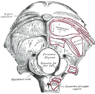
Figure 1.2: The outside appearance of an mature occipital bone
[https://en.wikipedia.org/wiki/Occipital_bone#/media/File:Gray129.png]
The frontal bone is composed of three structures: the forehead, the top of the eye sockets,
and the forepart of the cranial roof. It is separated by the frontal suture into left and right
parts at the very beginning of human life, which is fused after the second month of fetal
development, and disappears by age 6-8 (Tortora and Nielsen 2010).
The two temporal bones constitute the bottom of the cranial sides and part of the cranial
base. Each temporal bone is categorized into five parts according to its anatomical
structure: squama, petrous, mastoid, tympanic, and the styloid process. At the end of fetal
growth, each temporal bone has three major portions: the squama, which is a relative flat
from cartilage in the ear capsule; and the tympanic ring, to which the tympanic
membrane is attached. The styloid process is formed after birth.
The larger part of the cranium sides and roof consist of two parietal plates, each of
which looks like an irregular quadrilateral with four borders and two surfaces (Hartwig
2008). At the center of the cranial cavity is the sphenoid bone, which is called the
"keystone of the cranial floor" because it associates with all the other bones in the
cranium (Tortora and Nielsen 2010). Its shape is similar to a bat with two pairs of
extended wings (greater wings and lesser wings). The ethmoid bone is situated in the
middle of the anterior cranial base and between the two eye sockets, constituting the roof
of the nose (Ellis and Mahadevan 2010). It is an extremely light weight and porous
structure (Clemente 1985).
1.2.2
Development of Cranial Bones
The human cranium is composed of two different bone tissues, which categorize the
cranium into two parts: intramembranous bone is the cranial vault or calvaria (which
includes the roof and sides of the neurocranium and the face) and cartilaginous bone
which is the cranial base (called chondrocranium) (Moss 1954). These two essential
components of bone tissue are created during fetal development (Dye 2000; Steinbock
2011).
The cranium is formed from mesenchymal cells, which first appear as membrane
enclosing the growing brain (Sperber, Sperber, and Guttmann 2010). This membrane
contains two layers: the internal layer, known as the endomeninx, which is derived from
from both the paraxial mesodermal and neural crest cells. The endomeninx gives rise to
two further layers: the pia mater and the arachnoid that cover the brain. The ectomeninx
also forms two distinct layers: the unossified internal dura mater that covers the brain and
an external membrane, which either ossifies into bones at the cranial vault, or condrifies
into cartilage at the cranial base. The structure of the membrane is shown in the following
Figure 1.3. The dura mater that encircles the brain prevents the brain from developing
into a complete sphere, and acts as the endocranial periosteum, which also affects the
shape of the cranial vault. Some researchers have also pointed out that dura mater is
necessary for intramembranous bone formation, by serving a role in ossification
Figure 1.3: Infant skull anatomy from both right and top views
On the external layer of the ectomeninx, several primary and secondary ossification
centers are formed and spread out as individual flat bones (Moore, Persaud, and Torchia
2011). The ectomeninx originates from two different sources, the mesodermal cells
which form major parts of the frontal, parietal, sphenoid, petrous temporal and occipital
bones, and the neural crest cells, which give rise to the squamous, temporal, lacrimal,
nasal, zygomatic bones, etc… (Sperber, Sperber, and Guttmann 2010). Around
right superciliary arch and ossify into the left and right frontal bones. Secondary centers
subsequently arise at each side of the zygomatic processes, nasal spine, and trochlear
fossae, then fuse together with each primary frontal center. Each of the parietal bones
emerge from two primary ossification centers at eight-weeks pc, which fuse together after
two months. The squamous part of the temporal bone develops from solitary centers,
whereas the tympanic ring develops from four. The fusion of these two parts occurs at
birth, while the rest of the temporal bone develops from cartilage. Although most of the
ossification centers arise around the seventh and eighth week pc, the outward extension
of the ossification continues after birth.
At the fourth week pc, mesenchyme aggregates around the notochord that is beneath the
hindbrain, beginning to form the floor of the external layer of ectomeninx. The notochord
is formed during the embryonic stage, and will form the midline axis as well as play a
role inducing the development of surrounding tissues. The sella turcica is a saddle-shaped
region of the sphenoid bone of the human skull and contains the pituitary fossa at its
centre (shown in Figure 1.4). Bones located anterior to this point are formed by neural
crest cells, which labeled in blue in Figure 1.4, whereas bones posterior to it, indicated in
red in Figure 1.4, are formed by the mesodermal sclerotome. The condrocranium also
begins from separated cartilage centers, which occur at certain locations and periods, then
fuse together to form either entire or partial plates of the cranial bones. For example, the
sphenoid, and the ethmoidal bones are entirely formed from cartilage, whereas the only
base of the occipital plate, the petrous and mastoid parts of the temporal plate are formed
Figure 1.4: Cartilaginous bone in the cranial base is derived from mesodermal
sclerotome in blue and neural crest cells in red
[http://skeletalsystemdev.weebly.com/development-of-skull.html]
1.2.3
Cranial Sutures and Closure
Although the ossification of intramembranous bones spreads out after each primary
center appears, these bones become broadly separated because of the faster growth of the
continues. The mesenchyme between the bones is induced by underlying dura mater to
develop fibrous tissues, named sutures, but only when two bone fronts are close enough
to each other. A similar process occurs with the development of fontanelles, though they
consist of an interface of more than two bones (Opperman 2000; Moss 1954).
Figure 1.5: Infant suture and fontanelle distributions
Figure 1.5 above depicts all the sutures and fontanelles that develop during infancy. The
frontal suture, also known as the metopic suture, is between the left and right frontal
bones. This suture starts to close from front to back around the second month pc and
normally disappears between nine months and two years. The sagittal suture is the
the Parietal bones and the Occipital bone. The left and right coronal sutures are between
the left frontal and parietal bones and the right frontal and parietal bones respectively.
Unlike the frontal suture, the fusion of these sutures is from back to front or from side to
center, occurring at different times for each individual.
The anterior fontanelle (closes later from 1 to 3 years) is a soft spot at the front top of the
cranium, converged upon by the frontal, sagittal, and coronal sutures. The Posterior
fontanelle is at the back of the cranium and in the middle of sagittal suture, and closes
after 2-3 months. The squamosal sutures are between the parietal bones and temporal
bones, which, with the coronal sutures, form the sphenoidal fontanelles (closing around 6
months). The mastoid fontanelles (which close between 6 and 18 months) are formed by
the squamosal and lambdoidal sutures (Pritchard, Scott, and Girgis 1956).
Sutures play a significant role as skull bone growth sites while remaining patent for brain
expansion inside (Dye 2000; Steinbock 2011). In other words, in order to accommodate
the expanding brain, sutures produce new bones at the bone fronts, which are attached to
sutures, while maintaining the suture itself at approximately the same size and in an
unossified state but increase the volume of the bones (Opperman 2000). (Opperman
2000) believed that bone growth sites, unlike the bone growth center, are passive bone
remodeling regions without intrinsic growth ability, and need to be triggered by external
stimuli. In cranium development, the key external stimulus is believed to be the enlarging
brain, which exerts pressure on the internal surface of the calvarium to separate the
intramembranous bones and stretch the suture, thereby stimulating the stretched sutures
to develop more bones and go back to their original size (Reardon 2000). Therefore, skull
to maintain their size by adding more bones at the edges of the bone fronts to compensate
for the increasing calvarial volume (Sperber, Sperber, and Guttmann 2010).
Moreover, these flexible and transitory disconnections (sutures) among these cranial
plates are essential to assisting the infant's head as it passes through the birth canal and
meanwhile avoiding brain damage (Steinbock 2011). After birth, the flexibility of the
sutures and fontanelles can also absorb external forces to shield the brain when the
infant's head is slightly knocked (Gilbert and Singer 2006).
1.3
Craniosynostosis: The Abnormality of Skull
Development
1.3.1
Overview
Obviously, the sutures are significant during the early development stage, as otherwise a
pathology called craniosynostosis would take place, when one or more sutures close
prematurely (Johnson and Wilkie 2011). Because the brain is blocked from developing in
the perpendicular direction of the closed sutures, it is forced to over expand in the
perpendicular directions of other opening sutures, resulting in a distorted head shape and
deformed facial features (Johnson and Wilkie 2011). The discovery of craniosynostosis
can be traced to 1851, when (Virchow) first indicated a type of skull abnormality caused
by prematurely closed sutures.
The exact cause of this pathology is still unknown, but may be related to both genes and
(Aviv, Rodger, and Hall 2002). It is a relatively highly frequent pathology in newborns
such that one subject may be found in every 2500 newborns, and so it has received much
attention since some cases of it may contribute to high intracranial pressure and certain
developmental delays (Pritchard, Scott, and Girgis 1956).
1.3.2
Types of Craniosynostosis
Craniosynostosis is categorized into four types depending on which suture is fused:
Trigonocephaly (frontal suture closed), Scaphocephaly (sagittal suture closed),
Plagiocephaly (either of coronal or lambdoid suture closed), and Brachycephaly
(bicoronal suture closed), among which the first two are the most common types. We
have indicated the typical shape of these skulls in Figure 1.6.
Among the most common types of pathological cases, scaphocephaly, the sagittal suture
is fused, causing a long, boat-shaped head. The frequency of scaphocephaly, according to
statistics, is around one in every 5000 children (Pritchard, Scott, and Girgis 1956). The
brain’s development is hindered in the perpendicular direction of the sagittal suture, and
thus expands more in the direction of the sagittal suture to accommodate this blockage.
The temporal brain lobes could be pressed in such conditions, leading to disorders of
hearing, sound perception or pronunciation.
Trigonocephaly occurs when the metopic suture (separates the frontal bones) is fused
before 9 months or even prenatally (normally closed between 9 months to 2 years),
leading to a triangular forehead (Pritchard, Scott, and Girgis 1956). As the second most
common type, the frequency of occurrence is approximately one in every 15,000
problems with vision and ocular hypotelorism. In this situation, it is necessary to rebuild
the whole forehead to regain a regular shape.
Plagiocephaly is further classified into anterior plagiocephaly and posterior
plagiocephaly. Anterior plagiocephaly, whose prevalence is estimated to be 1 in every
10,000 births, is the premature closure of either side of the frontal suture, whereas the
fusion of the unilateral lambdoid suture as known as posterior plagiocephaly (Pritchard,
Scott, and Girgis 1956). The appearance of anterior plagiocephaly could be evidence of
facial deformity in some cases while posterior plagiocephaly creates a flat surface at the
unilateral back of the head. Both types of plagiocephaly could lead to visual impairment
and higher intracranial pressure.
Brachycephaly is treated as premature closure of the bilateral coronal suture, preventing
the brain from growing in the perpendicular direction of the lateral suture so that it
develops more in the closed suture direction. The skull is compressed in the sagittal
direction and extensively in the transverse direction, leading to eyeball protrusion and a
flat head as the most obvious symptoms. In such cases, the intracranial pressure could be
Figure 1.6: Common types of craniosynostosis. The left top skull was scaphocephaly,
the right top skull was trigonocephaly, the left bottom skull was brachycephaly, and
1.3.3
Current Treatment Methods
Surgery is considered the routine treatment for craniosynostosis patients in order to
correct the skull shape and reduce the excessive intracranial pressure caused by suture
fusion. (Lannelongue 1892) performed the first surgery for a craniosynostosis patient.
(Jane et al. 1978) shared their experience adjusting the frontal prominence of a
scaphocephaly patient with the Pi () technique. It is called Pi technique since the shape
of the cuts on the cranial roof looks like “”. Again, (Jane et al. 1984) utilized dural
plication to correct plagiocephaly. (Albright 1984) described parietal wedge
craniectomies for the treatment of scaphocephaly. (Greene and Winston 1986) published
their treatment for scaphocephaly, which included sagittal craniectomy and bi -parietal
morcellation. (Persing et al. 1989) proposed near-total cranial vault reconstruction for the
treatment of brachycephaly. (Cohen et al. 1991) published their treatment for
craniosynostosis using fronto-orbital remodeling with the advancement-onlay technique.
A sunrise technique was published for surgical treatment of occipital plagiocephaly by
(D. F. Jimenez and Barone 1995). This technique focuses on reopening the fused
lambdoid suture and reconstructing the flattened occipital bone (D. F. Jimenez and
Barone 1995).
(Vicari 1994) first applied the endoscopic technique for craniosynostosis treatment.
Endoscopic technique aims to complete a surgery with small incisions and endoscopic
instruments that help view the internal body of a patient (Barone and Jimenez 1999).
(Barone and Jimenez 1999) combined the endoscopic craniectomy with helmet wearing
vault reconstruction utilizing biodegradable plates in minimally invasive craniosynostosis
repair in 2002.
So far, the surgical treatments for craniosynostosis have developed from simple suture
re-opening procedures to cranial vault reconstructions (Thaller, Bradley, and Garri 2007).
Generally, neurosurgeons have believed that the best time for surgical treatment for a
craniosynostosis patient is between two to four months, when the skull bone is relatively
soft and has potential to grow. We will introduce some popular approaches for common
types of craniosynostosis described in (Thaller, Bradley, and Garri 2007).
1.3.3.1
Scaphocephaly
Various approaches are applied for scaphocephaly determined by the severity and the age
of the patient. If the deformity has been diagnosed in early stage, neurosurgeons would
suggest sagittal synostectomy only. The Pi technique could be applied for patients that
only appeared with frontal bossing but no saddling or occipital abnormalities (David F.
Jimenez et al. 2002). To infants that has significant deformity, a cranial vault remodeling
should be preformed with biodegradable plates and screws.
1.3.3.2
Trigonocephaly
(Noetzel et al. 1985) summarized that no matter the severity of the abnormality, the
surgical procedures are quite consistent. The routine approach is osteotomies on bilateral
supraorbital rim, in which a temporal tenon or Z-plasty might be considered with the
extensive interorbital separation for patients with hypotelosrism. Helmets are suggested
to wear postoperatively for several months.
1.3.3.3
Unicoronal and Bicoronal Synostosis
Depending on the level of deformity of this pathology, the surgical procedures are
variant. Normally, supraorbital rims osteotomies and bifrontal craniotomy are
accomplished. For patients with specific facial abnormalities, more osteotomy might be
carried out. Fronto-orbital advancement technique and cranial reconstruction are carried
out for brachycephaly cases.
1.4
Medical Imaging
1.4.1
Overview
Medical imaging is a technique that allows to visualize interior part of a human body or
the functions of some organs, to assist disease diagnosis, monitoring and treatment. It can
be sub-classified into various modalities, including radiography, ultrasound, computer
tomography (CT), magnetic resonance imaging (MRI), nuclear medicine and so on.
1.4.2
Radiography
Radiographic technique was developed firstly from the discovery of x-rays in 1895 by the
physicist Wilhelm Roentgen (Bushberg 2002). The x-rays are emitted from an x-ray tube
above one side of human body, and penetrate through the body to reach the x-ray
detectors on the other side, from where to produce x-ray images. Different tissues in
by (also known as x-ray attenuation), resulting to discrepant amount of x-ray energies
distributed on the detectors, which show different tissues with different intensities.
1.4.3
Computer Tomography (CT)
Computer tomography (CT) is an imaging technique that produces cross-sectional images
using x-ray technique for diagnostic and therapeutic purposes in clinics. While an x-ray
image is an 2D representation of a volume of human part, CT can be interpreted in a way
that taking several 2D x-ray images of the volume from different angles to reconstruct the
anatomy of the whole volume in 3D.
X-ray CT is capable of showing superior contrast between bone and soft tissues, which
make CT scans as a standard diagnosis procedure and surgical planning material for
craniosynostosis patients.
1.4.4
Digital Imaging and Communication in Medicine (DICOM)
Digital Imaging and Communication in Medicine is defined as a standard protocol of
handling, transmitting and storing information in medical imaging. The concept was first
introduced by the American college of Radiology (ACR) and National Electrical
Manufacturers Association (NEMA) in 1983. DICOM covers disciplines of images
compression, visualization, image presentation and so on (Kahn et al. 2007).
Each DICOM file represents a cross-sectional image with a matrix of pixels, each of
which contains a grayscale. With appropriate mathematics, we can extract 3D geometry
existed now to support visualizing and manipulating DICOM images, such as 3D Slicer,
Amira and so on.
1.5
Previous Work
1.5.1
Overview
In previous sections, we have explained the pathological situations that might occur
during skull development for infants and corresponding treatments. Considering the
ethical problem, the studies for infant’s skull growth has been developed very slow.
Recently, with the rise of virtual reality concept and three-dimensional (3D) medical
imaging techniques, some of the research groups start to devote to improving the
treatment for craniosynostosis. In this section, we will discuss most related work (2010 -
2016) with respect to virtual reality and medical imaging techniques.
1.5.2
Surgical Evaluation Tool for Craniosynostosis
In their paper (Oliveira et al. 2010) , Oliveira et al. introduced an evaluation system to
measure the outcomes of craniosynostosis surgeries, utilizing image registration
technique. For their system, three sets of CT scans of a patient are required, which
includes scans of preoperative, postoperative, and one-year postoperative. With the
preoperative images as a reference, the other two images were transformed to align with
the reference. They indicated the local changes (visually and quantitatively) of those two
In the paper, they stated that the minimum distance map is a useful tool to assist
neurosurgeons to evaluate surgery. However, such a tool can only compare the
differences of the skull between before and after surgery, but how do we evaluate a
change as good or not. In our opinion, a good evaluation tool should be able to
investigate the ability of a postoperative skull to grow back to normal shape because of
the surgery.
1.5.3
Finite Element Analysis of Craniosynostosis Adjustment
(Wolański et al. 2013) described an approach to simulate postoperative skull correction
for surgical evaluation, utilizing finite element modeling and analysis. Since the
malformation of each case is variant, it is necessary to design patient specific skull
incisions for each patient (Roth, Raul, and Willinger 2008; Larysz et al. 2011). The
purpose of their work is to choose the best surgical option within various possibilities on
the basis of the quantitative simulation results.
For each patient, (Wolański et al.) used their preoperative computational tomography
(CT) scans to build 3D representation of the deformed skull using finite elements. The
severity of the deformation was quantified in the beginning in order to compare with the
result. For scaphocephaly, the cranial index was measured whereas for trigonocephaly,
the angle of the forehead was measured. With guidance of neurosurgeons, several
surgical options were designed for each patient. In the paper, each case has two possible
solutions. The postoperative skull was then inputted into their simulation software to
examine the ability of the skull to be tilted (bent over). They concluded that the more a
We believed this algorithm has the following limitations. First of all, the simulation of
their surgical correction was based on a condition that all the skull pieces should be
connected as a whole, which is not true for most of real cases. For an infant, we have
discussed in the first chapter, the skull is separated into several plates by sutures since the
brain volume develops faster. Second, the simulation was performed without the
consideration of skull extension itself. During the first year of human life, the skull
development is fast but is varied individually. Therefore, in the middle of skull
correction, the gaps caused by incisions might be closed. Finally, the extent of a skull can
be tilted is not the only factor to assess the surgery for craniosynostosis. For example, for
a scaphocephaly skull that is much longer and narrower than the normal ones, the aim of
the surgery should make the head shorter and wider. However, the tilt capability of a
skull cannot make the skull shorter.
1.5.4
Automated Diagnosis of the Types of Craniosynostosis
(Mendoza et al. 2014) developed an algorithm to quantitatively classify a
craniosynostosis skull and measure the severity of malformation from normal in order to
assist surgical planning for craniosynostosis. Their first step is to generate each patient’s
skull model with normalized orientation and spatial location. With a technique called
graph-cut (Liu et al. 2008), they were able to detect all the open sutures on a skull model,
and to determine if there is a fused suture by comparing to the template (sutures of
normal skull). So far, they can roughly diagnose a skull to be either normal or a type of
craniosynostosis. To further characterize a pathological case from the normal ones, a
normal-skull as a reference. Subsequently, for each skull, local deformation (by
Euclidean distance) and curvature value were calculated to indicate the difference
between this skull and the normal reference.
The authors showed a high-accuracy (95.7%) to auto-diagnose a new skull shape.
However, the abnormity of a skull can be easily deduced by looking at it. In addition, the
shape of each type of craniosynostosis is typical, for example, scaphocephaly patients’
skulls normaly have long-boat shape. Cases that cannot be diagnosed by looking at it can
be treated as not severe cases. In addition, taking CT scans is a standard procedure to
diagnose Craniosynostosis, which makes it much easier to indicate which suture/sutures
are closed. As a result, it cost too much to build a such complex system for diagnosis.
1.5.5
Statistical Model to Predict Craniosynostosis by the Snake
Algorithm
In (Walker et al. 2016)’s work, they measured the asymmetries of intracranial volume
and the patency of each cranial suture to predict the types of craniosynostosis. They used
CT scans of 77 craniosynostosis patients and 40 normal infants to train their predictive
system.
After the skull segmentation on each 2D slide from CT scans of each patient, they used
the snake algorithm to identify the gap (suture) between each two plates, and to refine the
border of the inner surface of the skull so as to measure the intracranial volume
(Hermann et al. 2012). They discovered that the total intracranial volumes of patients
asymmetry of the volume to evaluate the skull shape. Each skull model was divided into
four parts manually with respect to the midlines in horizontal and vertical directions.
Further, they utilized the identified skull bone gaps from CT slides to examine the closure
of sutures. With these two results, they claimed the accuracy of their predictive system
was 91.9%.
As I mentioned in the previous section, the Craniosynostosis can be easily recognized
with CT scans so that a predictive system is not necessary for diagnosis. Moreover, this
system is not completely automatic compared to previous work.
1.6
Thesis Rationale
1.6.1
Motivation
In previous section, we have discussed some common procedures in craniosynostosis that
were introduced in (Thaller, Bradley, and Garri 2007). They also admitted that although
the technique for treatments has been developed, the quantification of surgical evaluation
remained unsolved. Some researchers attempted to use the rate of reoperation to assess
the surgeries (Williams et al. 1997; McCarthy et al. 1995). Alternatively, some
neurosurgeons compared preoperative and postoperative cranial indices (the relation
between maximum skull width and maximum skull length) to measure the surgical
outcomes. However, these two methods failed to describe the changes of local shape.
In addition, without an appropriate assessment method for surgical outcome,
neurosurgeons were not able to validate the efficacy of their surgical techniques. As we
varied. The problem for neurosurgeons then is how to select the most efficient way
among various options. Even for a selected surgical plan, the problem is how far an
osteotomy should be carried out in order to bring the best result. Currently,
neurosurgeons only use their experience to design surgical plans.
In the section of previous work, we have discussed some engineering supports for
craniosynostosis. (Oliveira et al. 2010) developed a tool to measure the difference
between the postoperative skull and preoperative skull, but failed to evaluate the level of
normality for the postoperative skull. (Wolański et al. 2013) described their surgical
simulation system considering only the tilt ability of the skull. (Walker et al. 2016;
Mendoza et al. 2014) used different methods to build an automatic diagnosis system for
craniosynostosis. All of these work did not focus on assisting neurosurgeons in deciding
on how to choose the most appropriate surgical plan for a specific patient and evaluating
how well a surgery has been performed to a patient.
1.6.2
Hypothesis and Objectives
The aim of our research is to develop a predicable model for neurosurgeons to design the
best plan from various options. This model is expected to allow neurosurgeons to carry
out extensive surgical plans on the patient’s head model, and to see corresponding
postoperative skull developments overtime (surgical result).
Computer simulation techniques (van Wijk van Brievingh and Möller 1993), which have
been extensively used in biomedical area currently, allow us to develop such a
predictable tool, without considering ethical issues to perform experiments on infants.
model, including skull, brain and suture. Further, with an appropriate physical modeling,
we can simulate dynamic head development of an infant.
Our hypothesis is that with the ability to simulate a head development, we can accurately
predict surgical result for neurosurgeons by simulating the postoperative skull -brain
growth over time. To address this hypothesis, we have the following objectives:
1) To generate infant’s head models with CT scans and mechanical features, and to
develop mathematical model for dynamic simulation.
2) To simulate both normal and abnormal head development, from which to explore
the mechanism of head development and to validate our simulation algorithm.
3) To perform surgery on patient’s skull model, and simulate postoperative head
development to foresee the surgical result.
In addition, for each skull shape, a NRK is measured, which is capable of describing the
degree of abnormity of a skull with respect to the normal shape. With this tool,
neurosurgeons are able to measure the efficacy of a surgery with the trend of three values,
which includes the shape indices of preoperative and postoperative skull shapes and the
skull shape one-year after the surgery.
Curvature, which describes the local shape of a geometry (Carmo 1976), is able to
characterize different shapes of skulls, in our case, including normal skull and common
types of craniosynostosis. The features will be summarized as a NRK, showing different
values with respect to different shapes. A high value of NRK indicates a high level of
(skull width over skull length), which is an evaluation method for head shape in clinics,
to plot skull shapes onto a 2D Figure for intuitionally visualization.
Our hypothesis then is the NRK for a skull can correctly predict a specific type of skull
shapes, and is able to show the severity of the abnormity of this shape. With this
hypothesis, we have such objectives:
1) To investigate a simple algorithm to estimate curvature values of a skull model,
and to develop a statistical model to calculate NRK.
2) To evaluate a surgery by calculating the shape indices of three skull shapes from
one patient, including skulls of preoperative, postoperative and one-year after
surgery.
1.6.3
Outline
Chapter two contains our initial algorithm (a pressure based model) to simulate infants’
head development during the first year of human life. We used this algorithm to simulate
normal head development, and three common types of craniosynostosis.
Chapter three focuses on introducing our simulation system with a force based model.
We also simulated normal head development and three common types of
craniosynostosis, in order to compare with our previous model.
Chapter four introduces the procedures of developing a statistical model to characterize
deformity of a skull. With this tool, we are able to evaluate the simulation result of any
type of head development, moreover, to evaluate real surgeries.
Chapter 2
2
Head Development Simulation with Pressure Based
Hybrid Model
2.1
Overview
Computer simulation is a technique that uses abstract models to simulate a specific
system on one or more computers (Kheir 1995). It has recently been applied extensively
in biomedical research. This technique can be used to develop surgical simulators, which
help novices to develop their various surgical skills (O’Toole et al. 1999; Duffy et al.
2004; Seixas-Mikelus et al. 2010), to mimic parts of human body (Perktold and
Rappitsch 1995; Stergiopulos, Young, and Rogge 1992; Ghazanfari et al. 2014), and to
test the mechanical properties of specific tissues (Miller et al. 2000). In this chapter, we
attempt to use a computer simulation technique to imitate head development with a
pressure based hybrid model.
2.2
Framework of Our Simulation System
Computer simulation is a technique to simulate the dynamic behaviors of a system on the
basis of a three-dimensional (3D) static model, which in our project is an infant’s head.
Our approach to 3D modeling is mesh generation, also known as grid generation, which
is a technique to describe geometric structures with polygonal or volumetric meshes
(Edelsbrunner 2001). Polygonal meshes delineate the surface of 3D objects with a set of
Volumetric meshes represent the whole volume of 3D objects with finite elements,
including pyramids, tetrahedral, and hexahedral (the shapes are shown in Figure 2.1). The
volumetric mesh is often used to characterize deformable models for finite element
analysis (FEA), which analyze the response to stressby taking account a number of
factors, including mass, volume, temperature, force, and displacement (Krishnamoorthy
1995; Desai 2011).
Figure 2.1: Unit shapes that are alternative to form volumetric mesh
Although the final goal of this project is to simulate postoperative head development, we
hope to first simulate both normal and abnormal head developments, from which it is
easy to validate our algorithm, and to explore how skull shape progresses under different
circumstances. Therefore, we carefully designed a scheme for our initial simulation,
Figure 2.2 below demonstrates our work flow. First, clinical data for an infant head is
acquired in order to label out the structure of the skull. Mesh generation was applied
separately on these segmented structures to develop our 3D head model, which is
essential for our simulation. These assets were then imported into a simulation platform
Artisynth (Fels et al. 2006) and assigned by material properties, such as Young's
modulus, Poisson’s ratio, and the density of each object. Mathematical models were also
built for each structure, to manipulate autonomous behavior or adapt response to extra
stress. Six markers were set on the skull to monitor the maximum length, breadth, and
height of the skull during the simulation.
2.3
Simulation Software: Artisynth
Artisynth, which is a powerful and extensible platform for three-dimensional (3D) object
modeling and simulations, was flexible enough to allow us to implement our hybrid
model (Lloyd, Stavness, and Fels 2012). Artisynth supports numerous types of items,
such as rigid bodies, finite element components, and particles, enabling us to build our
hybrid model. In addition, it is capable of dealing with interactions between any two
components, showing the pressures and forces involved (Vogt et al. 2005), so that we can
interact, display, and ultimately animate a playback of the interactions between a growing
brain and skull. The view point can be changed to let users focus on any part of the
model. Any locations on the model can be marked and traced during the simulation so
that we can produce reports of the evolution of our model across various metrics.
In Figure 2.3, we show a screenshot of the graphical user interface (GUI) of the
Artiysnth. In the main window, we can see the model we have imported, which in this
case is a model of a jaw. On the left side of this main window, is a hierarchy of all the
components involved in the current simulation system. The “Jaw” at the top is the name
of this simulation and the “models” is the document which stores all the objects
associated with this jaw model, including muscle and jaw bone files. Underneath the
main window there is a timeline window, which allows users to track the status of this
model at each time step run in the simulation. After one simulation is done, we can drag
the time back to any frame so that the main window will display the according status of
the model at that particular time. There is a bar of buttons on the left of the documents,
main window, a play button is provided to trigger the calculations for a simulation after
everything has been prepared.
Figure 2.3: A screenshot of the GUI of Artisynth
2.4
The Generation of a Head Model
We have reviewed a set of CT scans from a normal three-week-old baby for our head
provided by the Amira software, which is a platform for 2D or 3D image data
visualization and manipulation. The threshold is selected as 100 Hounsfield Unit (HU),
which means the pixels in the CT slices that have an intensity higher or equal to 100 HU
will be labeled skull tissue. In Figure 2.4, we show one of the slices from the CT images
of this normal baby, where the skull bone has higher intensities then other tissues in the
Figure 2.4: A slice of CT scans for the normal baby, using automatic segmentation
method in Amira to label out the skull bone with light blue color.
The automatic segmentation results are not as we expected. Amira was able to distinguish
the skull from the head very well, but was not able to differentiate between the plates and
the sutures because of the noises produced while taking the CT images and the
narrowness of the sutures. From the Figure 2.4, we can see that there is a disconnection in