FULL PAPER
Probing Earth’s conductivity structure
beneath oceans by scalar geomagnetic data:
autonomous surface vehicle solution
Alexey Kuvshinov
1*, Jürgen Matzka
2, Benny Poedjono
3, Friedemann Samrock
1, Nils Olsen
4and Sudhir Pai
5Abstract
The electric conductivity distribution of the Earth’s crust and upper mantle provides a key to unraveling its structure. Information can be obtained from vector data time series of the natural variations of the magnetic and electric field in a directional stable reference frame. Applying this method, known as magnetotellurics, to oceanic regions is chal-lenging since only vector instruments placed at the sea bottom can provide such data. Here, we discuss a concept of marine induction surveying which is based on sea-surface scalar magnetic field measurements from a modern position-keeping platform. The concept exploits scalar magnetic responses that relate variations of the scalar mag-netic field at the survey sites with variations of the horizontal magmag-netic field at a reference site. A 3-D model study offshore Oahu Island (Hawaii) demonstrates that these responses are sensitive to the conductivity structure beneath the ocean. We conclude that the sensitivity, depending on the bathymetry gradient, is typically largest near the coast offshore. We show that such sea-surface marine induction surveys can be performed with the Wave Glider, an easy-to-deploy, autonomous, energy-harvesting floating platform with position-keeping capability.
Keywords: Marine EM, Wave Glider, Scalar magnetic field variations
© The Author(s) 2016. This article is distributed under the terms of the Creative Commons Attribution 4.0 International License (http://creativecommons.org/licenses/by/4.0/), which permits unrestricted use, distribution, and reproduction in any medium, provided you give appropriate credit to the original author(s) and the source, provide a link to the Creative Commons license, and indicate if changes were made.
Introduction
Magnetotellurics (MT) is an electromagnetic induction method to infer the electric conductivity structure of the subsurface from the measurement of time series of the natural variations of the magnetic and electric field at the surface (Chave and Jones 2012). Knowledge of the con-ductivity structure is of interest for recovering the struc-ture of the Earth’s crust and mantle (Khan and Shankland
2012) and for estimating the influence of induced electric currents in the oceans and mantle on geomagnetic obser-vations on ground and from satellite (Kuvshinov 2008). More and more MT studies are conducted offshore (Baba et al. 2010; Naif et al. 2013; Key et al. 2013) to fill the sub-stantial gap in our knowledge about Earth’s electric con-ductivity structure in the vast oceanic regions. Due to the requirement for a fixed or known sensor orientation
for the vector data, up to now all marine MT studies are based on vector sensors deployed at sea bottom. This is usually logistically as well as instrumentally demand-ing. In this paper, we discuss relatively fast and easy-to-deploy survey concept which is based on sea-surface
measurements of the scalar magnetic field. The method is applicable in the vicinity (a few 100 km) of islands or coasts and can thus address regions of particular tectonic interest like mantle plumes and subduction zones. The underlying idea is to obtain and interpret the responses, i.e., transfer functions, that relate variations of the sca-lar magnetic field at the survey sites with variations of the horizontal magnetic field at a reference site. These “scalar” responses were introduced by Lilley et al. (1984) and independently by Avdeev et al. (1994). In addition, Avdeev et al. (1994) demonstrated that the components of magnetic field can be reconstructed in terms of spa-tial distribution of scalar magnetic field. Later on, Hitch-man et al. (2000) applied the scalar response concept to data obtained from scalar magnetometers floated off-shore on the sea surface. The floating magnetometers
Open Access
*Correspondence: [email protected]
1 Institute of Geophysics, ETH, Zurich, Sonneggstrasse 5, 8092 Zurich, CH,
Switzerland
were deployed in two configurations: one anchored to the seafloor; the second free-floating. Here, we explore an application of the scalar response concept using modern position-keeping platform in the form of an autonomous surface vehicle (ASV) not tethered to the seafloor.
The paper is organized as follows. “Scalar responses” section outlines the derivation of scalar responses. “3-D model study” section presents the results of a 3-D model study which demonstrates the sensitivity of the responses to conductivity structures beneath the ocean. The mod-eled region is Oahu Island (of the Hawaii Islands chain) and surroundings. The Honolulu geomagnetic observa-tory operated by US Geological Survey (USGS) was cho-sen as a reference site. Based on the results of this model study, three suitable offshore sites near Oahu Island were identified and scalar measurements were performed in May–August 2013 using the unmanned, autonomous, wave and solar powered “Wave Glider” ASV. This plat-form was developed and operated by Liquid Robotics Oil and Gas/Schlumberger and was equipped for our field experiment with a towed Overhauser scalar magnetom-eter. “Scalar field measurements using the Wave Glider platform” section provides information about the plat-form, “Data processing” discusses the data processing, and “Observed versus predicted responses” section pre-sents a comparison of the predicted responses with those estimated from the data. “Conclusions and discussion” section contains conclusions and discussion. The paper also includes two appendices in which alternative “scalar” responses are introduced.
Scalar responses
This section sketches the derivation and explanation of scalar responses and closely follows the line of reasoning and nomenclature used by Avdeev et al. (1994).
Deriving the scalar responses one relies on two assumptions: (a) The source of the time-varying magnetic field is a vertically incidenting plane wave; (b) the magni-tude of magnetic field variations, B(r,t), is much smaller than the magnitude of the static ambient (main) mag-netic field, B0(r), i.e.,
The latter assumption allows to represent time variations of the scalar field, F(r,t), in the following form
where p stands for the normalized static main field (or
in other words for the unit vector in the direction of the main field)
Transforming Eq. (2) into the frequency domain we have
Note that in the latter equation the condition p·B=0 leads to the “amphidrome” phenomenon F =0, dis-cussed in detail by Hitchman et al. (1998) and Lilley et al. (1999). It happens when the direction of the time-varying field is largely perpendicular to the main field direction.
Further, the plane wave assumption allows us to write an equation (Berdichevsky and Dmitriev 2008) which relates the vertical component Bz with the horizontal component BH =(Bx By) at the survey site r via the
so-called tipper T
where the x- and y-directions are defined as the direc-tions to magnetic North and magnetic East, respectively, with z being vertically downwards.
One can also write another equation that relates hori-zontal components at a survey site with horihori-zontal com-ponents at a reference site rb via the so-called inter-site
horizontal magnetic tensor M
Note that hereinafter the dependence of all quantities (except p) on frequency is implied but omitted. By
substi-tuting Eq. (6) in Eq. (5), and then substituting the result-ing equation and Eq. (6) in Eq. (4) we obtain an equation which relates variations of the scalar magnetic field at the survey site with variations of the horizontal magnetic field at the reference site
where (inter-site) responses, Sfx and Sfy, which we will call “scalar magnetic responses,” are a combination of com-ponents of tipper T, elements of the horizontal magnetic
tensor M and components of the normalized main field p
Five comments are relevant at this point.
to the contrast between ocean and land (recall that a reference site is located onshore).
• If the survey site r is in a 1-D conductivity
environ-ment, then Tzx =Tzy=0 (due to the vertically
inci-• Since the unit vector p generally varies insignificantly
within the area of most MT surveys, one can assume that p(r)≡p(rc), where rc is some point (e.g., the center) of the survey area.
• If the horizontal electric field, EH is measured at a ref-erence site, then alternative scalar responses can be obtained, which relate variations of the scalar mag-netic field at a survey site with variations of the hori-zontal electric field at a reference site. More details about these responses are presented in Appendix 1.
3‑D model study
We performed a 3-D model study in order to estimate the sensitivity of scalar responses to conductivity structures beneath the ocean. The target region was Oahu Island, Hawaii, and surroundings. The modeling was performed in the period range between 4 min and 3 h using the X3D code (Avdeev et al. 1997a, 2002). The code is based on the contracting integral equation technique (Pankratov et al.
1995) and proved to be an accurate and efficient tool for 3-D EM modeling in a wide range of applications, includ-ing MT, induction logginclud-ing, airborne, ground controlled-source and motionally induced EM (Avdeev et al. 1997a,
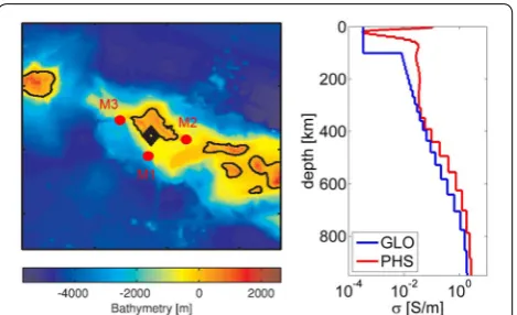
b, 1998, 2002; Pankratov et al. 1998, 2004; Pulkkinen and Engels 2005; Avdeev and Avdeeva 2009; Kalscheuer et al. 2012; Samrock and Kuvshinov 2013). The conduc-tivity model we adopted consists of eight anomalous layers (three layers account for topography and five for bathymetry) on top of a one-dimensional (1-D) conduc-tivity section. Bathymetry and topography data have been taken from the ETOPO1 Global Relief Model database (Amante and Eakins 2009). The left plot of Fig. 1 presents the map of bathymetry and topography in the region. The 3-D conductivity distribution within the eight anomalous (10)
layers is derived under the assumption of a seawater conductivity of σsea=3.2 S/m and a land conductivity of σland = 10−2 S/m. The original, one arc-minute, data of bathymetry and topography used for estimating con-ductivity distributions in these layers were interpolated to a regular Cartesian grid with a horizontal cell size of 1 km × 1 km. The total horizontal size of the model was 356 km × 356 km. The sensitivity of scalar responses to conductivity variations beneath ocean was investigated with respect to two different 1-D conductivity sections. These sections are shown in the right plot of Fig. 1. The first 1-D section, labeled as GLO, is a global conductiv-ity section that has been inferred from satellite magnetic data (Kuvshinov and Olsen 2006) and that was modified to have a realistic low conductivity in the upper 100 km as these depths are not resolvable by satellite magnetic data. The second 1-D section, denoted as PHS, is a regional 1-D model (for the Philippine Sea), which has been recovered from sea-floor MT data (Baba et al. 2010). Note that we performed extensive model studies to justify the param-eters describing the model (cell and mesh sizes, number of anomalous layers, values for seawater and land conduc-tivities). These studies revealed that the effects from vary-ing seawater and land conductivities are smaller than the effect from varying the 1-D section.
Figure 2 exemplifies surface maps of tipper, horizon-tal magnetic tensor and scalar magnetic response at the period of 1300 s for the region around Oahu Island, Hawaii. The left and right plots show the magnitudes of the real and imaginary parts of the corresponding
responses, respectively, which, in case of the scalar responses, are defined as
Similarly, we define RT, IT, RMx, IMx, RMy and IMy . Note that Honolulu magnetic observatory (IAGA code HON) was chosen as the reference site. Also note that here the global (GLO) 1-D conductivity profile was used as underlying 1-D section. Finally, we remark that the normalized static magnetic field p was calculated using a
recent update of the CHAOS model (Olsen et al. 2014). Figure 2 shows the anomalous behavior in both the real and imaginary parts of all responses in the regions where lateral contrasts of conductivity (here controlled by bathymetry) exist (the so-called coast or ocean effect discussed in numerous papers (Lilley et al. 1979; Lilley
2005; Kuvshinov and Utada 2010). The horizontal mag-netic tensor M and scalar magnetic response S reveal anomalous behavior offshore, whereas the most promi-nent anomalies of tipper T are confined to the coast. In general, it is seen that the scalar magnetic response S is indeed a combination of components of tipper and hori-zontal magnetic tensor.
It is also interesting to note that T (and thus total-field fluctuations) are suppressed on the north side of Oahu. This pattern is a nice example of magnetic amphidrome conditions, mentioned in “Scalar responses” section.
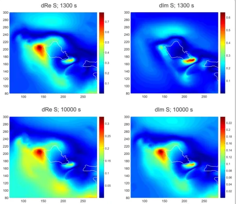
To quantify the sensitivity of scalar magnetic responses to subsurface conductivity we also compute the responses using a different, regional (PHS) 1-D conduc-tivity profile. The maps in Fig. 3 present the difference between scalar magnetic responses computed for the two 1-D sections. Here, the difference (in the real part) stands for the quantity
where superscripts “G” and “P” denote results obtained in the model with global (GLO) and regional (PHS) 1-D conductivity profiles, respectively. Similarly, we define the difference in the imaginary part. The results are presented for the two periods 1300 s (top) and 10,000 s (bottom). The difference is most prominent near the northwest and the southeast (offshore) tips of Oahu Island and reaches 50% of the responses themselves at a period of 1300 s (cf. the bottom plots in Fig. 2).
Final model experiment comprises computation of the responses using 1-D section which coincides with PHS profile down to depth of 14 km (the depth where GLO and PHS profiles meet; cf. right plot of 1) and follows GLO profile below 14 km. The maps of difference between the (14)
responses computed for this and GLO sections (see Addi-tional file 1) suggest that the scalar responses are most sensitive to the upper (crustal) layers of the 1-D section.
Scalar field measurements using the Wave Glider platform
From the model study we identified three regions around Oahu island where the largest sensitivity of scalar responses, as quantified by Eq. (15), to subsurface con-ductivity were detected. The actual location of the sites is shown in Fig. 1 by red dots. The coordinates of the sites, hereinafter denoted as M1, M2 and M3 sites, are (21.0835◦N, 158.0000◦W), (21.2420◦N, 157.6290◦W) and (21.5540◦N, 158.3821◦W), respectively.
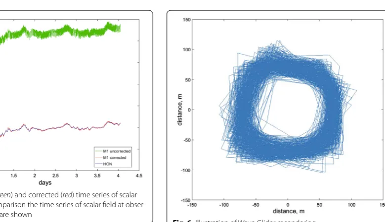
To measure the scalar magnetic field variations at these locations, the Wave Glider observation platform was used. The Wave Glider autonomous surface vehicle (ASV) was invented and developed by Liquid Robot-ics Inc. It is a two-part vehicle and comprises a surface component (the “float”; shown in the left plot of Fig. 4) and a submerged component (the “sub”; shown in the right plot of Fig. 4) connected by an umbilical tether. The ASVs propulsion system is passive and mechanical; it converts energy from wave motion into thrust. Solar pan-els mounted on the platform are used to charge batteries which provide power to the control system, radios and payload. Other components of the vehicle are a satellite communication system, navigation control, solar charg-ing system, batteries and different instrument payloads. In our experiment the Wave Glider was equipped with a towed scalar magnetometer model “Explorer” by Marine Magnetics, www.marinemagnetics.com. The control and communication with the vehicle is provided via a satellite system. The ASV can be programmed to travel directly from one location to another, follow a specific route, or can be fixed at one position (within ±200 m or so) for a long time (from days to weeks). In our marine survey, continuous measurements at fixed positions were con-ducted for 3.8, 2.9 and 8 days at the sites M1, M2 and M3, respectively. The scalar magnetic field measure-ments were performed in May–August of 2013, and syn-chronous measurements of the horizontal magnetic field from Honolulu magnetic observatory were used as refer-ence site data.
Data processing
site appeared to be due to ±200 m meandering of Wave Glider position (shown in Fig. 6) in the presence of strong gradients of crustal field which are observed in this region.
To suppress undesirable oscillations in the data we elaborated the following correction scheme.
• First, we subtract the CHAOS predictions of scalar static magnetic field from the data at both survey and reference site. We denote the resulting signals as
Fs(r(t),t) and Fb(rb,t), respectively. The dependence of r on time t in Fs reflects the fact that Wave Glider
slightly changes its position. This step removes the
observed offset between survey and reference meas-urements.
• Second, we subtract the Fb(rb,t) from Fs(r(t),t). The resulting part of the signal, denoted as δFs(r(t)) , should only contain observed oscillations at the sur-vey site which are associated with fluctuations of the Wave Glider position. This is true under the assump-tion that time variaassump-tions of the scalar magnetic field due to external source (of ionospheric or/and magne-tospheric origin) are approximately the same at sur-vey and reference site.
• Third, we approximate δFs by a bilinear function in
horizontal position x, y:
and determine the coefficients A, B, C and D by least squares fitting. Here, we introduce local two-dimen-sional (OXY) Cartesian coordinate system where the origin of coordinates coincides with the location of the reference site.
• Finally, once the coefficients A, B, C and D are deter-mined, we obtain corrected data, Fc(r,t), at survey site as
Red curve in Fig. 5 shows the corrected time series at M1 site obtained by implementing the above scheme. It is (16)
δFs(r(t))≈Ax(t)+By(t)+Cx(t)y(t)+D,
(17) Fc(r,t)=Fs(x(t),y(t),t)−(Ax(t)
+By(t)+Cx(t)y(t)+D).
seen from the figure that the correction scheme indeed suppresses high-frequency oscillations at survey site caused by small changes in position of the measuring platform.
Observed versus predicted responses
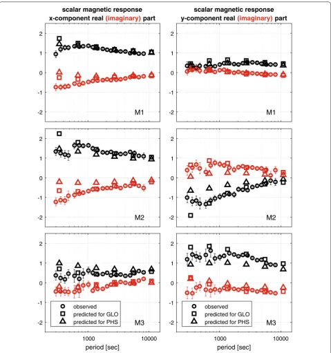
The six plots in Fig. 7 show the comparison of predicted and observed scalar magnetic responses. Left and right plots present the x- and y-components of the responses, respectively, with black and red colors showing real and imaginary parts. The observed responses were estimated using a data processing tool (Püthe and Kuvshinov 2014) based on a robust section-averaging approach with a jackknife estimator of the uncertainties.
Fig. 4 Two images of the Wave Glider. Right float; left float and sub during deployment. More images are at http://www.lrog.com/the-wave-glider/ gallery.html
Fig. 5 Uncorrected (green) and corrected (red) time series of scalar field at M1 site. For comparison the time series of scalar field at obser-vatory Honolulu (blue) are shown
It is seen from the figure that overall the predic-tions (squares—for GLO model, and triangles—for PHS model) are in encouraging agreement with the observations (open circles with error bars) at all sites, in both components, and in real as well as imagi-nary parts. Even the predicted reversal of the real and
imaginary parts of Sfy at M2 site is similar to the obser-vations. The remaining discrepancy is most probably due to inaccuracy of the underlying 3-D conductivity model, and partly due to inaccuracy in the estimated (observed) responses, due to the limited time length of observations.
-2 -1 0 1 2
scalar magnetic response x-component real (imaginary) part
M1 -2 -1 0 1 2
scalar magnetic response y-component real (imaginary) part
M1
-2 -1 0 1 2
M2 -2 -1 0 1 2
M2
1000 10000
period [sec] -2
-1 0 1 2
M3 observed
predicted for GLO predicted for PHS
1000 10000
period [sec] -2
-1 0 1 2
M3 observed
predicted for GLO predicted for PHS
Conclusions and discussion
In this paper we discuss a concept of marine induction surveying which is based on sea-surface scalar magnetic field measurements from a position-keeping platform. The concept exploits scalar magnetic responses that relate variations of the scalar magnetic field at the survey sites with variations of the horizontal magnetic field at a reference site. We demonstrate—based on a realistic 3-D model study—that the scalar magnetic responses are sen-sitive to the conductivity structures beneath the ocean. We conclude that the sensitivity, depending on the hori-zontal gradient of bathymetry, is typically largest near the coast offshore. We show that such sea-surface marine induction surveys can be performed with the Wave Glider observation platform. We believe that this type of survey represents an attractive complement to traditional marine MT studies based on sea-bottom vector measure-ments. We also would like to remark here that in contrast to sea-bottom observations, which require special design of the instruments, one can use standard instruments for the scalar survey.
Performing 3-D models studies we ultimately tested whether the observations are able to distinguish between two 1-D models that strongly differ down to 300 km depth. The topic for further work could include answer-ing the followanswer-ing questions: (a) What are the prospects of distinguishing between profiles which differ less? (b) Whether one can resolve 3-D inhomogeneities beneath oceans with this technique? (c) What is an optimal res-olution of the model to account properly for the ocean effect? (d) Is it possible to improve the quality of the observed responses?
As for survey concept itself, we are also aware of some drawbacks. First, since the scalar magnetic responses are a combination of components of tipper and horizontal magnetic tensor, they cannot contain any useful informa-tion about the Earth’s interior in regions characterized by a 1-D conductivity distribution. Indeed, assuming a vertically incidenting plane wave source and a 1-D con-ductivity, the tipper is zero and the horizontal magnetic tensor is just the unit matrix. Luckily in our survey setup one always has a 3-D environment due to the contrast between ocean and land (recall that a reference site is located onshore), and variable bathymetry.
Second, an estimation of the scalar magnetic responses requires measurements of the horizontal magnetic field components at a reference site. This means that the con-cept will only work in oceanic regions sufficiently close to a reference station (less than a few hundred kilometers to satisfy the source vertically incidenting plane wave approximation for both locations).
Third, the highly conducting ocean acts as an effec-tive shield, which prevents the electromagnetic field at
shorter periods to penetrate into the Earth; the deeper the ocean the stronger this shielding. Consequently, the shallower the ocean, the better the performance of the sea-surface scalar survey.
Lastly, one can speculate that on the sea surface the magnetic signals from waves and swells could affect the scalar response estimation. However, these motionally induced signals have much higher frequencies (Lilley et al. 2004) compared to the signals we are interested in.
In this paper we explore the applicability of the Wave Glider platform to measure signals originating from plane wave sources. Another option could be the use of the platform for measuring the solar-quiet (Sq) daily variations of the magnetic scalar field in remote oceanic regions otherwise not covered by observations. In this scenario, scalar measurements are analyzed together with simultaneous data from a global net of geomagnetic observatories by means of estimating and interpreting local-to-global responses, similar to those introduced in Püthe et al. (2014). Note that for this type of survey there is no need for reference site observations. One alert, however, is that there are bands of latitude (between dips I=20◦ and I=30◦, and between dips I= −20◦
and I= −30◦) where the scalar Sq signal is substantially
suppressed because the Sq field direction is largely per-pendicular to the main field direction (cf. the note after Eq. 4).
In contrast to sea-bottom MT observations, which include electric field measurements, our observations are purely magnetic, at least at the survey sites. As shown in Appendix 1, another type of responses could be con-structed which relate variations of the scalar magnetic field at the survey sites with variations of the horizontal electric field at a reference site. However, in this case the galvanic distortion problem (cf. Jiracek 1990) could com-plicate the interpretation.
has the advantage of leading to responses that contain information about the electric field at the survey site.
Abbreviations
MT: magnetotelluric; ASV: autonomous surface vehicle; USGS: United States Geological Survey.
Authors’ contributions
AK and JM initiated the study and wrote the draft, BP and SP conducted the Wave Glider survey, AK and FS performed the model study, and AK and NiO processed the data. All authors read and approved the final manuscript.
Author details
1 Institute of Geophysics, ETH, Zurich, Sonneggstrasse 5, 8092 Zurich, CH,
Switzerland. 2 GFZ German Research Centre for Geosciences, Telegrafenberg,
14473 Potsdam, Germany. 3 Schlumberger, 5599 San Felipe St, Houston, TX
77056, USA. 4 DTU Space, Technical University of Denmark, Diplomvej 371,
2800 Kgs. Lyngby, Denmark. 5 Liquid Robotics Oil and Gas, 5599 San Felipe St,
Houston, TX 77056, USA.
Acknowledgements
We thank USGS for validating the scalar magnetometer, and for providing magnetic data from the Honolulu observatory. We extend our special grati-tude to F.E.M. (Ted) Lilley who made many valuable comments on the manu-script and drew our attention on a number of seminal papers overlooked in the initial version of the manuscript.
Competing interests
The authors declare that they have no competing interests.
Appendix 1: Scalar mixed responses
Let us introduce the inter-site admittance Y which relates
variations of the horizontal magnetic field at a survey site with variations of the horizontal electric field at a refer-ence site
where EH =(Ex Ey). Similarly, as it was done in “Scalar responses” section, by substituting Eq. (18) in Eq. (5), and then substituting the resulting equation and Eq. (18) in Eq. (4) we obtain the desired relation
where the responses, Afx and Afy, which we will call
“sca-lar mixed responses,” are a combination of components of tipper T, elements of the admittance tensor Y and components of the normalized main field p
Additional file
Additional file 1: Figure S1. Difference between scalar magnetic responses for the two 1-D sections GLO and PHS + GLO at two peri-ods—1300 (top) and 10000 (bottom) sec. PHS + GLO section coincides with PHS profile down to depth of 14 km (the depth where GLO and PHS profiles meet; cf. right plot of Figure 1 of the main text) and follows GLO profile below 14 km. Left and right plots show the magnitude of the real and imaginary part of the corresponding difference, respectively. Note that different scales are used for the plots.
(18)
The first four statements in bullets in “Scalar responses” section on the scalar magnetic responses are also valid for these scalar mixed responses.
Appendix 2: Scalar gradient responses
Let us assume that variations of the scalar magnetic field are simultaneously measured at sea surface and directly below at a certain depth in the ocean. Also let us assume that the period of the variations is long enough to write
Here, superscripts “+” and “−” stand for sea surface and at depth, respectively, µ0 is the magnetic perme-ability of free space, n is an upward unit vector, S=σd is the conductance, where σ is (assumed to be known) conductivity of seawater, and d is depth. Then, using Eq. (22), we can write the vertical gradient of the scalar magnetic field as
or expressed via electric field (cf. Eq. 23) as
Here, pH =(px py). Substituting the inter-site imped-ance relation
in Eq. (25) we obtain responses that relate variations of the vertical gradient of the scalar magnetic field at a survey site with variations of the horizontal magnetic field at a reference site by
where the responses Vgx and Vgy, which we will call “sca-lar gradient magnetic responses,” are a combination of elements of inter-site impedance, conductance and normalized horizontal magnetic field
If the horizontal electric field is measured at a reference site, then alternative scalar gradient responses can be introduced that relate variations of the vertical gradient of the scalar magnetic field at a survey site with varia-tions of the horizontal electric field at a reference site
where the responses, Ugx and Ugy, which we will call “scalar gradient electric responses,” are a combination of elements of horizontal electric (telluric) tensor, con-ductance and normalized horizontal static field
Note that in order to obtain the latter equations we used the following relation
Received: 19 April 2016 Accepted: 26 October 2016
References
Amante C, Eakins BW (2009) ETOPO1 1 Arc-minute global relief model: proce-dures, data sources and analysis. US Department of Commerce, National Oceanic and Atmospheric Administration, National Environmental Satel-lite, Data, and Information Service, National Geophysical Data Center, Marine Geology and Geophysics Division, Boulder, CO, USA
Avdeev D, Kuvshinov A, Pankratov O (1994) On a module magnetovariational profiling. Phys Solid Earth 3:75–80
Avdeev D, Kuvshinov A, Pankratov O, Newman G (1997) High-performance three-dimensional electromagnetic modeling using modified Neumann series. Wide-band numerical solution and examples. J Geomagn Geo-electr 49:1519–1539
Avdeev D, Kuvshinov A, Pankratov O (1997) Tectonic process monitoring by variations of the geomagnetic field absolute intensity. Ann Geophys 40:281–285
Avdeev D, Kuvshinov A, Pankratov O, Newman GA (1998) Three-dimensional frequency-domain modelling of airborne electromagnetic responses. Explor Geophys 29:111–119
Avdeev DB, Kuvshinov AV, Pankratov OV, Newman GA (2002) Three-dimen-sional induction logging problems, part I: an integral equation solution and model comparisons. Geophysics 67(2):413–426
Avdeev DB, Avdeeva AD (2009) 3D magnetotelluric inversion using a limited-memory quasi-newton optimization. Geophysics 74:45–57
Baba K, Utada H, Goto T, Kasaya T, Shimizu H, Tada N (2010) Electrical con-ductivity imaging of the Philippine Sea upper mantle using seafloor magnetotelluric data. Phys Earth Planet Inter 183:44–62
Berdichevsky MN, Dmitriev VI (2008) Models and methods of magnetotellurics. Springer, Berlin
Chave AD, Jones AG (2012) The magnetotelluric method—theory and prac-tice. Cambridge University Press, Cambridge
Hitchman AP, Lilley FEM, Campbell WH (1998) The quiet daily variation in the total magnetic field: global curves. GRL 25:2007–2010
Hitchman AP, Lilley FEM, Milligan PR (2000) Induction arrows from offshore floating magnetometers using land reference data. GJI 140:442–452
(30)
Jiracek GR (1990) Near-surface and topographic distortions in electromagnetic induction. Surv Geophys 11:163–203
Kalscheuer T, Huebert J, Kuvshinov A, Lochbuehler T, Pedersen L (2012) A hybrid regularization scheme for the inversion of magnetotelluric data from natural and controlled sources to layer and distortion parameters. Geophysics 77:301–315
Key K, Constable S, Liu L, Pommier A (2013) Electrical image of passive mantle upwelling beneath the northern East Pacific Rise. Nature 495:499–502 Khan A, Shankland TJ (2012) A geophysical perspective on mantle water
content and melting: inverting electromagnetic sounding data using laboratory-based electrical conductivity profiles. Earth Planet Sci Lett 317, 318:27–43
Kuvshinov AV (2008) 3-D global induction in the oceans and solid Earth: recent progress in modeling magnetic and electric fields from sources of magnetospheric, ionospheric and oceanic origin. Surv Geophys 29(2):139–186. doi:10.1007/s10712-008-9045-z
Kuvshinov A, Olsen N (2006) A global model of mantle conductivity derived from 5 years of CHAMP, Ørsted, and SAC-C magnetic data. Geophys Res Lett 33(18):18301
Kuvshinov A, Utada H (2010) Anomaly of the geomagnetic Sq variation in Japan: effect from subterranean structure or the ocean effect? Geophys J Int 181:229–249
Lilley FEM, Hitchman AP, Milligan PR, Pedersen T (1979) The geomagnetic coast effect. Rev Geophys Space Phys 17:1999–2015
Lilley FEM, Sloane MN, Ferguson IJ (1984) A geophysical perspective on mantle water content and melting: inverting electromagnetic sounding data using laboratory-based electrical conductivity profiles. J Geomag Geoelectr 36:161–172
Lilley FEM, Hitchman AP, Wang LJ (1999) Time-varying effects in magnetic mapping: amphidromes, doldrums and induction hazard. Geophysics 64:1720–1729
Lilley FEM, Hitchman AP, Milligan PR, Pedersen T (2004) Sea-surface observa-tions of the magnetic signals of ocean swells. GJI 159:565–572 Lilley FEM (2005) Coast effect of induced currents. In: Gubbins D,
Herrero-Bervera E (eds) Encyclopedia of geomagnetism and paleomagnetism. Springer, Berlin, pp 61–65
Naif S, Key K, Constable S, Evans RL (2013) Melt-rich channel observed at the lithosphere-astenosphere boundary. Nature 495:356–359
Olsen N, Lühr H, Finlay CC, Sabaka TJ, Michaelis I, Rauberg J, Toffner-Clausen L (2014) The CHAOS-4 geomagnetic field model. Geophys J Int 197:815–827
Pankratov O, Avdeev D, Kuvshinov A (1995) Electromagnetic field scattering in a homogeneous Earth: a solution to the forward problem. Phys Solid Earth 31:201–209
Pankratov O, Avdeev D, Kuvshinov A, Shneyer V, Trofimov I (1998) Numerically modelling the ratio of cross-strait voltage to water transport for the Ber-ing Strait. Earth Planets Space 50(2):165–169. doi:10.1186/BF03352097 Pankratov O, Kuvshinov A, Avdeev D, Schneyer V, Trofimov I (2004) Ez-response
as a monitor a Baikal rift fault electrical resistivity: 3D model studies. Ann Geophys 47:151–156
Pulkkinen A, Engels M (2005) The role of 3D geomagnetic induction in the determination of the ionospheric currents from ground-based data. Ann Geophys 23:909–917
Püthe C, Kuvshinov A, Olsen N (2014) Handling complex source structures in global EM induction studies: from C-responses to new arrays of transfer functions. Geophys J Int 201:318–328
Püthe C, Kuvshinov A (2014) Mapping 3-D mantle electrical conductivity from space: a new 3-D inversion scheme based on analysis of matrix Q-responses. Geophys J Int 197:768–784