FRONTIER LETTER
In‑flight scalar calibration
and characterisation of the Swarm
magnetometry package
Lars Tøffner‑Clausen
1*, Vincent Lesur
2, Nils Olsen
1and Christopher C. Finlay
1Abstract
We present the in‑flight scalar calibration and characterisation of the Swarm magnetometry package consisting of the absolute scalar magnetometer, the vector magnetometer, and the spacecraft structure supporting the instruments. A significant improvement in the scalar residuals between the pairs of magnetometers is demonstrated, confirming the high performance of these instruments. The results presented here, including the characterisation of a Sun‑driven disturbance field, form the basis of the correction of the magnetic vector measurements from Swarm which is applied to the Swarm Level 1b magnetic data.
Keywords: Geomagnetism, Magnetometer, Instrument calibration, Satellite, Swarm
© 2016 The Author(s). This article is distributed under the terms of the Creative Commons Attribution 4.0 International License (http://creativecommons.org/licenses/by/4.0/), which permits unrestricted use, distribution, and reproduction in any medium, provided you give appropriate credit to the original author(s) and the source, provide a link to the Creative Commons license, and indicate if changes were made.
Introduction
In November 2013 the European Space Agency (ESA) launched the three Swarm satellites, named Alpha, Bravo, and Charlie, with the objective to provide the best ever survey of the geomagnetic field and its tempo-ral evolution (Friis-Christensen et al. 2006). Each space-craft carries an Absolute Scalar Magnetometer (ASM) for measuring Earth’s magnetic field intensity, a Vector Fluxgate Magnetometer (VFM) measuring the direc-tion and strength of the magnetic field, and a three-head Star TRacker (STR) mounted close to the VFM to obtain the attitude needed to transform the vector readings to an Earth-fixed coordinate frame. Time and position are provided by an on-board GPS receiver. The payload also includes instruments to measure plasma and electric field parameters as well as non-gravitational acceleration.
One of the purposes of the scalar magnetometer (ASM) is to provide the necessary absolute magnetic data to calibrate the vector magnetometer (VFM). For this an approach similar to that adopted for the previous satel-lite missions Ørsted and CHAMP was foreseen (c.f. Olsen
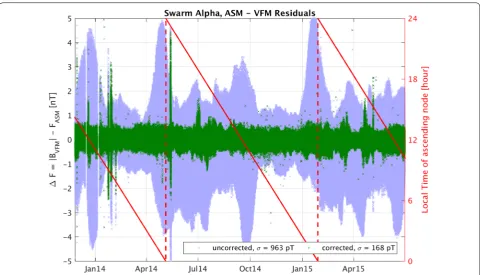
2003; Yin and Lühr 2011) since those missions carried equivalent instrumentation. However, soon after launch of Swarm it became clear that the magnetic field vector measurements on all three spacecraft were contaminated by unforeseen disturbances which could not be captured by the traditional in-flight calibration methods referred to above. Furthermore, the disturbances show systematic variation which could impact or map into scientific inves-tigations based on Swarm magnetic data. The light blue symbols in Fig. 1 show time series of the scalar residuals, which are the difference, F = |�BVFM| −FASM, between the modulus of the VFM data, |�BVFM|, and the magnetic
intensity measurements, FASM, taken by the ASM
instru-ment. Based on experience with Ørsted and CHAMP sca-lar residuals with sub-nanotesla level were expected (rms value well below 0.5 nT), while for Swarm the scatter of the residuals was observed to reach several nT, resulting in an rms value approaching 1 nT, but crucially showing a very clear local time dependence. A task force was there-fore established to investigate and mitigate the effect.
Detailed investigations of the scalar residuals F and of the ASM and VFM measurements separately indicated that:
• the vector readings of the VFM are affected by a dis-turbance vector field;
Open Access
*Correspondence: [email protected]
1 Division of Geomagnetism, DTU Space, Technical University of Denmark, Diplomvej, Kongens Lyngby, Denmark
• the scalar readings of the ASM are much less, if at all, affected.
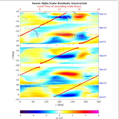
Consequently, the task force concluded to pursue models which assume the magnetic disturbance to be affecting the VFM measurements only. Plotting F as a function of the Sun incidence angles with respect to the space-craft, reveals systematic features of the disturbance, as shown in Fig. 2. At the start of “Characterisation and cali-bration with scalar residuals” section we provide detailed definitions of the two Sun incidence angles α and β. This
supports the hypothesis that a magnetic source in the vicinity of the VFM magnetometer, with strength and direction depending on the direction to the Sun (as seen from the spacecraft), is responsible. We refer to such a disturbance field vector that depends on the direction to the Sun, as δBSun.
The purpose of this article is to document the details of in-flight calibration of the Swarm magnetometer pack-age, including an empirical determination and removal of the Sun-driven vector disturbance field δBSun, based on
a mitigation approach proposed by Vincent Lesur (Lesur et al. 2015).
“Characterisation and calibration with scalar residu-als” section describes the parameterisation of the model of the Sun-driven disturbance—in following referred to
as the characterisation of the disturbance field—and of the calibration of the VFM instrument, by which means determination of its intrinsic scale factors and their dependence on time and temperature, and determina-tion of the sensor-axis non-orthogonalities. We docu-ment the adopted Iteratively Reweighted Least Squared (IRLS) estimation approach that includes a truncated sin-gular value decomposition (SVD) approach to solving the inverse problem. The results obtained for Swarm Alpha, based on data covering the period from launch (22 November 2013) until end of June 2015 (i.e. 19 months), are presented in “Results of model estimation for Swarm Alpha” section. Application of the scheme to data from the satellites Bravo and Charlie resulted in similar levels of residual improvement and statistics, and the estimates of the Sun-driven disturbance δBSun show generally
simi-lar behaviour and structural features as found for Swarm Alpha, although there are also some differences. Finally, “Conclusions” section summarises the findings and pro-vides perspectives regarding further improvements of the method.
Characterisation and calibration with scalar residuals
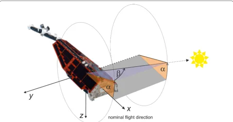
The Sun incidence angles α and β are crucial in our
approach to characterise the scalar residual. To clarify,
in Fig. 3 we illustrate the definition of these angles with respect to the spacecraft and the Sun position. α
is the azimuth in the spacecraft x–z plane (nominally the orbit plane), and β is the “elevation” out of the x–z
plane positive towards left (looking in the nominal flight direction; i.e. positive opposite the spacecraft y-axis). Examples of values for α and β for particular
Sun positions are:
• β= +90◦: Sun directly from −y (i.e. from the left
during nominal flight)
• β= −90◦: Sun directly from +y (i.e. from the right)
• β=0◦, α=0◦: Sun directly from +x (i.e. from the front)
• β=0◦, α= +90◦: Sun directly from −z (above)
• β=0◦, α= +180◦: Sun directly from −x (i.e. from the back—slightly above the boom)
Considering how these angles vary over orbits of the Swarm spacecraft during nominal flight, we find that α
varies rapidly from 360◦ down to 0◦ within one orbit (i.e. within ≈90 min), while β varies slowly up and down
typi-cally by ≈1.25◦ in one day (for Alpha and Charlie, 1.20◦
for Bravo).
Although the observed scalar residuals clearly vary with the Sun incidence angles α and β (see Fig. 2), there is no
direct mapping of F in terms of these parameters. This is a consequence of the scalar residuals �F≈δB�Sun· �b0
being the projection of the magnetic disturbance vector
δBSun, onto the unit vector b0 of the ambient magnetic
field direction (Earth’s main field). The former is oriented relative to the spacecraft, while the latter is oriented rela-tive to Earth, which results in the variations with the spacecraft local time (captured by β) as seen in Fig. 2. The
spacecraft local time changes by 12 hours (corresponding to a change in β by 180◦) within approximately 412 months.
To account for the projection on to the ambient field, we consider a vector magnetic disturbance δBSun(α,β) , with each component depending individually on the Sun incidence angles. Mathematically, we describe each component of the disturbance field vector by a spheri-cal harmonic expansion in α and β i.e. we consider three
independent spherical harmonic expansions in all.
This model characterising the Sun-driven disturbance is co-estimated together with a model of the temporal evolution of the VFM sensitivity and an adjustment of the pre-flight estimated non-orthogonality angles of the VFM sensor. For this we perform a scalar calibration via a least squares fit, minimising the discrepancy (F) between the fully calibrated and corrected measurements from the ASM and the modulus of the vector measure-ments from the VFM after our model has been applied. Huber weights are used iteratively to eliminate the effect of anomalous measurements (“outliers”) on the estimated models.
Model parameterisation
As outlined above, our model characterising the Sun-driven disturbance vector δBSun consists of three
spheri-cal harmonic expansions up to degree and order 25, one for each of the magnetic field components in the VFM magnetometer frame, with the position of the Sun with respect to the spacecraft parameterised by the Sun inci-dence angles α and β. It takes the form
δB�Sun= 25
n=0 n
m=0
�
umn cosmα+ �vnmsinmα
Pmn(sinβ)
where umn and vmn are the spherical harmonic expan-sion coefficients, with one component for each compo-nent of the disturbance field, and Pnm are the Schmidt semi-normalised Legendre functions. Note that δBSun
includes static terms (n=m=0) that describe a static (i.e. independent of the Sun position) disturbance vector. The disturbance field vector δBSun is thus described by 3×262=2028 model coefficients.
The model for re-scaling the vector measurements and taking into account any small adjustment of the non-orthogonality of the VFM sensors, which is required in order to obtain the fully calibrated and corrected vector field measurements BVFM, now takes the form
where Bpre-flight are the VFM measurements calibrated
using the pre-flight parameters and corrected for the pre-flight determined stray fields as described in Tøffner-Clausen (2015). S is a 3×3 diagonal scaling matrix with elements
where sB-spline(t) is a quadratic B-spline in time with 3-month knot separation (common for all three com-ponents of the magnetic field), and sj,Tsensor,j=1−3 is an adjustment of the pre-flight estimated dependency of the VFM sensitivity on its sensor temperature, Tsensor , for each sensor axis j. sj,β is an empirical scaling
param-eter and β the Sun incidence angle, as defined above. The
choice of quadratic B-splines with 3-month knot separa-tion is made to allow sufficient flexibility of the model; the exact choice of B-spline knot times is not crucial as very similar results are obtained with other, similar parameterisations. The estimated B-splines exhibit very moderate accelerations (in the case of the full model, see Fig. 6), and it may be possible to simplify the parameteri-sation of the time dependence in future models, e.g. to an exponential saturation in time as this is the expected behaviour of the VFM instrument sensitivity; however, an exponential model is ill-conditioned on the time span of data used here.
P is the non-orthogonality matrix that makes small
adjustments to the pre-flight estimated non-orthogonal-ities of the VFM sensor (cf. Olsen 2003)
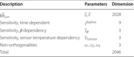
Our in-flight calibration model comprises 18 parameters in all; together with the 2028 parameters describing δBSun
�
this results in 2046 model parameters to be estimated, as listed in Table 1.
Estimation of model parameters: inversion and regularisation
In order to estimate the 2046 model parameters from the scalar residuals we need to solve a nonlinear inverse problem. The nonlinearity arises from the treatment of non-orthogonalities (Olsen 2003).
The forward relationship between the vector of the scalar residuals, d (di =Fi, the scalar residual of the ith data point), and the model parameter vector m, may therefore be written in the form
where g(m) is a nonlinear function of the model param-eters and e is a small remainder that cannot be explained by the model, which we seek to minimise.
Linearisation of this problem is straightforward. A reg-ularised, iteratively reweighted, least squares solution to the inverse problem is then obtained using the algorithm
where at the kth iteration, Gk = ∂g(m)∂m m=m
k, is the
appropriate Jacobian matrix, R is a regularisation matrix
discussed in detail below, and Wk is a (Huber) weighting
matrix.
Wk is updated at each iteration and consists of diagonal
elements
Table 1 Model parameters
Description Parameters Dimension
δBSun u,v 2028
Sensitivity, time dependent sBspline 9 Sensitivity, β dependency sβ 3 Sensitivity, sensor temperature dependency sTsensor 3 Non‑orthogonalities u1,u2,u3 3
being a (robust) estimate of the standard deviation of the residuals at iteration k. We set c=2, slightly higher than
the value of 1.5 usually chosen, in order to ensure that the less numerous polar data are not overly downweighted in the determination of the calibration parameters.
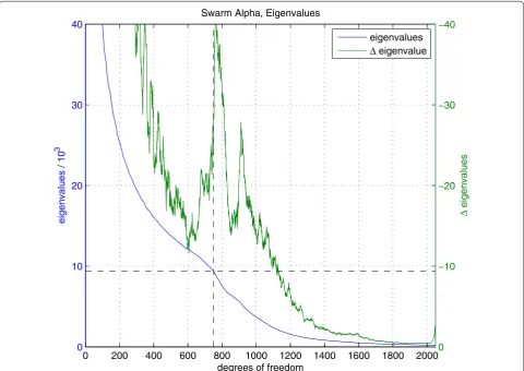
It turns out that the full set of 2046 parameters is not needed to obtain good results and low data misfit, which is confirmed by inspection of the eigenvalues of the matrix (GTkWkGk+R), as presented in Fig. 4 for Swarm Alpha. The magnitudes of the sorted eigenval-ues (in order of decreasing magnitude) exhibit a distinct drop around 750–800 degrees of freedom, indicating the smaller eigenvalues contribute little to the solution. The inversion of this matrix was therefore finally performed using a truncated singular value decomposition (TSVD) procedure, retaining only 750 degrees of freedom.
A regularisation matrix R is also included to help
stabilise the inversion. This is necessary because the Swarm satellites operate in a tightly controlled attitude
orientation which leads to a poor excitation of the VFM instrument along the axis perpendicular to the orbit plane (the east–west direction corresponding to the y-axis of the VFM sensor). Consequently, the parameters related to the y-axis are poorly determined in a scalar calibration. The regularisation matrix R is therefore defined so that it
acts on the parameters s2,Tsensor, s2,β, u1, and u3 to force s2,Tsensor≃s1,Tsensor+s3,Tsensor/2 (to reflect the physi-cal properties of the VFM sensor) and also to minimise the norms s22,β and u21+u23. is chosen to be sufficiently large to effectively impose the regularisation on the esti-mated model. Note that no regularisation is directly imposed on δBSun but use of truncated SVD during the
inversion automatically acts to suppresses structure in regions that are not well constrained by the input data.
The starting model for the inversions is “unity”, i.e. P=S=I, where I is the identity matrix, and �
umn = �vmn = �0. The inversions typically converge within 25 iterations.
0 10 20 30 40
degrees of freedom
eigenvalues / 10
3
Swarm Alpha, Eigenvalues
0 200 400 600 800 1000 1200 1400 1600 1800 20000
−10 −20 −30 −40
∆
eigenvalues
eigenvalues
∆ eigenvalue
Results of model estimation for Swarm Alpha
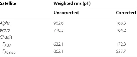
The model described above is estimated for Swarm Alpha using data from the beginning of the mission (22 Novem-ber 2013) until June 2015. Figure 1 shows the final scalar residuals, i.e. the residuals after application of the model (after “calibration and correction”) of the VFM measure-ments (in green), as a function of time together with the residuals of the un-corrected but re-scaled vector field measurements, i.e. B�VFM+δB�Sun, in light blue; these data illustrate what can be achieved with the traditional scalar calibration methods. Note the excellent reduction of the scalar residuals achieved by the model; the Huber weighted rms of the residuals drops from 963 to 168 pT. Table 2 pro-vides the corresponding numbers for Bravo and Charlie.
Figure 5 shows normal distribution plots for the scalar residuals. The top plot shows the distributions of all data for un-corrected (red) and fully corrected data (green) and demonstrates a transition from a non-Gaussian to Gaussian residual distribution when applying the model. The bottom plots show the distributions of the data split into 3-month periods, un-corrected to the left and cor-rected to the right. These also demonstrate the elimina-tion of systematic and non-Gaussian effects.
Table 3 lists the estimated sTsensor and sβ parameters
and the non-orthogonality values for all three Swarm satellites together with their estimated pre-flight values for the VFM instrument itself for reference. I.e. the table shows the adjustments applied in order to reduce the sca-lar residuals to the level indicated above.
Table 4 shows the increase in the weighted rms of the scalar residuals when omitting individual parts of the model—a full re-estimation of the remaining model
parameters is carried out for each table entry. Particu-larly the omission of the non-orthogonalities drasti-cally increases the misfit—the power (the mean-square) is more than doubled. Due to the stable attitude of the Swarm satellites, the small x–z non-orthogonality angle, u2, is equivalent to first order to a small, relative timeshift
between the ASM and VFM measurements—1 arc-sec-ond corresparc-sec-onds roughly to a 3-ms timeshift, and it has been discussed whether it would be more reasonable to introduce such timeshifts rather than adjusting the pre-flight estimated non-orthogonalities. However, the varia-tions in the u2 angles estimated by this model would imply
time-shifts varying from −3 ms to +13 ms for the individ-ual satellites which, to the authors, seems quite unlikely.
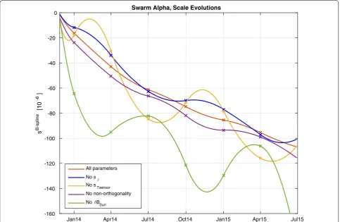
The temporal evolution of the scaling of the vector field measurements, sB-spline, is shown in Fig. 6 for the various
test models listed in Table 4. The full model, shown in red, shows a smooth behaviour in time, as expected from an instrument design perspective. The blue curve shows the model without sβ; this exhibits some small
oscilla-tions, whereas the light brown (no sTsensor) and green
(no δBSun) curves show much higher level of oscillations
indicating they are inadequate to capture the behaviour of the measurements. The elimination of the oscillations in the full model is a good indicator of the validity of this model. The magenta curve shows the model without non-orthogonalities; this is rather close to the curve of the full model and indicates the decoupling of the non-orthogonalities from any long-term temporal effect of the measurement disturbances and instruments.
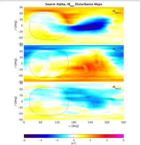
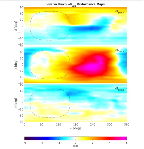
Maps of the three components of the estimated dis-turbance fields from the full model as function of Sun incidence angles α (abscissa) and β (ordinate) are given
in Figs. 7, 8, and 9 for Swarm Alpha, Bravo, and Char-lie, respectively. During nominal flight, the Sun inci-dence angles traverse these plots horizontally from right to left and move up or down in β as the orbit plane
moves through local time. The Sun-induced disturbance is observed to have temporal characteristics that are observed in the plots as horizontally stretched features, and these are attributed to thermal capacitance: The Sun-induced disturbance exhibits characteristic warm-up and cool-down effects, i.e. the disturbance increases when the spacecraft is exposed to the Sun, and decreases when the Sun exposure terminates. The time constants for these effects are up to tens of minutes (corresponding to sev-eral tens of degrees in the α angle). This effect is captured
Table 2 Scalar residual statistics, uncorrected, and cor-rected data
For Swarm Charlie two sets of numbers are given: one set for which the ASM was still working (FASM, until 5 November 2014) and one set using the scalar data
from Swarm Alpha mapped to the position of Swarm Charlie (FAC,map). For data
from 1 May 2014 through 5 November 2014 the weighted rms of FASM−FAC,map
−5 −4 −3 −2 −1 0 1 2 3 4 5
Fig. 5 Normal distribution plots of scalar residuals. Top all data, uncorrected (red), and corrected (green); the limits corresponding to the Huber weights (for corrected data) are shown by the vertical dashed lines. Bottom distributions split into quarters, uncorrected (left), and corrected (right), respectively
Table 3 Estimated values for selected model parameters for all three Swarm satellites
The nT-equivalents of the adjustments in a 50,000 nT ambient field are: sTsensor=10−6/◦C∼1.25 nT (25◦C temperature swing), sβ=0.1×10⁻⁶/deg∼ ±0.45 nT
(±90◦), u=1 arc−second∼0.242 nT
Sat Sensitivity/sensor temperature, sTsensor (10−6/◦C)
Sensitivity/β angle, sβ (10−6/deg) Non-orthogonalities, u1,2,3 (arc-seconds)
Pre-flight Adjustment Pre-flight Adjustment Pre-flight Adjustment
Alpha 28.5 0.616 – −0.125 102.386 −0.601
28.8 0.780 – 0 217.403 −3.960
28.3 0.945 – 0.012 −179.318 0.149
Bravo 28.3 1.168 – −0.132 350.880 −0.558
29.0 1.385 – −0.003 62.432 −2.453
28.8 1.602 – −0.198 −147.060 1.608
Charlie 27.7 1.521 – −0.090 139.140 0.094
29.1 1.300 – −0.038 −248.890 1.042
by the spherical harmonic model expansion of δBSun and
yields the horizontally stretched features in Figs. 7, 8, and 9. Note also the regions of nightside data (eclipse), the circled areas to the left of the figures, which generally
show less disturbance; this is not imposed by the model or any regularisation; rather, it is simply a result of the data itself and thus another indicator of the ability of the model to describe the observed disturbances. The plots also show both the similarities and the differences in
δBSun between the three satellites.
Conclusions
We have established a predominantly empirical model for the calibration and correction of the magnetic vec-tor field measurements of the three Swarm spacecraft. The model is based on detailed studies of the observed scalar residuals between the measurements of the abso-lute scalar magnetometer, ASM, and the modulus of the measurements of the vector field magnetometer, VFM. The model has proven to be quite robust as more data are incorporated into the estimation of the model Table 4 Weighted rms values for various models, Swarm
Alpha
Model Weighted rms (pT) Residual power (normalised) (%)
Full model 168.3 100
No sβ 176.1 107
No sTsensor 181.7 116 No non‑orthogonalities 250.2 221
No δBSun 962.6 3269
Jan14 Apr14 Jul14 Oct14 Jan15 Apr15 Jul15 -160
-140 -120 -100 -80 -60 -40 -20 0
s
B-spline
[10
-6 ]
Swarm Alpha, Scale Evolutions
All parameters No sβ No sTsensor No non-orthogonality NoδBSun
parameters, although the ambiguity of determining vec-tor disturbances from a pure scalar calibration affects the estimated correction vectors; these corrections do change slightly (by a few tenths of a nT) as more data are added.
The estimated models reduce the scalar differences between the Swarm magnetometers to generally below
0.5 nT with rms values well below 200 pT for all three sat-ellites and have been in operational use since April 2015 to produce corrected Swarm Level 1b magnetic field vec-tor data (as of version 0401).
Future evolutions of the model presented here are foreseen to include changing the model of the tempo-ral evolution of the VFM sensitivity from B-splines to
an exponentially decaying function. Analysis of δBSun
also indicates that this vector is generally confined to a few, distinct directions which may be incorporated in future models. Finally, it may be possible to model
the effect of the thermal capacitance using appropri-ate temporal filter functions which would lead to a sig-nificant reduction of the number of parameters of the model.
Data availability
The estimated disturbance vectors, δBSun, are included in
the operational Level 1b magnetic Swarm data products as dB_Sun.
Uncorrected data are available at ftp://swarm-diss. eo.esa.int/Advanced/ (login required, access can be requested via https://earth.esa.int/Swarm).
Authors’ contributions
LTC carried out the in‑flight scalar calibration and characterisation, analysed the results, and led the writing of this manuscript. VL proposed the model for the Sun‑induced vector disturbance, δBSun, and made the first estimations using this model. NiO and CF supported the entire project with many discus‑ sions, suggestions, and source code. All authors read and approved the final manuscript.
Author details
1 Division of Geomagnetism, DTU Space, Technical University of Denmark, Diplomvej, Kongens Lyngby, Denmark. 2 National Magnetic Observatory Geo‑ magnetism, Institut de Physique du Globe de Paris, 1 rue Jussieu, Paris, France.
Acknowledgements
We would like to thank ESA for establishing and providing support to the ASM‑VFM Task Force with the aim of investigating the source of the scalar residuals observed in the Swarm magnetic measurements and developing a correction scheme. We would also like to thank this Task Force for its work in characterising the behaviour of the magnetic disturbance and for many fruit‑ ful discussions and inputs for this work. In particular, we would like to thank Peter Brauer from the VFM instrument team for detailed discussions on the modelling and on the characteristics of the VFM instruments. Two anonymous reviewers are thanked for their comments that helped to improve the clarity of the manuscript. This paper is the IPGP contribution 3761.
Competing interests
The authors declare that they have no competing interests.
Received: 29 January 2016 Accepted: 29 June 2016
References
Friis‑Christensen E, Lühr H, Hulot G (2006) Swarm: a constellation to study the Earth’s magnetic field. Earth Planets Space 58:351–358
Lesur V, Rother M, Wardinski I, Schachtschneider R, Hamoudi M, Chambodut A (2015) Parent magnetic field models for the IGRF‑12 GFZ‑candidates. Earth Planets Space. doi:10.1186/s40623‑015‑0239‑6
Olsen N et al (2003) Calibration of the Ørsted vector magnetometer. Earth Planets Space 55:11–18
Tøffner‑Clausen L (2015), Swarm Level 1b processor algorithms. Esa doc. sw‑rs‑ dsc‑sy‑0002, National Space Institute, DTU Space, Copenhagen Yin F, Lühr H (2011) Recalibration of the CHAMP satellite magnetic field meas‑