Article
1
Analytical Solutions for the Propagation of
2
UltraShort and UltraSharp Pulses in Dispersive
3
Media
4
Er'el Granot1,*
5
1 Department of Electrical and Electronic Engineering, Ariel University, Ariel, Israel; [email protected]
6
* Correspondence: [email protected]
7
8
9
Abstract: Ultrashort pulses are severely distorted even by low dispersive media. While the
10
mathematical analysis of dispersion is well known, the technical literature focuses on pulses, which
11
keep their shape: Gaussian and Airy pulses. However, the cases where the shape of the pulse is
12
unaffected by dispersion is the exception rather than the norm. It is the object of this chapter to
13
present a variety of pulses profiles, which have analytical expressions but can simulate real-physical
14
pulses with greater accuracy. In particular, the dynamics of smooth rectangular pulses, physical
15
Nyquist-Sinc pulses, and slowly rising but sharply decaying ones (and vice-versa) are presented.
16
Besides the usage of this chapter as a handbook of analytical expressions for pulses' propagations in a dispersive
17
medium, there are several new findings. The main ones are: Analytical expressions for the propagation of
18
chirped rectangular pulses, which converge to extremely short pulses; analytical approximation for the
19
propagation of Super-Gaussian pulses; the propagation of Nyquist Sinc Pulse with smooth spectral boundaries
20
and an analytical expression for a physical realization of an attenuation compensating Airy pulse.
21
22
Keywords: Ultrashort pulses, Dispersion, Pulse distortion, optical communications
23
24
1. Introduction
25
Ultrashort pulses are ubiquitous in numerous applications: In bio- and medical-imaging (see, for example,
26
[1-3]), optical communications (see, for example, [4,5]), microscopy (see, for example, [6,7)], etc.
27
One of the clear shortcomings of short pulses is the consequences of their wide spectrum. When the
28
spectrum is spectrally wide, the absorption variations within the spectrum increases. However, even if the
29
absorption is approximately homogenous within the pulse spectral range, the refraction index is wavelength
30
dependent and therefore the pulse experiences dispersion effects.
31
Dispersion occurs whenever each one of the pulse's spectral components propagates with a different
32
velocity. Consequently, the pulse experiences shape distortions. The temporally shorter the pulse, the larger are
33
the distortions. Moreover, while the dispersion effects are proportional to the medium's length, it is inversely
34
proportional to the square of the pulse's temporal width; therefore, ultra-short pulses are prone to be affected by
35
dispersion even in relatively short media[8-10].
36
Clearly, most of the dispersion mitigation techniques were implemented in the optical communication
37
arena, where dispersion can have a destructive effect on the transmitting signals. It has been shown that via
38
ordinary smf28 fiber (the most ubiquitous fiber type) it is impossible to decode data, which is transmitted at a
39
10Gb/s rate, beyond a distance of 160km (see Ref.[11] and in the quantum analogy see Ref.[12]). Clearly, in the
40
presence of noise, this distance shrinks substantially. If the data is carried by picosecond pulses (which is only
41
1% of the temporal width of the 10Gb/s signal's individual pulses) this maximum distance is reduced to merely
42
16m, and the distortion effects will be felt within less than a meter. In the femtosecond domain, the dispersion
43
effects are, using the terminology and example of Ref.[13], more dramatic: a 10fs laser pulse in the 800nm
44
spectral regime, which propagate through a 4mm of BK7 glass will be temporally broadened to 50fs!
45
46
It is well known that dispersion is governed by the dispersion equation, which can easily be solved
47
numerically. However, to evaluate the effects of dispersion and to predict them, some intuition is required. In
48
most textbooks, Gaussian pulses are used as a litmus tool to predict the dispersion effect[8,13,14]. Gaussian
49
pulses are very useful since, on the one hand, they are localized pulses with a well-defined width and energy,
50
and on the other hand, the shape of their spectrum is mathematically similar to the dispersion effect. Therefore,
51
the propagation of Gaussian pulses in dispersion medium has a relatively simple analytical solution. This simple
52
pulse model can be used to evaluate qualitatively some fundamental limitations. However, it fails in quantifying
53
their values (see Ref.[11] and references therein). In fact, the Gaussian model predicts that the pulse keeps its
54
Gaussian shape, and its width is proportional to the square root of the elapsed period. This conduct resembles
55
the spatial spreading of a Gaussian distribution of particles in a diffusion process[15]. Since the "particle"
56
realization of the dispersion process is common in the popular description of chromatic dispersion, the
57
similarity to diffusion may be misleading, since, in fact, this similarity appears only in the Gaussian scenario.
58
Whenever the initial pulse profile deviates from the Gaussian's one, the differences between diffusion and
59
dispersion are clearly shown. In general, the two processes tend to smooth out the signal. However, the
60
processes are fundamentally different, and the main differences appear after short distances. This discrepancy
61
clearly appears in most optical communication protocols, where the pulses never have Gaussian profiles.
62
Consequently, the signal distortion is completely different from the Gaussian analysis predictions. To overcome
63
this problem, super Gaussian pulses are commonly used to model real communications scenarios [16-18].
64
Despite the fact that super Gaussian are much better approximation to real pulses, they have two weaknesses:
65
they cannot be implemented in Non-Return-to-Zero (NRZ) protocols and they do not have a close-form
66
analytical solution.
67
It is the object of this chapter to assemble important pulses profile, whose propagation in dispersive
68
medium can be expressed in analytical terms. It is shown that there are profiles, which are much better
69
candidates to simulate real pulses, but their dynamics can be formulated in a closed-form analytical expressions.
70
Moreover, it is shown that the dynamics of almost any practical pulse profile in dispersive media can be
71
simulated and approximated by analytical expressions.
72
73
74
In the 1st part of the chapter, after the introduction of the general theory (sec.2) and the presentation of
75
fundamental theorems (sec.3), the propagation of a Gaussian pulse is presented (sec. 4). In the 2nd part, it is
76
shown that it is possible to present analytically the propagation of singular pulses (sec. 5), which can be written
77
initially with exponentials and step functions (like rectangular pulses and exponential-step pulses). In the 3rd
78
pulse, which is presented in the previous part, can be replaced with its counterpart smooth version (sec. 6). In
80
particular, smooth rectangular pulses can replace super Gaussian ones. The 4th part is dedicated to the important
81
pulse, which is singular in the spectral domain, i.e., the Nyquist-Sinc pulse (sec. 7). First the analytical
82
expression for its propagation in dispersive medium is presented, and then the analytical expression of the
83
propagation of its spectrally-smooth, i.e., physical, counterpart is presented as well. In the last part of the
84
chapter, accelerated-airy pulses and attenuation compensating pulses are presented, as well as their physical
85
counterparts (sec 8).
86
87
88
2. Generic Dispersion Analysis
89
Let A
( )
t, represents the envelope of an electromagnetic (EM) pulse, which propagates in the z-direction z90
in a dispersive medium with the dispersion coefficient β2, then A
( )
t, obeys the following equation [14] z91
92
( )
( )
2 2
2 ,
2 ,
t z t A z
z t A i
∂ ∂ β = ∂
∂ (1)
93
where t=t'−z/v is the time in a frame of reference that travels at the velocity of light in the medium
94
(v=c/n, where c is the vacuum light's velocity and n is the mean refractive index), i.e., t' is the real
95
time. This equation is valid provided all spectral components of the pulse are governed by the following
96
dispersion relation
97
k c
nω+β2ω2 =
2 (2)
98
If A
( )
t,0 is the initial pulse profile, then the pulse profile at the end of the medium A( )
t, can be evaluated z99
by the following convolution
100
( )
t,z K(
t t,'z) ( )
At,'0dt'A
∞
∞ −
−
= (3)
101
where the dispersion Kernel (see Appendix A) is
102
(
) (
)
( )
β − − β
π − =
− −
z t t i z
i z
t t K
2 2 2
/ 1 2
2 ' exp
2
,' (4)
103
3. Fundamental Dispersion Theorems
104
To analyze the dispersion dynamics of the different pulses, we need some analytical tools, which will be
105
formulated as the following theorems.
106
3.1. Pulse Boosting and Decaying
107
Let A
( )
t,0 be an initial pulse whose dispersive dynamics is known, i.e., at the end of the dispersive medium its108
profile is also given A
( )
t, . Then, if the initial pulse is boosted by shifting the pulse's spectrum, i.e., by z109
multiplying the profile by an harmonic function
110
(
, 0)
exp(
) ( )
,0' t z i 0t At
A = = ω (5)
111
(
t z)
i z i t A(
t z z)
A ,
2 exp 0 ,
' 2 0 2 0
0
2 +β ω
ω + ω β =
> . (6)
113
Clearly, this theorem can be generalized to the case where the initial pulse is multiplied by an exponent
114
(
, 0)
exp( ) ( )
,0't z atAt
A = = (7)
115
where a can be any real, imaginary or complex number. In which case, if the initial function does no diverge,
116
the solution at the end of the medium is
117
(
t z)
i a z at A(
t i az z)
A ,
2 exp 0 ,
' 2 2 − β2
+ β − =
> (8)
118
3.2 Pulse Chirping
119
Let A
( )
t,0 be an initial pulse whose dispersive dynamics is known, i.e., at the end of the dispersive medium its120
profile is A
( )
t, , then, if the initial pulse is chirped, i.e., z121
( )
,0 exp(
)
( )
,0't iqt2 At
A = − (9)
122
for any real q, the pulse's profile at the end of the medium (after a distance z) is (see Appendix C)
123
( )
(
)
β + β +
+ β − β
+
= −
zq z zq t A q z
t i zq
z t A
2 2
2 2 2
/ 1 2
2 1 , 2 1 / 1 2 exp 2
1 ,
' . (10)
124
Again, this theorem can be generalized to the case where the initial profile is multiplied by a generic Gaussian.
125
That is, if the initial pulse is
126
( )
,0 exp( )
( )
,0't qt2 At
A = − , (11)
127
where q can be any complex number, then as long as ℜq>0, the solution at the end of the medium is
128
( )
tz =(
−i β zq)
− −i β zt+i qA −itβ zq −izβ zqA
2 2
2 2 2
/ 1
2 exp 2 / 1 2 ,1 2
2 1 ,
' (12)
129
130
4. Gaussian Pulse
131
The simplest pulse, which is ubiquitous in the literature, is the Gaussian one. This is one of the few cases where
132
the pulse has the same shape as its Fourier Transform. Therefore, since the dispersion dynamics can be
133
formulated as a convolution with a complex Gaussian (4), then in general the pulse profile remains a complex
134
Gaussian. In this case, the initial pulse profile is
135
( )
(
( )
2)
0exp / 0
, =A − t θ
t
A (13)
136
and thus the pulse's profile at the end of the dispersive medium is (following Eq.(12))
137
( )
β − θ − β
− θ
θ
= 2
2 2 2
2 0
2 1 exp
2
, t
z i z
i A z
t
A . (14)
138
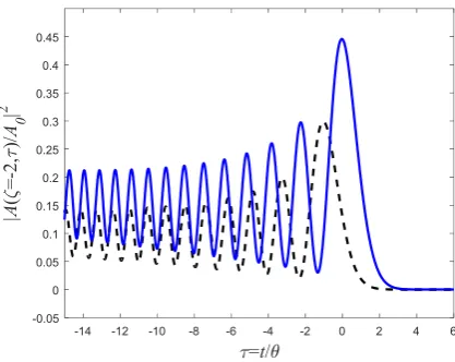
The profile of Eq.(14) is plotted in Fig.1 and a spatiotemporal presentation of its intensity A
( )
t,z 2 is presented139
θ ≡
τ t/ and 2
2 /θ β ≡
ζ z .
141
-10 -8 -6 -4 -2 0 2 4 6 8 10
-0.5 0 0.5 1
A
(
=2,
)/
A 0
-10 -8 -6 -4 -2 0 2 4 6 8 10
=t/ -0.4
-0.2 0 0.2 0.4
A
(
=2,
)/
A 0
142
Fig.1: The real (upper panel) and imaginary (lower panel) components of the pulse (14). The dashed curve
143
represents the initial profile (for / 2 0
2 θ =
β =
ζ z ), while the solid curve represents the signal after a distance,
144
which corresponds to / 2 2
2 θ =
β =
ζ z . Time is measured in units of θ, which corresponds to the pulse's
145
temporal width.
146
147
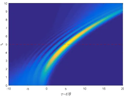
Fig.2: A false-color presentation of the pulse's intensity A
( )
t,z 2(Eq.(14)) as a function of the normalized time148
θ ≡
τ t/ and the normalized distance 2
2 /θ
β ≡
ζ z .
149
150
Sample Application: The pulses that many mode locked lasers emit can be simulated by Gaussian pulses (see
151
carrier wavelength of λ=1.06μm enters a BK7 glass, then 24ps2/Km 2 ≅
β , and ζ=1 in Fig. 2
153
corresponds to z / 2 30m 2
≅ β ζθ
= .
154
155
4.2 Boosted Gaussian
156
When the initial pulse is a boosted Gaussian
157
(
t z)
A(
t i t)
A 0
2 2 0exp / 0
, = = − θ + ω (15)
158
then using relation (6), the final profile is
159
( )
(
)
β − θ
ω β + −
β ω + ω β
− θ
θ =
z i
z t t
i z i z i A z
t A
2 2
2 0 2 0
2 0 2 2
2 0
2 exp
2 exp 2
, (16)
160
which means that beside the pulse spreading, the pulse's peak propagates with reciprocal "velocity" β2ω0. The
161
larger the spectral shift ω0 the larger is the temporal shift of the pulse. The pulse's profile and its intensity's
162
dynamics are presented in Figs.3 and 4 respectively.
163
164
Fig.3: The real (upper panel) and imaginary (lower panel) components of the Gaussian pulse (16). The dashed
165
curve represents the initial profile (for / 2 0
2 θ =
β =
ζ z ), while the solid curve represents its final shape (for
166
2 / 2
2 θ =
β =
168
Fig.4: Same as Fig.2 but for the intensity ( A
( )
t,z 2) of the pulse presented by Eq.(16)169
(in this example ω0=−4/θ).
170
4.3 Chirped Gaussian
171
When the initial pulse is chirped, i.e., the pulse's phase has an additional quadratic dependence on time, i.e.,
172
( )
− θ −
= 2
2 2
0exp
0
, A t iqt
t
A (17)
173
then, using Eq.(10) the final pulse is
174
( )
(
)
(
)
θ − β +
+ θ θ
− θ − β +
= −2
2 2
2 2
2 2
0
2 1
1 exp
/ 2
1 ,
i q z iq t
i q z A z
t
A (18)
175
In Fig. 18 the temporal dynamics of the pulse (18) is presented for the same parameters as Fig.2 but with
176
additional 2/ 2 θ − =
q . The shrinkage of the pulse's width is clearly shown, which is a consequence of the fact
177
that the chirping has widened the spectral width of the initial pulse.
178
-4 -3 -2 -1 0 1 2 3 4
=t/
0 0.1 0.2 0.3 0.4 0.5 0.6 0.7 0.8 0.9 1
179
Fig.5 Same as Fig.2 but for the intensity ( A
( )
t,z 2) of the pulse presented by Eq.(18) (in this example180
2 / 2 θ − =
q ).
5. Singular Pulses
182
Before going into the propagation of profiles, which can simulate real pulses, it is instructive to investigate a
183
family of pulses with singularity points. The singularity points are points, in which either the pulse's amplitude
184
or its derivatives are discontinuous. Despite their singularities, these pulses can simulate pulses, which have
185
sharp boundaries. Moreover, it will be shown that these generalized, i.e., singular, pulses can be modified very
186
simply into smooth ones, and therefore can be implemented in real, physical scenarios.
187
188
5.1 The Step Function
189
The step function response of a dispersive medium is related to the complex error function.
190
Let the initial pulse's profile be a step function, i.e.,
191
(
z t)
Au( )
tA =0, = 0 − (19)
192
where
( )
≤ > =
0 0
0 1
t t t
u is the Heaviside step-function, then, the pulse at the end of the medium is
193
( )
(
)
( )
β − =
β − − β
π −
=
∞ −
−
z i t erfc A dt z t t i z
i A
z t A
2 0
0
2 2 2
/ 1 2 0
2 2
1 ' 2
' exp
2
, . (20)
194
Clearly, if initially
195
(
z t)
Au(
t T)
A =0, = 0 − + (21)
196
then
197
( )
β −
− =
z i
T t erfc A z t A
2 0
2 2
1
, . (22)
198
Similarly, using (6) the initial boosted step function pulse
199
(
t z)
A( ) (
i tu t T)
A , =0 = 0exp ω0 − + (23)
200
will propagates to read
201
(
)
β −
ω β + −
ω + ω β =
>
z i
z T
t erfc t i z i A z
t A
2 0 2 0
2 0 2 0
2 2
exp 2 1 0
, . (24)
202
This result is known in the literature as Moshinsky's function. In Quantum Mechanics, this function was used to
203
simulate an electrons' beam, which was blocked by a beam shutter[19,20]. In the Quantum analogy, the
204
wavefunction exhibits interference in time.
205
206
5.2 Rectangular Pulses
207
The fundamental generalized pulse is the rectangular one. Unlike the delta function, the rectangular pulse has a
208
finite energy, and therefore can simulate in many scenarios, despite its singular edges, a real rectangular pulse,
209
The rectangular pulse can be written with the aid of the step function or the rectangular function
211
(
z=0,t)
=A0rect1( )
t/θ =A0[
u(
−t/θ+0.5) (
−u−t/θ−0.5)
]
A (25)
212
where
213
( )
> τ
≤ τ ≡ τ
2 / 0
2 / 1
rect
L L
L . (26)
214
Eq.(25) has two singular points (t=±0.5θ), in which the pulse's amplitude is discontinuous.
215
The dynamics of this rectangular pulse can be formulated analytically
216
( )
β −
θ + −
β −
θ − =
z i t erfc z i t erfc A z t A
2 2
0
2 2 / 2
2 / 2
1
, . (27)
217
In Fig.6 the real and imaginary components of (27) are plotted for two different medium's length. The ripples in
218
the pulse's profile appear after a very short distance.
219
220
A
(
=0.3,
)/
A 0
A
(
=0.3,
)/
A0
A
(
=0
.01,
)/
A 0
A
(
=0
.01,
)/
A 0
221
Fig.6: The real (upper panel) and imaginary (lower panel) components of the rectangular pulse (27). The dashed
222
curve represents the initial profile (for / 2 0
2 θ =
β =
ζ z ), while the solid curve represents its final shape (for
223
01 . 0 / 2
2 θ =
β =
ζ z on the right and / 2 0.3
2 θ =
β =
ζ z on the left).
224
225
227
Fig.7: Same as Fig.2 but for the intensity ( A
( )
t,z 2) of the pulse presented by Eq.(27)228
229
The intricate structure of this function is most pronounced when the incident signal is a train of rectangular
230
pulses
231
(
)
∞(
)
−∞ =
− θ =
=
n
n t rect A
t z
A 0, 0 1 / 2 . (28)
232
This case is equivalent to the well-known quantum problem of a particle in a 1D box, when initially the
233
particle's probability density is uniform over the box [21].
234
In this case the problem's dynamics can be formulated [using (27)] by
235
( )
∞−∞
=
β −
θ + − −
β −
θ − − =
n i z
n t erfc z
i n t erfc A
z t A
2 2
0
2 2 / 2 2
2 / 2 2
1
, . (29)
236
However, it should be emphasized, that in Ref.[21] a different numerical approach was taken, in which no error
237
function analysis was used.
238
239
Sample Application: In 10Gb/s optical communications channel (over smf28 fiber) with a carrier wavelength of
240
m
μ =
λ 1.55 , the pulses can be simulated by rectangular ones with θ=100ps and 20ps2/Km
2 ≅
β , in which
241
case ζ=0.3 in Fig.7 corresponds to z=ζθ2/β2≅150Km. However, as Fig.6 illustrates, considerable
242
distortions appear even for ζ=0.01, which corresponds to a fiber length of z≅5Km.
243
244
5.3 Chirped Rectangular Pulses
245
One of the methods to combat dispersion in optical communication is to chirp the pulses, and since most pulses
246
in optical communications are rectangular (in fact they are smooth rectangular, see below) it is instructive to
247
The initial chirped rectangular pulse has the following form
249
( )
0, exp(
)
( )
/ exp(
2)
[
(
/ 0.5) (
/ 0.5)
]
0 1
2
0 − θ = − − θ+ − − θ−
=A iqt rect t A iqt u t u t t
A . (30)
250
Therefore, using (10) and (24), the pulse profile after a distance z is
251
(
)
(
)
(
)
(
(
)
)
β + β −
β + θ + −
β + β −
β + θ − β
+
+ β
− = >
zq z
i
zq t
erfc zq z
i
zq t
erfc zq A zq
iqt t
z A
2 2
2
2 2
2
2 0
2 2
2 1 2
2 / 2 1 2
1 2
2 / 2 1 2
1 2 1 2 exp ,
0 (31)
252
Besides the widening of the pulse's boundaries, the boundaries also moves at a constant "velocity", i.e., the two
253
boundaries obey the following relationship
254
(
qz)
tB 1 2 2 2 + β θ ±
= (32)
255
Clearly, when q is positive, the two boundaries collide at a distance
256
q
zf =−1/2β2 , (33)
257
which is independent of the pulse's width θ. In Fig. 8 the propagation of this pulse for both positive and
258
negative q is presented.
259
-2 -1.5 -1 -0.5 0 0.5 1 1.5 2
=t/
0 0.05 0.1 0.15 0.2 0.25
260
Fig.8: Same as Fig.2 but for the intensity (A
( )
t,z 2) of the pulse presented by Eq.(31). On the left q=4/θ2,261
and on the right q=−4/θ2. The dashed lines corresponds to the pulse's boundaries t
(
1 2 2qz)
/2B=±θ + β .
262
263
While the pulse indeed shrinks for negative q, the pulse's minimum width is reached before the distance zf ,
264
i.e. Eq.(33). However, if the two pulses are combined, i.e., if the initial pulse is
265
(
0,)
cos( )
( )
/ cos( )
2[
(
/ 0.5) (
/ 0.5)
]
0 1
2
0 θ = − θ+ − − θ−
=
= t A qt rect t A qt u t u t
z
A (34)
then the minimum width occurs exactly at the distance zf. In Fig. 9 the temporal dynamics of this pulse is
267
presented, and the point zf is clearly shown. Clearly, a smoother, i.e., more realistic, pulse will not converge
268
to an infinitely temporally narrow pulse, but instead will converge to a finite temporal width.
269
270
Fig.9: Same as Fig.8 but with the initial pulse Eq.(34) for the parameter 4/ 2 θ =
q .
271
5.4 Exponential Pulse
272
The product of the step function with the exponential function allows investigating the dynamics of the simplest
273
exponential function. Utilizing (8), the initial exponential-step function
274
(
t,z 0)
A0exp( ) ( )
at At,0A = = (35)
275
will propagate in dispersive medium according to
276
(
)
β −
β −
− β + =
>
z i
az i t erfc at z a i A
t z A
2 2 2
2 0
2 2
exp 2 ,
0 . (36)
277
In Fig.10 the dynamics of the exponential-step function pulse is plotted.
278
279
A spatiotemporal presentation of the pulse's intensity is presented in Fig.11. This pulse can simulate a pulse
280
where its rise time is considerably shorter than its decay time. In both figures a=1/θ.
281
283
Fig.10: The real (upper panel) and imaginary (lower panel) components of the exponential-step function pulse
284
(36). The dashed curve represents the initial profile (for / 2 0
2 θ =
β =
ζ z ), while the solid curve represents its
285
final shape (for / 2 0.01
2 θ =
β =
ζ z ).
286
287
Fig.11: Same as Fig.2 but for the intensity (A
( )
t,z 2) of the pulse presented by Eq.(36).288
289
5.5 Cosine Pulse
290
A bounded cosine pulse is an example of a continuous pulse (unlike the rectangular one), where the
291
discontinuity at the edges of the pulse occurs on the amplitude's derivative level.
292
It should be stressed that in terms of the pulse's intensity, the derivative is continuous as well. Therefore, this is
293
an important pulse, because for many practical purposes, it mimics a continuous pulse, but at the same time, it is
294
(initially) temporally bounded.
295
In this case, if the initial pulse is
296
(
)
(
)
θ ≥
θ < θ π =
=0, cos0 / //22 t t t A t z
A , (37)
which can be rewritten as
298
(
)
(
)
(
)
θ − − θ π − + θ π − θ + − θ π − + θ π == exp exp /2 exp exp /2
2 ,
0t A i t i t u t i t i t u t
z
A , (38)
299
then, using (24) the pulse profile at the medium's end is
300
( )
β − πβ − + − π − β − πβ + + π − β − πβ − − − π + β − πβ + − π π β = z i T z T t erfc T t i z i T z T t erfc T t i z i T z T t erfc T t i z i T z T t erfc T t i T z i A t z A 2 2 2 2 2 2 2 2 2 2 0 2 / 2 / exp 2 / 2 / exp 2 / 2 / exp 2 / 2 / exp 2 exp 4 ,301
(39)302
Fig.12 illustrates the dynamics of the pulse presented by Eq.(39).
303
304
Fig.12: Similar to Fig.10 but for the bounded cosine pulse [Eq.(39)], and for the final distance of
305
3 . 0 / 2
2 θ =
β =
ζ z .
306
A spatiotemporal presentation of the pulse's intensity is presented in Fig.13.
307
-2 -1.5 -1 -0.5 0 0.5 1 1.5 2
=t/
0 0.05 0.1 0.15 0.2 0.25 0.3
308
310
5.6 Square Cosine Pulse
311
A smoother pulse profile is the square cosine one. In this case, the discontinuity occurs in the second derivative
312
level, but the function itself and its derivative are both continuous. Therefore, this pulse can simulate pulses,
313
which were generated by discontinuous dielectric media. Let
314
(
)
(
)
θ ≥ θ < θ π = = 2 / 0 2 / / cos , 0 2 0 t t t A t zA (40)
315
be the signal's profile at one end of the medium, then, since it can be rewritten as
316
(
)
exp 2 exp 2 2[
(
/2) (
/2)
]
4 1 ,
0 0 − +θ − − −θ
+ θ π − + θ π =
= t A i t i t u t u t
z
A (41)
317
Its dynamics can be derived, again using (24), to yield the result
318
319
( )
β − πβ − + − π − β − πβ + + π − β − πβ − − − π + β − πβ + − π π β β − + − β − − = z i T z T t erfc T t i z i T z T t erfc T t i z i T z T t erfc T t i z i T z T t erfc T t i T z i z i T t erfc z i T t erfc A z t A 2 2 2 2 2 2 2 2 2 2 2 2 0 2 / 2 / exp 2 / 2 / exp 2 / 2 2 / 2 exp 2 / 2 2 / 2 exp 2 2 exp 2 2 / 2 2 / 4 1 ,320
(42)321
Fig.14 presents the dynamics of the square cosine pulse.
322
A ( =0 .3 , )/ A 0 A ( =0 .3 , )/ A 0323
Fig.14: Similar to Fig.12 but for the square cosine pulse[Eq.(42)].
324
A comparison between (27), (39) and (42) is presented in Fig.15. The three pulses represents three levels of
326
singularities. Eq.(27) represents a case of amplitude discontinuity, Eq.(39) represents discontinuity in the
327
pulse's amplitude's derivative, and Eq.(42) represents discontinuity in the amplitude's second derivative.
328
As can clearly be seen, the higher is the level of the singularity (i.e., the discontinuity occurs at higher
329
derivatives) the faster the pulse decays in accordance with Refs.[22] and [23].
330
0 1 2 3 4 5 6 7 8 9 10
=t/
10-10 10-8 10-6 10-4 10-2 100
|
A
(
=0.
1,
)/
A 0
|
2
rect cos rect cos2 rect
331
Fig.15: Comparison between the intensities of the three singular pulses Eq.(27)- dashed curve, Eq.(39)-solid
332
curve, and Eq.(42)-dotted curve in a logarithmic scale.
333
334
5.7 Generalization and Applicable Examples
335
The mathematical tools that were presented in the previous sections can be implemented in numerous practical
336
examples. In what follows we will present some examples.
337
338
1st example:
339
Generalization to any power of the bounded cosine pulse, i.e.
340
(
)
(
)
≥ < π
= =
2 / 0
2 / /
cos ,
0 0
T t
T t T t A
t z A
n
for any n (43)
341
which can be written as
342
(
)
exp exp[
(
/2) (
/2)
]
2 1 ,
0 0 t u t T u t T
T i t
T i A t
z A
n
n − + − − −
− π
+
π
=
= (44)
343
and since the brackets can be expanded
344
(
)
exp(
2)
[
(
/2) (
/2)
]
2 1 , 0
0
0 t u t T u t T
T n k i k n A t
z A
n
k
n − + − − −
− π
=
=
=
(45)
345
(
)
(
)
(
)
(
)
(
)
β − πβ − − − π − − − β − πβ − + − − π × π β × = =
= z i T z n k T t erfc T t n k i z i T z n k T t erfc T t n k i T z i k n A t z A n k n 2 2 2 2 0 2 2 0 2 / 2 2 2 / 2 exp 2 / 2 2 / 2 exp 2 2 exp 2 1 , 0 (46)347
2nd example:348
The initial singular pulse
349
(
z t)
A( )
atA =0, = 0exp− (47)
350
consists of two exponential pulses, and therefore its propagation can be expressed in a relatively simple form,
351
namely352
(
)
( )
( )
β − β − − − + β − β − − β = > z i az i t erfc at z i az i t erfc at z a i A t z A 2 2 2 2 2 2 0 2 exp 2 exp 2 exp 2 ,0 . (48)
353
3rd example:
354
355
In the previous example, we sew two singular pulses; in general, however, one can sew several pulses together
356
to create a combined pulse, which is much smoother than its singular components. For example, take the
357
following pulse profile
358
(
)
(
)
[
(
( )
)
(
)
]
≥ − − < = = 2 / 2 / tan 2 / exp 2 / cos 2 / cos , 0 0 0 T t kT T t k kT A T t kt A t zA (49)
359
which consist of three singular and discontinuous pulses; however, the combined pulse and its derivative are
360
4th example:
364
365
The discontinuity of the exponential pulse can be reduced by multiplying the pulse by a sine function, i.e.,
366
(
z t)
A( ) ( ) ( )
at btu tA =0, =− 0exp sin − . (51)
367
Since the pulse can be written as
368
(
z t)
iA[
(
(
a ib)
t)
(
(
a ib)
t)
]
u( )
tA = = exp + −exp − −
2 ,
0 0 (52)
369
then the pulse's amplitude after a distance z reads
370
( )
(
)
(
)
(
)
(
)
(
)
β −
− β − −
β − −
β −
+ β − +
β
×
+ − β − =
z i
ib a z i t erfc ibt abz z
i ib a z i t erfc ibt abz
at z b a i iA
z t A
2 2 2
2 2 2
2 2 2 0
2 exp
2 exp
2 exp 4 ,
(53)
371
In Fig.16 this pulse is presented for two cases with different parameters. On the right figure the frequency is
372
equal to the decaying coefficient a, however, on the left one the frequency is higher than the decaying
373
exponent a, and therefore the profile initially oscillates.
374
375
376
Fig.16: Similar to Fig.10 but for the pulse presented by Eq.(53). In these plots, a=1/θ on both, but b=4/θ
377
on the left figure (final distance corresponds to / 2 0.1
2 θ =
β =
ζ z ) and b=1/θ on the right one (final distance
378
corresponds to / 2 0.2
2 θ =
β =
ζ z ).
379
380
6. Smooth Pulses
381
Thus far, we have analyzed, except for the Gaussian pulses, only singular pulses, i.e., pulses' profiles, which
382
have at least one singularity point. Most of them can simulate real physical pulses' profiles; however, one may
383
argue that these pulses fundamentally cannot behave like physical pulses. In some respects, it is indeed a
384
justified claim, especially for short medium. It has been shown that since the dispersion equation is not a causal
385
comes out that there is a very elegant method, to convert each one of these singular pulses to a smooth one,
387
which can simulate, in all respect, a real physical profile pulse. This method was first presented in Refs. [23] and
388
[24] for the rectangular pulse.
389
390
6.1 Smooth Step Function
391
In principle, any smooth step function can replace the Heaviside step function, however, there is a clear
392
advantage to choose the complementary error function for that purpose. The function
393
Δ t erfc 2 1
(54)
394
is an approximation of the step function in the sense that
395
( )
tu t erfc
t = −
Δ →∞
Δ 2
1 lim
/ (55)
396
However, unlike the step function, the transition in (54) occurs within the time scale Δ.
397
Equivalently, a step function signal that passes through a Gaussian low-pass filter, whose spectral FWHM is δ
398
will have the following form [11]
399
πδ 2 ln 2 2
1 t
erfc . (56)
400
Therefore, the relation between the transition time scale Δ and the spectral FWHM δ is
401
( )
θ πΔ=
δ 2ln2 / . (57)
402
Moreover, and this is the reason that (54) is very useful in replacing step functions, the smooth step (54) can be
403
written as a convolution between the step function and a Gaussian, i.e.
404
( )
( )
(
)
( )
(
2 2)
2 2 /
2
/ exp 1 *
/ exp 1
exp 1 2
1
Δ − π Δ −
= τ Δ τ − − τ π Δ = − π
=
Δ
∞
∞ − ∞
Δ
t t
u
d t
u dx
x t
erfc
t (58)
405
where the asterisk represents temporal convolution. However, since the effect of dispersion can also be
406
represented as a convolution with the kernel (4), then the propagation of the initial pulse' profile
407
( )
Δ = A erfc t t
A
2 0
, 0 (59)
408
can be written simply as
409
( )
( )
(
)
( )
β − Δ =
Δ − π Δ − =
z i t erfc A z t K t
t u A t A
2 2 0
2 2 0
2 2
1 , * / exp 1 * 0
, (60)
410
Therefore, every step function from the previous section can be replaced with the smooth step function. In
411
(
)
(
)
Δ ω − == t A i t erfc t
z
A exp 0
2 ,
0 (61)
413
will have the following profile at the end of the medium
414
(
)
β − Δ ω β − β ω − ω = > z i z t erfc t i z i A t z A 2 2 0 2 0 2 0 2 2 2 exp 2 ,0 (62)
415
Sample Applications: The rise time of pulses in optical communications are usually defined as the time-period it
416
takes to rise from 10% to 90% maximum intensity value. Therefore, provided this rise-time (Δt10−90) is given
417
then Δ can be derived by Δ≅0.67Δt10−90. If the rise time is defined as the period, in which the signal rises
418
from 25% to 75% of its maximum intensity value (Δt25−75), then Δ≅1.28Δt25−75.
419
420
6.2 Smooth Rectangular Pulse
421
Similarly, the smooth rectangular pulse
422
(
)
Δ θ + − Δ θ − == /2 /2
2 ,
0t A0 erfc t erfc t z
A (63)
423
will appear at the end of the medium in the following form
424
(
)
( )
Δ + β − θ + − Δ + β − θ − = θ β Δ π θ θ = > 2 2 2 2 0 2 2 1 0 2 2 / 2 2 / 2 , 2 ln 2 , srect , 0 z i t erfc z i t erfc A z t A t z A (64)425
where426
(
)
(
)
( )
(
/2)
/ 2 2ln( )
2 / /2erfc / 2 ln 2 2 / 2 / erfc , , srect 2 2 2 2 τ+ξ ζ+ π δ − τ−ξ ζ+ π δ ≡ ζ δ τ ξ i i (65)
427
is the smooth rectangular function (see Refs.[23-25]), which describes the dispersion dynamics of a smooth
428
rectangular pulse.
429
In Fig. 17 this smooth rectangular pulse's profile is presented for the same values as in Fig.6, i.e. the perfect
430
rectangular pulse. However, the difference is that in Fig.17 the pulse's boundaries are smooth instead of
431
discontinuous. As can be seen, due to the smooth transition, the oscillations, which appear in Fig.6 disappear in
432
434
Fig.17: Same as Fig.12, but for Eq.(64) with the transition width Δ=0.2θ
435
436
This pulse has numerous applications in optical communications.
437
For example, if the transmitted data is encoded in the amplitudes of these smooth rectangular pulses, then the
438
transmitted signal profile can be written
439
(
)
( )
θ β Δ π
θ −
θ =
> ξ
n
n t n z
a z
t
A 2
2 / , 2 ln 2 , / srect 0
, . (66)
440
where an are coefficient, which carry the data.
441
These pulses has two properties that make them especially suitable for stream of pulses.
442
The ξ parameter can determine the signal's protocol. The Return-to-Zero (RZ) protocol occurs for ξ<1,
443
when ξ determines the duty cycle. However, when ξ=1 then this is a perfect Non-Return-to-Zero (NRZ)
444
protocol. The second property, which is more important, emerges due to symmetry of the erfc function. Since
445
2 =
Δ − +
Δ
t erfc t
erfc (67)
446
then two adjacent smooth rectangular pulses look exactly like a single but twice as wide a pulse, i.e.
447
(
τ−0.5,δ,ζ)
+srect(
τ+0.5,δ,ζ)
=srect(
τ,δ,ζ)
srect1 1 2 (68)
448
449
Sample Application: In 40Gb/s optical communications channel (over smf28 fiber) with a carrier wavelength of
450
m
μ =
λ 1.55 , the pulses can be simulated by rectangular ones with θ=25ps, 20ps2/Km
2 ≅
β , in which case
451
3 . 0 =
ζ and ζ=0.01in Fig.17 correspond to z / 2 9.4Km 2
≅ β ζθ
= , and z≅0.31Km respectively. Since
452
θ =
Δ 0.2 then the 10%-90% rise time correspond to Δt10−90≅Δ/0.67=0.2θ/0.67≅7.5ps.
453
454
6.3 Relations to Super-Gaussian Pulses
455
(
z t)
A[
( )
t T n]
A =0, = 0exp− / (69)
457
be a super-Gaussian pulse. This pulse can be approximated by a smooth rectangular one (Eq.(63)]
458
(
z=0,t)
=A0[
erfc(
(
t−θ/2)
/Δ)
−erfc(
(
t+θ/2)
/Δ)
]
/2A by choosing the following parameters
459
( )
nT 1/ 2 ln 2 =
θ (70)
460
and
461
( )
( )n nn T
/ 1
2 ln
2 −
π =
Δ (71)
462
A
(
=0,
)/
A 0
-3 -2 -1 0 1 2 3
=t/
0 0.1 0.2 0.3 0.4 0.5 0.6 0.7 0.8 0.9 1
A
(
=0
,
)/
A0
n=4
463
Fig.18: A comparison between smooth rectangular pulses Eq.(63) (solid curves) and super-gaussian pulses
464
Eq.(69) (dashed curves) for n=4 (right) and n=14 (left). In these plots only the real part of the fields is
465
presented. The imaginary part is zero.
466
467
In Fig.18 such a comparison is presented for two different values of the super Gaussian order n. This figure
468
clearly shows that the smooth rectangular is an excellent approximation to super-Gaussian, while unlike
469
super-Gaussian, the smooth rectangular pulse does have an exact analytical expression for its propagation in
470
dispersive medium.
471
472
6.4 Chirped Smooth Rectangular Pulse
473
The case of the chirped rectangular pulse can be generalized to the chirped smooth rectangular one. That is, if
474
the initial pulse's profile is
475
(
)
( )
Δ θ + −
Δ θ − −
=
= exp /2 /2
2 ,
0t A0 iq2t erfc t erfc t z
A (72)
476
(
)
(
)
Δ + β + β − θ + β + − Δ + β + β − θ − β + + β − β + = > − 2 2 2 2 2 2 2 2 0 2 2 2 / 1 2 2 1 2 2 / 2 1 2 1 2 2 / 2 1 2 / 1 2 exp 2 1 , 0 zq z i zq t erfc zq z i zq t erfc A q z t i zq t z A478
(73)479
A spatiotemporal presentation of the pulse's intensity is presented in Fig.18. The fact that the initial pulse is
480
smooth eliminates the ripples that appear in Fig.9.
481
-2 -1.5 -1 -0.5 0 0.5 1 1.5 2
=t/
0 0.05 0.1 0.15 0.2 0.25
-2 -1.5 -1 -0.5 0 0.5 1 1.5 2
=t/
0 0.05 0.1 0.15 0.2 0.25
482
Fig.18: Same as Fig.8 but for a smooth rectangular pulse with Δ=0.25θ.
483
484
6.5 Smooth Cosine Pulse
485
As was said above, the same procedure can be applied to every singular pulse, i.e., to replace the singular step
486
function with the erfc functions. For example, the singular cosine pulse (37) can be replaced with the following
487
smooth cosine one
488
(
)
Δ θ + − Δ θ − θ π ==0, 0cos /2 /2
t erfc t erfc t A t z
A (74)
489
which has the following solution for any distance z:
490
( )
β − Δ θ πβ − θ + θ π − − β − Δ θ πβ + θ + θ π − β − Δ θ πβ − θ − θ π − + β − Δ θ πβ + θ − θ π θ π β = z i z t erfc t i z i z t erfc t i z i z t erfc t i z i z t erfc t i z i A t z A 2 2 2 2 2 2 2 2 2 2 2 2 2 2 0 2 / 2 / exp 2 / 2 / exp 2 / 2 / exp 2 / 2 / exp 2 exp 4 ,491
(75)492
494
Fig.19: Same as Fig.12, but for Eq.(75) with the transition width Δ=0.4θ
495
Clearly, the same procedure can be implemented on the square cosine pulse or on any other singular pulse from
496
the previous sections.
497
498
6.6 Smooth Exponential Pulse
499
By following the same procedure, one can replace the singular exponential with the following smooth
500
exponential pulse
501
(
)
( )
Δ =
= t A aterfc t
z
A exp
2 1 ,
0 0 (76)
502
which propagates in dispersive medium according to
503
(
)
β − Δ
β −
− β +
= >
z i
az i t erfc at z a i A
t z A
2 2
2 2
2 0
2 2
exp 2 ,
0 (77)
504
This function is illustrated in Fig.20 for two different distances.
505
506
Fig.20: Same as Fig.10, but for Eq.(77) with the transition width a=1/θ and Δ=0.2θ, for two final
507
distances / 2 0.01
2 θ =
β =
ζ z on the left and / 2 0.1
2 θ =
β =
509
Sample Application: A pulse with a 10% to 90% rise time of Δt10−90=1ps and a decay time of ~3.7ps
510
with a carrier wavelength of λ=2.0μm, can be simulated by the pulse presented by Eq.(76) with
511
ps
67 . 0
=
Δ , a=0.3ps−1 . Since aΔ≅0.2, Fig.20 is an illustration of this pulse. If the pulse penetrates
512
a BK7 glass then for this wavelength 98ps2/Km
2 ≅
β , and therefore ζ=0.1 and ζ=0.01in the
513
figure correspond to z / 2 11m 2 β ≅ ζθ
= , and z≅1.1m respectively.
514
515
7. Singular Pulses in the Spectral Domain
516
7.1 The ideal Nyquist Sinc Pulse
517
One of the interesting and important pulses, which belongs to this category and received a lot of attention
518
recently in the literature, is the Nyquist-Sinc pulse (see, for example, Refs.[26-31]).
519
These pulses are useful in optical communications for several reasons, one of which is that they are resilient
520
against chromatic dispersion. Moreover, these pulses, like their Fourier counterpart – the rectangular pulses, are
521
orthogonal both in the time and in the frequency domains.
522
The initial Nyquist-Sinc pulse is singular in the spectral domain, i.e. its Fourier transform is
523
(
z=0,ω)
=θA0rect1(
ωθ/2π)
A . (78)
524
In the temporal regime the "sinc" profile appears
525
(
)
≡ π(
πθθ)
θ =
=
/ / sin sinc
,
0 0 0
t t A t A t z
A . (79)
526
Since the pulse's spectrum has a simple rectangular shape, the temporal dynamics is straightforward, namely
527
( )
( )
β θ πβ + − −
β θ πβ − −
β − πβ
θ
≡ ζ τ =
z i
z t z
i z t z
t i z i A
A t z A
2 2
2 2
2 2
2 2 0
0
2 / erf
2 / erf
2 exp 2
2
, dsinc ,
(80)
528
where
529
( )
ζ ζ π + τ − −
ζ ζ π − τ −
ζ τ − πζ ≡ ζ τ
2 erf 2 erf 2 exp 2 2 1 , dsinc
2
i i
i
i (81)
530
is the "dynamic" sinc function[12]. Clearly
(
)
( )
( )
πτ πτ ≡ τ = = ζ
τ, 0 sinc sin
dsinc .
531
533
Fig.21: Same as Fig.10, but for Eq.(80) and for the final distance of / 2 0.3
2 θ =
β =
ζ z
534
535
The spatiotemporal presentation of the pulse's intensity is presented in Fig.22.
536
537
Fig.22: Same as Fig.2 but for the intensity (A
( )
t,z 2) of the pulse presented by Eq.(80).538
539
7.2 Nyquist Sinc Pulse with Smooth Spectrum
540
Singular spectrum may simulate real pulses, but in real scenarios, singularities can neither occur in the spectral
541
domain. We can therefore utilize the theorems and conclusions from the previous sections to smooth spectrally
542
the Nyquist-Sinc pulse.
543
Thus, the singular rectangular spectrum of the Nyquist-Sinc pulse, i.e.,
544
(
z=0,ω)
=θA0rect1(
ωθ/2π)
A (82)
545
can be replaced with its smooth counterpart
546
(
)
Δ θ π + ω −
Δ θ π − ω θ
= ω
=0, A012 erfc / erfc /
z
A . (83)