Magnetic Quantum Otto Engine for the
Single-Particle Landau Problem
Francisco J. Peña1*, A. González1, A. S. Nunez2, P. A. Orellana1, René G. Rojas3and P. Vargas1 1 Departamento de Física, Universidad Técnica Federico Santa María Casilla 110 V, Valparaíso, Chile ;
2 Departamento de Física, Facultad de Ciencias Físicas y Matemáticas, Universidad de Chile, Casilla 487-3,
Santiago, Chile; [email protected]
3 Instituto de Física, Pontificia Universidad Católica de Valparaíso, Av. Brasil 2950, Valparaíso, Chile; [email protected]
* Correspondence: [email protected]
Abstract:We study the effect of the degeneracy factor in the energy levels of the well-known Landau problem for a magnetic quantum Otto engine. The scheme of the cycle is composed of two quantum adiabatic processes and two quantum isomagnetic processes driven by a quasi-static modulation of external magnetic field intensity. We derive the analytical expression of the relation between the magnetic field and temperature along the adiabatic process and, in particular, reproduce the expression for the efficiency as a function of the compression ratio.
Keywords:quantum thermodynamics; degeneracy effects ; magnetic quantum engine.
1. Introduction
Quantum thermodynamics is one of the most interesting topics in physics today. The possibility to create an alternative and efficient nanoscale device, like its macroscopic counterpart, introduces the concept of the quantum engine, which was proposed by Scovil and Schultz-Dubois in the 1950’s [1]. The key point here is the quantum nature of the working substance and of course the quantum versions of the laws of thermodynamics [2–18]. The combination of these two simple facts leads to very interesting studies of well-known macroscopic engines of thermodynamics, such as Carnot, Stirling and Otto, among others [2–4]. The maximum efficiency of these engines is governed by the Carnot efficiency, and this cannot be surpassed unless the reservoirs are also of a quantum nature, for example, modeled as quantum coherent states or squeezed thermal states [4–6].
The classical Otto engine consists of two isochoric processes and two adiabatic processes. If the working substance is a classical ideal gas, the first approximation for efficiency depends on the quotient of the temperatures in the first adiabatic compression [19,20]. This expression is reduced with the specific condition along the adiabatic trajectory for this kind of gas, given byTVγ−1=cnt., where γ=CP/CVobtaining the expressionη=1− rγ1−1, whereris defined as a “compression ratio" that is defined asV1/V2(withV1>V2) [19]. On the other hand, the quantum Otto engine consists of two quantum adiabatic processes, which keeps invariant the probability occupation for the level of energy, and two quantum isochoric processes, in order to keep constant some parameters in the Hamiltonian. In this context, the quantum harmonic Otto cycle is a hot research topic, fully addressed by Kosloff and Rezek [21], and with a recent experimental realization employing a single ion in harmonic trap [22]. In the magnetic scenario, it is useful to think that the “isochoric process” is replaced by “isomagnetic ” ones [12,13]. Therefore, the constant value in the process corresponds to the value of cyclotron frequency (or effective frequency depending on the case), which is proportional to the intensity of the magnetic field. This kind of approach is developed in the Ref. [13], for the case of a graphene under strain and the presence of the external magnetic field, exhibiting that the Carnot efficiency is achieved more quickly with the combination of these two effects as opposed to only applying strain to the sample.
The Landau levels of energy in condensed matter physics constitutes a very well-known case and a typical academic problem. The thermodynamics is fully addressed in the works of Kumar et al. [23] and one important point is the degeneracy factor present in the partition function, and consequently also present in the entropy. So, if we consider a thermodynamic cycle, where it is proposed to control the magnetic field along the adiabatic trajectories, it leads to very interesting new results and can be contrasted with the harmonic case. In this same framework, we highlight the work of Mehta and Ramandeep [24], who worked on a quantum Otto engine in the presence of level degeneracy, finding an enhancement of work and efficiency for two-level particles with a degeneracy in the excited state. This work proposes to study the magnetic Otto cycle for the Landau problem and to understand the role of the degeneracy factor along the cycle. In particular, we found an analytical dependence between the magnetic field and temperature along the adiabatic process, and we use these results to calculate the efficiency of this cycle. We compare this efficiency with that corresponding to the harmonic trap with the same parametrization to see how strong the effect of this factor is on the results.
2. Partition Function for the Single-Particle Landau Problem
We consider the case for an electron with an effective massm∗and chargeeplaced in a magnetic field, where the Hamiltonian of this problem working in the symmetric gauge leads to the known expression
ˆ H= 1
2m∗ "
px−eBy 2
2 +
py+exB 2
#
, (1)
and the corresponding Landau levels display the energy spectrum
En =h¯ωB
n+1 2
, . (2)
Here,n=0, 1, 2,...is the quantum number, and
ωB= eB
m∗ (3)
is the standard definition for the cyclotron frequency [12,13,23]. With the definition of the parameter ωB, we can define the Landau radius that captures the effect of the intensity of the magnetic field, given bylB=
p ¯
h/(m∗ωB). The energy spectrum for each level is degenerate with a degeneracyg(B) given by [23]
g(B) = eB
2π¯hA, (4)
withAbeing the area of the box perpendicular to the magnetic fieldB. So, with this approach it is straightforward to calculate the partition function to Landau problem, and it turns out to be
Z= m
∗
ωBA 4π¯h csch
β¯hωB
2
, (5)
which corresponds to standard partition function for a harmonic oscillator in the canonical ensemble, with a degeneracy for level equal tog(B).
3. Quantum Thermodynamics and Magnetic Quantum Otto Engine
3.1. The First Law of Quantum Thermodynamics
derivate this law simply, consider a Hamiltonian with an explicit dependence of some parameter that we will callµin a generic form [25]. So, you have a set of eigenvectors of ˆHthat satisfy the eigenvalue problem
ˆ
H|n;µi=En|n;µi, (6)
wherenrepresents a set of indexes that label the spectrum of the Hamiltonian and|n;µiconstitutes the set of eigenvectors of ˆH. On the other hand, the density matrix is diagonal in the energy eigenbasis. Therefore, the ensemble-average energyE=hHˆiis reduced to
E=
∑
nPn(µ)En(µ), (7)
for a given occupation distribution with probabilitiesPn(µj)in thenth eigenstate.
The statistical ensemble just described can be submitted to an arbitrary quasi-static process, involving the modulation of the parameter µ, and hence the ensemble average energy changes accordingly,
dE =∑n(En(µ)dPn(µ) +Pn(µ)dEn(µ)) (8) =δQ+δW.
The last equation corresponds to the first law of quantum thermodynamics [2–18,21–26]. The first term in Eq.(8) is associated with the energy exchange, while the second term represents the work done. That is, the work performed corresponds to the change in the eigenenergiesEn(µ). It is in agreement with the fact that work can only be carried out through a change in generalized coordinates of the system, which in turn gives rise to a change in the eigenenergies [9,10].
The usual expression for the entropy is given by the von Neumann form in the eigenenergy base as
S(µ) =−kB
∑
nPn(µ)ln[Pn(µ)], (9)
where the coefficientsPn(µ)satisfy that 0≤Pn(µ)≤1 and the normalization condition
∑
n
Pn(µ) =1. (10)
3.2. Magnetic Quantum Otto Engine
As mentioned before, the result of the efficiency of the conventional Otto cycle can be written in the form that the results only depend on the quotient of the temperatures in the first adiabatic compression. By using the properties of the ideal gas, the efficiency can be rewritten as follows:
η=1− 1
rγ−1, (11)
whereγ=CP/CVis the quotient of the two specific heat (at constant pressure and at constant volume) andris know as “compression ratio" which is defined asV1
V2 (withV1>V2).
On the other hand, the quantum “conventional" Otto engine is composed of two quantum isochoric processes and two quantum adiabatic processes. For the first process mentioned, the occupation probabilitiesPn(µ)change and thus the entropySchanges, until the working substance finally reaches thermal equilibrium with the heat bath. For the case of the quantum adiabatic process, the population distributions remain unchanged, that isdPn(µ) =0. Thus, no transition occurs between levels, and no heat is exchanged during this process. It is important to recall that a classical adiabatic process does not necessarily require the occupation probabilities to be kept invariant [26].
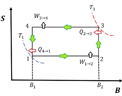
Figure 1.The magnetic quantum Otto engine represented as an entropy (S) versus a magnetic field (B) diagram.
value ofγfor that case. For the magnetic case, the two quantum isochoric trajectories are replaced by two “isomagnetic" ones, where the principal finding is the possibility to keep constant the value of the magnetic field intensity along the process while heat is exchanged between the system and the reservoirs [13].
Let us consider a cycle by devising a sequence of quasi-static trajectories, as depicted in Fig.1. First, the system, while submitted to an external magnetic fieldB1, is brought into thermal equilibrium with macroscopic thermostats at temperature T1. In equilibrium, the probabilitiesPn(µ) take the Boltzmann form and can work with a partition function in the canonical ensemble,Z(µ,T). So, the Helmholtz free energy can be defined byF(µ,T) =−kBTlnZ(µ,B)and the entropy given by Eq.(9) can be written asS(µ,T) = E(µT,T)+kBlnZ(µ,T), where the ensemble average energy is given by
E(µ,T) =kBT2 ∂
∂TlnZ(µ,T). (12) Here, theµparameter is related to the intensity of the magnetic field, soµ→Bfor the case under the study. Then, the system is submitted to a quantum isoentropic process from 1 →2, increasing the magnitude of the magnetic field fromB1toB2. The systems perform work along the isoentropic trajectory according to
W1→2= Z B2
B1 dB
∂E ∂B
Pn(B)=cnt. =
Z B2
B1 dB
∂E ∂B
S
=E(T2,B2)−E(T1,B1).
(13)
For the case of the “isomagnetic" heating process with the intensity of magnetic field equal toB2from 2→3, no work is done, but heat is absorbed. The heat absorbed (Q2→3) is given by the expression
Q2→3= Z T3
T2 dT
∂E ∂T
B2
=E(T3,B2)−E(T2,B2).
(14)
In the same way discussed before, the isoentropic trajectory from 3→4, the system performs work in the form
W3→4=E(T4,B1)−E(T3,B2). (15) A physical interpretation of the work performed by the engine is obtained by considering the statistical mechanical definition of the ensemble-average magnetization, M = −∂E
∂B
S. Hence, the works defined in Eqs. (13) and (15) can also be interpreted asW=−R
Similarly, we obtain the heat released to the low temperature sink in the quantum “isomagnetic" cooling process from 4→1
Q4→1= Z T1
T4 dT ∂E ∂T B1
=E(T1,B1)−E(T4,B1).
(16)
The efficiency of the engine is then given by the expression
η=
W1→2+W3→4 QH
=1−
E(T1,B1)−E(T4,B1) E(T3,B2)−E(T2,B2)
. (17)
If we have the analytic function for the entropy, the intermediate temperaturesT2andT4must be determined to reduce the expression for efficiency and can take on two different forms:
• Deducting the relation between the magnetic field and the temperature along an isoentropic trajectory solving the differential equation of first order given by
dS(B,T) = ∂S ∂B T dB+ ∂S ∂T B
dT =0, (18)
which can be written as
dB dT =−
CB T∂S∂B
T
, (19)
whereCBis the specific heat at constant magnetic field.
• The other possibility is connecting the value for the entropy in two isoentropic trajectories in the form
S(B1,T1) =S(B2,T2) S(B2,T3) =S(B1,T4),
(20)
finding the function for magnetic field in terms of the temperature through numerical calculation. Finally, we parametrize this dependency in the efficiency by defining the ratio
r= lB1 lB2
, (21)
which represents the analogy of the compression ratio for the classical case. It is important to remember that the Landau radius is inversely proportional to the magnitude of the magnetic field. Therefore, for a major (minor) magnitude of the field, the Landau radius is smaller (bigger), and theris well defined. It is important to highlight the work of Zheng and Poletti [27], where they derived a general form for the efficiency of quantum Otto cycles with power law trapping potentials, corresponding to Eq. (11), and showed thatγmust be equal to three. We remark that this result requires that two conditions be met. First, it is only valid for the non-degenerate cases, or more specifically, when the degeneracy is independent of the parameter that rules the cycle. The second condition is that the expansion process, when the system goes toω0→ω00, must follow the following relation
κ≡ En(ω
0)
En(ω00) =
ω0
ω00 α
, (22)
whereαdepends on the power of the potentials under study. For example, for a conventional harmonic trap, the spectrum of energy is alwaysEn=h¯ω
The case of the Landau problem is different. The energy spectrum that respects the condition of Eq.(22) has the structure of a harmonic trap; however, the degeneracy factor is a function of the magnetic field and the size of the system. Therefore, the results previously discussed do not hold, because in the first(1→2)and third(3→4)process, the change in the intensity of magnetic field leads to a change in the degeneracy factor, thus this problem must be analyzed carefully.
3.2.1. Magnetic Quantum Otto Engine for the Landau Problem
We show that the representation of the partition function for this case can be taken in the form of Eq.(5). The thermodynamic quantities are present in the work of Kumaret al.[23], given by
F =−1
βln
g(B) 2 csch
β¯hωB
2
, (23)
E= ¯hωB 2 coth
β¯hωB
2
, (24)
SL = h¯ ωB 2T coth
β¯hωB
2
+kBln
g(B) 2 csch
β¯hωB
2
, (25)
and the specific heat
CB=kBβ2
¯ hωB
2 2
csch2
β¯hωB 2
. (26)
First, we highlight that Eq.(23) leads to a natural consequence that the entropy contains the degeneracy terms, due to relationS = T1(E−F). It is in fact due to the structure of von Neumann entropy, because the probability coefficients contain the information of the degeneracy factor. For example, in thermal equilibrium, this coefficient takes the Boltzmann form, so
Pn(µ) = [Z(µ,T)]−1g(µ)e−
En(µ)
kBT . (27)
An opposite case occurs for the expected value of energy and the specific heat at constant field because these two physical quantities are obtained as the derivative in the temperature of the partition function.
To clarify the importance of the degeneracy, we analyze the following case. Instead of the term g(B)
2 appearing in Eqs.(23) and (25), we put a factor one, corresponding to treat a single oscillator, and we call the entropy for that case justS(T,B). It easy to show that the dependence of the magnetic field on the temperature for the isoentropic trajectories in the non-degenerate scenario obeys the proportionalityB∝T. This trivial relation gives us the possibility to obtain the relations between the temperatures along the cycle given by T1
T2 = T3
T4, and the efficiency is reduced to a very well-known expression
η=1−ω(B1)
ω(B2), (28)
which can be rewritten as
η=1− 1 lB
1 lB2
2 ≡1− 1
r3−1, (29)
and we get the resultγ=3, as described in the work of Zheng and Poletti [27].
4. Results and Discussion
For the Landau case, it is useful to rewrite the term of the degeneracy factor in the entropy as g
2 = Φ
(B)
2Φ0 , whereΦ(B)is the magnetic flux quanta andΦ0is the universal quantum of magnetic flux, given byh/2e. Moreover, we define this degeneracy term in the entropy as g2 =λB, whereλ= 2AΦ
Figure 2. Comparison for two isoentropic trajectories between the case without the degeneracy factor (left frame) and the case with the degeneracy factor Φ2(ΦB)
0 (rigth frame). We select the factor
A
2Φ0 ∝10
8T−1for this example.
Figure 3.The isoentropic trajectories behavior for the two cases under discussion. In the left frame we plot the non-degenerate case S(T,B) = S(10, 1) and in the right frame the degenerate case
SL(T,B, 108) =SL(10, 1, 108).
If the dependence of magnetic field and temperature in the adiabatic process for the Landau case is analyzed, we clearly see that the condition for entropySL(T0,B0,λ) = SL(T,B,λ)yields a relation between the magnetic field and temperature which will not depend onλ. This is because the degeneracy termg(B)is associated with a logarithmic term, so the degeneracy effect in the cycle is only reflected in the magnetic field dependence ofg(B). To reinforce this idea, we calculate the structure of first order differential equation for the adiabatic processes through Eq.(19), which for this case has the form
dB dT =−
C21BT23csch2
C1BT 1
B−C12 B T2csch2
C1BT
, (30)
whereC1is a constant given byC1= 2keBh¯m. This previous equation hastheanalytical solution (see Appendix A for details) given by
C1B Tcoth
C1B
T
+ln(C1B)−ln
sinh
C1B T
=C2, (31)
Figure 4.Total work (left frame) and input heat (right frame) versus therparameter along the cycle for the case with degeneracy (dot dashed line) and without degeneracy (dashed line).
differential equation has a simple form dBdT = TB and obtains the result previously discussed for the non-degenerate case.
In Fig.2, we see the behavior of the magnetic field versus the temperature along an isoentropic trajectory, showing the linear dependence between the magnetic field and the temperature in the case ofg=1 (non-degenerate) and for the case of high degeneracy. In order to see the scale of entropy for SL(T,B,λ)for real values, we selectλ∝108T−1, which means an active area ofA∝10−7m2, by using the fact that the universal flux quantum has an order ofΦ0∝10−15Wb. In the left panel of Fig.2, we plot the solution for the caseS(T,B) =S(10, 1), and in the right panel we plot the solution for the caseS(T,B, 108) =S(10, 1, 108). The contrast is evident, in the simple scenario for an increase in the magnetic field, and we obtain an increase in the temperature. However, for the case with degeneracy, the rise in the magnetic field leads to a decrease in the temperature. The explanation of this fact lies in the behavior of the entropy at low temperatures, because ofS(T,B,λ)T→0 ∼ kBln(g), whereg is directly proportional toB. This is discussed in Fig. 3where we show the entropy behaviors in these two different scenarios. In the non-degenerate case, when we increase the magnetic field, the functionS(T,B)intersects the starting value of the entropy always in a higher value than the initial one, reflected in the left frame of Fig. 3. It explains the linearity that we obtain in a plotBvsTfor the left panel of Fig.2. The opposite occurs for the degenerate case, the functionSL T,B, 108, which intersects the starting value of the entropy always in a lower value than the initial one, as we see in the right frame of Fig.3. From this same figure, we can conclude that the entropy function for the degenerate case collapses to approximately the same value for higher temperature for different values of the magnetic field. Thus, if we consider changes of the external magnetic field as a result of the parameter that rules the operation of the engine, we have a region of the temperature and magnetic field where it is valid to raise this cycle.
As discussed in Appendix A, with an adequate analysis of asymptotic behaviours of Eq.(30), we found a critical temperature, given by
Tc=e(C2−1), (32)
which corresponds to the value of the temperature when the magnetic field goes to zero and a critical value for the magnetic field when it starts to become constant, given by the expression
Bc= e C2
2C1. (33)
.
Figure 5.Efficiency for different cases of interest. For this case, the dotted red line corresponds to the value of Carnot cycle for a machine operating between the two temperaturesT1=4KandT3=10K
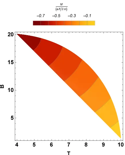
Figure 7.Magnetization along the first iso-magnetic trajectory as a function ofTin the range of 4Kto 10K. We select the different values forB2that we obtain from numerical calculations.
For the starting point previously indicated, we can consider a cycle for the degenerate case like that in Fig. 1operating between the temperatures 4K and 10 K. However, due to the behavior of temperature along the adiabatic trajectory described in Fig. 2, initially we brought the system into thermal equilibrium atT1 > T3. Thus, for that case, the heat defined byQ4→1corresponds to the heat absorbed, and for the heat released the correct definition is given byQ2→3, contrary to the non-degenerate case. To reinforce this idea, we display in the right frame of Fig.4the behavior of heat along the cycle for the degenerate case and non-degenerate case. The convention of the sign (positive for heat absorbed) is satisfied along the entire operation of the engine. The positive work condition, which plays an essential role for a wheel defined thermal engine, is shown in the left frame of Fig.4
for both cases. From the same figure, we can extract relevant information about therparameter. For a machine operating between two reservoirs of 4Kand 10K, we obtain
rmaxno−deg=1.58 and rmaxdeg =4.47, (34) which represents the maximum value that can be taken for the compression ratio along the cycle and corresponds to the point where the Carnot efficiency is obtained. These results are natural only to see the Fig.(3)for this example. For the non-degenerate case, it is only necessary to increase the field by a factor of 2.5, but for the degenerate case it is necessary to increase the field by a factor of 20 to reach the Carnot efficiency of the problem.
In Fig.5we compare the three efficiencies, where we see the effect of the degeneracy. One form to understand this behavior corresponds to the approximation that we show in Appendix A for the parametric solution, with the finality to “uncouple” the solution to magnetic field and the temperature for the adiabatic trajectory getting a function in the form
B(T) = k 2C1
1−e−k
q0.64
T2 (1−eTk)
, (35)
where we definek=eC2. So for this exponential form for the field as a function of temperature, when we parametrize the efficiency vs. a function of the typical compression ratio (r), we obtain the behavior present in Fig.5.
For the definition of works and its interpretation asW=−R
MdB, we study the magnetization along the cycle defined as
M= eh¯ 2m
2 β¯hωB
−coth
β¯hωB 2
. (36)
that the values of magnetization are always negative and the same occurs for the different curves in the “isomagnetic” process, shown in Fig.7, indicating that the response of the system is diamagnetic.
Our system was studied to prove a concept rather than a practical implementation protocol. However, we believe the readers will find attractive the study of the optimization of this cycle in degenerate conditions, following the work of Kosloff and Rezek [21] for the case of frictionless adiabats using the methods of shortcuts to adiabaticity [28].
5. Conclusions
In this work, we explored the possibility of constructing a single-particle quantum engine of the Landau problem. In particular, we found an analytical solution for the dependence of the magnetic field and temperature in the adiabatic trajectories. We use this relation to obtain the form of the efficiency showing a radically different behavior of the typical harmonic case and find that a major increase in the external magnetic field to reach the Carnot efficiency is necessary. We remark that the useful work of this engine, related to change in the magnetization along the process, can be used for example in the generation of induction current in other physics systems.
It is important to note that our one-particle approach must be refined to take into account a many electrons scenario, which yields more precise calculations. However, the one electron case is important due to simplicity and enrichment of physics for comparatives cases. For instance, we can work with a one-particle system combining the effects of a cylindrical potential well, which physically represents an accurate model for a semiconductor quantum dot, and an externally imposed magnetic field, where the number of electrons can be controlled without problems; thus, the same analysis presented in this work can be replicated.
Acknowledgments:F. J. P. acknowledges the financial support of FONDECYT-postdoctoral 3170010. A. S. N. and P.V. acknowledeges funding from FONDECYT 1150072 and support from Financiamiento Basal para Centros Científicos y Tecnológicos de Excelencia, under Project No. FB 0807 (Chile)
Author Contributions:F. J. P. and P. V. conceived the idea and formulated the theory. A. G. built the computer program and edited figures. R. G. R. solved the differential equation and their respective asymptotic analysis. A. S. N. and P. A. O. contributed to discussions during the entire work and the corresponding editing of the same. F. J. P. wrote the paper. All authors have read and approved the final manuscript.
Conflicts of Interest:The authors declare no conflict of interest.
Appendix A
We need to solve the differential equation in the form
dB dT =−
C21BT23csch 2
C1BT
1
B−C12TB2csch 2
C1BT
. (A1)
We define the parameteru=C1
B T
. So, differentiating respect toT, we obtain du
dT =−C1 B T2+
C1 T
dB
dT. (A2)
Collecting these two last equations, we obtain the first order differential equation in theuparameter in the form
du dT =
u
Tu2csch2(u)−1, (A3)
which corresponds to a differential equation of separable variables that has a solution given by
Figure A1.A parametric solution of the differential equation along the adiabatic trajectories for the Landau case. The dotted line represents the exact solution and the dot-dashed line the asymptotic case foru<<1. We can clearly see the constant value 0.5 for the solution in the case ofu>>1 from the dotted line in the figure. The solid line represents the proposal curve given by the Eq.(A13) showing a good fit for the problem under study.
whereC2is a constant of integration. We can compact this solution if we define the two variables
y= C1B
k x=
T
k, (A5)
wherekis given by
k=eC2, (A6)
with e as the Euler number. So, the solution takes the parametric form
y=e−ucothusinhu x= 1 ue
−ucothusinhu. (A7)
The asymptotic behaviors of these solutions is very interesting. The expression in the case ofu<<1, which corresponds to high-temperature or small magnetic field limit, takes the form
y= 1 e
q
6(1−ex), (A8)
so, we have a critical value,xc, wheny→0 given by
xc= 1
e. (A9)
It gives us a critical temperatureTcwhen the magnetic field goes to zero, and is strongly dependent on initial values of the problem under study, given by
Tc= k e ≡e
In the other case, foru>>1, which corresponds to low temperature or high magnetic field limit, we obtain
yc= 1
2, (A11)
and, this represents a critical constant value for the magnetic field, given by
Bc= k 2C1 ≡
eC2
2C1, (A12)
Thus, it is important to keep in mind that, when we consider a variation of the magnetic field as the cause for effective work in the system, the limits discussed before impose physical variable restrictions to operate the quantum machine proposed in the text.
To understand the magnetic field behavior in an explicit form along the adiabatic process, we propose an approximated curve in the form
y= 1 2
1−e
−√0.64(1−ex)
x
. (A13)
The exact parametric solution, the asymptotic behavior for the limiting cases(u>>1 andu<<1) and our proposal function are displayed in Fig.(A1).
References
1. Scovil, H. E. D.; Schulz-DuBois, D. O. Three-Level masers as a heat engines.Phys. Rev. Lett.1959,2, 262-263. 2. Huang, X. L.; Niu, X. Y.; Xiu, X. M. and Yi, X. X. Quantum Stirling heat engine and refrigerator with single
and coupled spin systems.Eur. Phys. J. D2014,68, 32.
3. Su, S. H.; Luo, X. Q.; Chen, J. C. and Sun, C. P. Angle-dependent quantum Otto heat engine based on coherent dipole-dipole coupling.EPL2016,115, 3, 30002.
4. Roßnagel, J.; Bah, O.; Schmidt- Kaler, F.; Singer, K.; Lutz, E. Nanoscale heat engine beyond the Carnot limit.
Phys. Rev. Lett.2014,112, 030602.
5. Scully, M. O.; Zubairy, M. S.; Agarwal, G. S.; Walther, H. Extracting work from a single heath bath via vanishing quantum coherence.Science2003,299, 862-864.
6. Scully, M. O.; Zubairy, M. S.; Dorfmann, K. E.; Kim, M. B.; Svidzinsky, A. Quantum heat engine power can be increased by noise-induced coherence.Proc. Natl. Acad. Sci. USA2011,108, 15097-15100.
7. Bender, C. M.; Brody, D. C. and Meister, B. K. Quantum mechanical Carnot engine.J. Phys. A: Math. Gen.
2000,33, 4427.
8. Bender, C. M.; Brody, D. C. and Meister, B. K. Entropy and temperature of quantum Carnot engine.Proc. R. Soc. Lond. A 2002,458, 1519.
9. Wang, J. H.; Wu, Z. Q. and He, J. Quantum Otto engine of a two-level atom with single-mode fields.Phys. Rev. E 2012,85, 041148.
10. Huang, X. L.; Xu, H.; Niu, X. Y. and Fu, Y. D. A special entangled quantum heat engine based on the two-qubit Heisenberg XX model.Phys. Scr. 2013,88, 065008.
11. Muñoz, E. and Peña, F. J. Quantum heat engine in the relativistic limit: The case of Dirac particle.Phys. Rev. E 2012,86, 061108.
12. Muñoz, E.. and Peña, F. J. Magnetically driven quantum heat engine.Phys. Rev. E 2014,89, 052107. 13. Peña, F. J. and Muñoz, E. Magnetostrain-driven quantum heat engine on a graphene flake.Phys. Rev. E 2015,
91, 052152.
14. Peña, F. J.; Ferré, M.; Orellana, P. A.; Rojas, R. G. and Vargas P., Optimization of a relativistic quantum mechanical engine.Phys. Rev. E 2016,94, 022109.
15. Wang, J.; He, J. and He. X. Performance analysis of a two-state quantum heat engine working with a single-mode radiation field in a cavity.Phys. Rev. E 2011,84, 041127.
16. Abe, S., Maximum-power quantum-mechanical Carnot engine.Phys. Rev. E 2011,83, 041117.
18. Wang, R.; Wang, J.; He, J. and Ma, Y. Performance of a multilevel quantum heat engine of an ideal N-particle Fermi system.Phys. Rev. E 2012,86, 021133.
19. Callen, H. B.Thermodynamics and an Introduction to Thermostatistic; Jhon Wiley and sons: New York, USA, 1985.
20. Tolman, R. C.The Principles of Statistical Mechanics; Oxford University Press: Oxford, UK, 1938. 21. Kosloff, R. and Rezek, Y., The Quantum Harmonic Otto Cycle.Entropy2017,19, 136.
22. Roßnagel, J.; Dawkins, T. K.; Tolazzi, N. K.; Abah, O.; Lutz, E.; Kaler-Schmidt, F.; Singer. K. A single-atom heat engine.Science.2016,352, 325.
23. Kumar, J.; Sreeram P. A. and Dattagupta, S., Low-temperature thermodynamics in the context of dissipative diamagnetism.Phys. Rev. E 2009,79, 021130.
24. Mehta, V. and Johal, R. S. Quantum Otto engine with exchange coupling in the presence of level degeneracy.
Phys. Rev. E 2017,96, 032110.
25. Muñoz, E.; Peña, F.J.; González, A. Magnetically-Driven Quantum Heat Engines: The Quasi-Static Limit of Their Efficiency. Entropy2016,18, 173.
26. Quan, H. T. Quantum thermodynamic cycles and quantum heat engines. II.Phys. Rev. E 2009,79, 041129. 27. Zheng, Y. and Polleti, D. Work and efficiency of quantum Otto cycles in power-law trapping potentials.Phys.
Rev. E 2014,90, 012145.