Supervised Ranking of Co-occurrence Profiles for Acquisition of
Continuous Lexical Attributes
Julian Brooke
Department of Computer Science University of Toronto [email protected]
Graeme Hirst
Department of Computer Science University of Toronto [email protected]
Abstract
Certain common lexical attributes such as polarity and formality are continuous, creating chal-lenges for accurate lexicon creation. Here we present a general method for automatically placing words on these spectra, usingco-occurrence profiles, counts of co-occurring words within a large corpus, as a feature vector to a supervised ranking algorithm. With regards to both polarity and formality, we show this method consistently outperforms commonly-used alternatives, both with respect to the intrinsic quality of the lexicon and also when these newly-built lexicons are used in downstream tasks.
1 Introduction
Lexicon acquisition represents one key way that the information in large corpora and other resources can be leveraged in various NLP tasks, particularly when the range of lexical items involved in a particular phenomenon is much more diverse than can typically be captured in manually-built resources. Another property of the lexicon which might limit a manual approach is the fact that certain attributes are not discrete, instead falling on a continuous spectrum; although there are manually-built dictionaries which contain fine-grained judgments of spectra—an example is the MRC psychological database (Coltheart, 1980)—these tend to be very low in coverage, reflecting the difficulty in collecting this information.
Within computational linguistics, the continuous lexical attribute that has received the most attention is undoubtedly the positive-negative spectrum, otherwise known assemantic orientation(SO) orpolarity. Much of the work focused on acquisition of this attribute at the lexical level has involved simplification to a binary (positive-negative) or ternary (positive-neutral-negative) distinction (Hatzivassiloglou and McKeown, 1997; Takamura et al., 2005; Kaji and Kitsuregawa, 2007; Rao and Ravichandra, 2009; Mohammad et al., 2009; Volkova et al., 2013) but other work explicitly offers a continuous quantification (Turney, 2002; Turney and Littman, 2003; Baccianella et al., 2010). Another spectrum with a prominent role in the lexicon isformality(Brooke et al., 2010; Lahiri et al., 2011), which includes colloquial words at one end, socially-distancing words at the other, and common vocabulary in the middle. In this paper, we will focus on these two spectra; the method presented, however, is intended to be general, and as such could be easily applied to other spectra such as those in the MRC database, e.g. abstractness (Turney et al., 2011), and other kinds of variation captured in, for instance, Osgood’s semantic differential (Osgood et al., 1957).
The typical approach to this problem involves semi-supervised methods using vector space and/or graph representations and a set of seed terms. Our method is novel in that it uses fully supervised SVM ranking of co-occurrence profiles, i.e. normalized counts of instances of binary text co-occurrence between the target word and a large set of profiling words, selected on the basis of their frequency, in a publicly-available blog corpus. The seed terms from earlier methods are now viewed as training examples for building a supervised model that can connect the distributions of co-occurring words in this wider vocabulary to relative locations on a continuous spectrum. This approach depends somewhat upon improved manual lexical resources available for these tasks, such as the SO-CAL dictionary (Taboada This work is licenced under a Creative Commons Attribution 4.0 International License. Page numbers and proceedings footer are added by the organizers. License details:http://creativecommons.org/licenses/by/4.0/
et al., 2011) in the case of polarity, but we limit our (word) training set size in order to show it will work in resource-scarce situations, such as languages other than English. Our method is straightforward, practical, and offers essentially full coverage, including words and lexicogrammtical patterns that are simply not accessible by the many popular methods that are primarily based on WordNet.
To evaluate, we compare our method with popular alternatives in both polarity and formality, with particular emphasis on other methods based on corpus co-occurrence that have also been shown to be generalizable across various spectra, i.e. LSA and PMI. For both spectra of interest here, we evaluate both intrinsically using pairwise comparisons from manually-built lexical resources, and also extrinsically in downstream tasks such as text-level polarity classification and sentence-level formality judgments. We show our method is consistently superior across our various evaluations. We also show that not only are co-occurrence profiles a good source of information for supervised ranking, but that a focus on ranking rather than regression in this space appears to be fundamental to the success of a supervised approach to lexical spectra.
2 Related Work
Viewed primarily as a categorical task, the creation or expansion of lexical resources for sentiment anal-ysis is a commonly-addressed problem. In addition to SentiWordNet (Baccianella et al., 2010), which we will compare to directly to here, there are numerous mostly semi-supervised approaches based on exploiting the glosses and/or the graph structure of WordNet to determine whether a word is positive or negative (Kamps et al., 2004; Hu and Liu, 2004; Kim and Hovy, 2004; Takamura et al., 2005; An-dreevskaia and Bergler, 2006; Rao and Ravichandra, 2009; Hassan and Radev, 2010), or taking advan-tage of some other lexicographic resources (Mohammad et al., 2009; Klebanov et al., 2013). The earliest corpus-based approach was that of Hatzivassiloglou and McKeown (1997) who used local syntactic in-formation, i.e. conjunctions, to make connections between adjectives; other work that makes use of local patterns in a corpus includes that of Kaji and Kitsuregawa (2007) and Kanayama and Nasukawa (2006). Turney (2002) built a continuous polarity lexicon using PMI based on Internet hit counts as a useful measure of relatedness between seeds, and Turney and Littman (2003) compared this approach with LSA, which uses general patterns of co-occurrence based on dimensionality reduction. Velikovich et al. (2010) combined web-scale corpora with a graph-based approach, assigning polarity scores ton-grams on the basis of the maximum weighed path from ann-gram to the seed terms, using a small (6-word) context around the word. Like us, Volkova et al. (2013) use social media, iteratively labeling tweets and words for subjectivity and polarity. Fully-supervised approaches to polarity lexicon acquisition are rare, but one example is the work of Chetviorkin and Loukachevitch (2012), who classify words as being sentiment-relevant in Russian using a small set of statistical features, including ratios across disparate corpora.
Our interest in the continuous aspect of polarity overlaps with work on deriving the semantic intensity of lexical items from corpora (Sheinman and Tokunaga, 2009); in this task, small sets of synonyms are ranked according to their intensity, including (but not limited to) polarity. De Melo and Bansal (2013) use a Mixed Integer Linear Programing algorithm to combine information from multiple pairs into a single coherent ranking. As with some of the work in polarity, the focus is on adjectives and local patterns which explicitly distinguish degrees of intensity e.g.not only x but also y, which limits its range of application; it would not, for instance, be useful for formality or other more pragmatic variations.
also relevant to the recent interest in identifying social relationships (Peterson et al., 2011) and shows of politeness (Danescu-Niculescu-Mizil et al., 2013).
3 Method
Our approach to lexicon acquisition falls into the general category of corpus-based techniques. For both attributes addressed in this paper, we use the same corpus, the 2009 ICWSM Spinn3r dataset (Burton et al., 2009), a publicly-available blog corpus which we also used in our earlier work on lexical formality (Brooke et al., 2010). Blogs are a good resource for broad lexical acquisition because they are very broad in style and content, and are available in essentially unlimited amounts. We use the English Tier 1 (high-quality) blogs that have at least 100 word types, excluding duplicate texts; after this filtering, our dataset contains a total of about 2.4 million blogs.
To build a lexicon for any continuous attribute of interest, we begin by creatingco-occurrence profiles
as follows: First, we select a document frequency rangemin-df,max-df that determines a set of profile words Pin a corpus S, where for each p∈P, the document frequency dfS
p of pin S is limited to be
min-df <dfSp<max-df; that is, each profile word appears in more thanmin-df documents, but fewer thanmax-df documents in our corpus. Then, given a sample sizenand a target wordwthat we wish to profile, we sample a set ofntexts fromSwhich contain the target word (or all the documents where the word appears, if it appears fewer thanntimes), and count the document frequency of each profile word
pin this subcorpus, Tw. We ignore the term frequencies within individual documents because a binary representation is known to be preferred for stylistic dimensions like formality (Brooke et al., 2010), and this seems to be also somewhat true in the domain of polarity, where better results can be obtained when multiple instances of a polar word are discounted (Taboada et al., 2011). To avoid overfitting our statistical model, we do not count a word as appearing with itself. Once we have sub-corpus document frequencesdfTw
p for each p, for each profile word pwe define the element of our co-occurrence profile vectorvpas
vp= df Tw
p
∑q∈PdfTqw
That is, we normalize each count by the sum across all counts, such that the L1 norm ofvis 1. For our applications here, the dimension of the co-occurrence profile vector is typically in the tens of thousands, but to illustrate the creation of this vector, suppose we choose an extremely narrow document frequency bandmin-df,max-df, such there were only three co-occurrence profile words: p1,p2,p3. For some word
w, we sample n instances of texts from our corpus which contain w, and find that p1 appears in 10
of these texts, p2 in 40 of them, and p3 in 50 of them. The resulting co-occurrence profile vector is v=h0.1,0.4,0.5i. This profile could be viewed as a distributional vector space representation of the word (Turney and Pantel, 2010), or as an estimate of the probability of eachpoccurring withw; without any further manipulation, however, we will use it directly as a feature vector for our supervised ranking. In order to proceed with a supervised approach, we need a ranking of a set of words relevant to the lexical attribute that we wish to acquire; this ranking is specific to the attribute in question, so we discuss this in later sections. Given such a ranking (which, we note, may be partial), we applySVMrank
(Joachims, 2002), which is part of the SVMlight set of SVM-based machine learning tools. SVMrank was developed for ranking web page results, and, to our knowledge, has not been applied in this space.
SVMrankuses an algorithm which optimizes the Kendall’sτ(Kendall, 1955) between a correct rankingra and the automatically-generated rankingrb. The simplest version ofτis based on the number of pairwise rankings which are in concord (C), i.e. both rankings rank the pair relative to each other and the pairwise rankings are the same, or in discord (D), i.e. both rankings rank the pair relative to each other but the rankings offered are contradictory.τis defined as:
In practice, this is accomplished inSVMrankby modifying the original SVM algorithm to use as feature vectors the difference between ranked input vectors, rather than the input vectors directly. In the context of this feature space, this means that the model is trained on vectors which represent the differences in the co-occurrence profiles of ranked words; if the word with co-occurrence profileuis ranked higher than a word with co-occurrence profilevin our annotation, thenSVMrankwill try to find a weight vector w such that(u−v)·w>0, wherewis constrained to be a sum of co-occurrence profile differences (i.e. the support vectors). Like standard SVM, ranking SVM uses aCparameter which represents the trade-off between margin size and classification errors, though the interpretation of the margin in ranking SVM is less clear. The output of the classification step ofSVMrank is a number for each word which can be used directly to rank words, or which can be normalized across words into a scale. If the input rankings also have a continuous numerical representation (which is true in our case for polarity), then this ranking approach can be compared directly to a standard regression which is not directly sensitive to rankings; to maximize comparability, we use the regression function included inSVMlight for this purpose. For both, we used a linear kernel.
There is a small number of parameters that need to be set: the sample size n, the frequency range
min-df,max-df, and the SVMCparameter. For each of the two lexical attributes of interest, we carried out independent tuning of these parameters using 5-fold crossvalidation in the training set, carrying out a grid search at powers of 10. We will discuss the values of parameters with respect to specific experiments later, but we mention here that a higher-than-defaultC, which corresponds to more emphasis on avoiding error rather than maximizing the margin, gave better results for both ranking and correlation, though with diminishing returns. The role ofnis primarily to make the method (much) more tractable, but we suspect it might be beneficial to the training of the model for the profiles to be based on a uniform number of examples across word types.
Before we move on to the experimental evaluation, we highlight some intrinsic advantages of this model, independent of performance. As a technique based on large corpus co-occurrence, it has the im-portant property that it can go beyond the limited vocabulary offered by, for instance, WordNet. Since we rely only on co-occurrence, we are not at all limited to individual words (or specific types of words): we could just as easily derive attribute values forn-grams, collocations, or full lexico-grammatical con-structions (for instance, distinguishinghighas related topricefromhighas related toquality); though our interest here is in general lexical properties, there is no reason this approach could not be used for domain-specific applications, for any lexical units that appear often enough to obtain a reliable co-occurrence profile. Unlike many graph-based techniques, new vocabulary can be classified directly with-out perturbing the model, potentially in an online fashion if the corpus is properly indexed (which, we note, is by far the most time-consuming step of our method). Though some lemmatization may be re-quired for highly inflectional languages, the method extends easily to any language for which blog data is likely to be available in sufficient quantities. Our approach is more straightforward than most other methods based on co-occurrence, which means fewer arbitrary choices and nuisance variables (such as the dimensionalitykor feature weighting typically used in dimensionality-reduction approaches such as LSA); the parameters that we have are fairly well-behaved. Unlike methods which rely only on examples from the extremes of a spectrum to derive a quantification of it, our method naturally integrates examples from the middle of the spectrum (e.g. neutral examples in the case of polarity), but does not inherently require fine-grained quantification of the entire spectrum; in fact, pairwise examples alone could be used for training.
4 Polarity experiments 4.1 Word-level Evaluation
adjec-tives), and we randomly select only 50 words from each of the 11 possible SO ratings in the dictionary (for a total of 550 words), so as to mimic a (relatively) low-resource situation as we might find working in other languages, and to make it possible to keep the counts equal across SO ratings. Note that the SO-CAL dictionary does not contain neutral words (words not in the dictionary are assumed to be neutral), but we used a set of about 200 hand-marked neutral adjectives that had been excluded from the lexicon during its creation from the words in a set of Epinions product reviews, and which were used for the original dictionary evaluation by Taboada et al. (2011).
After training our model, we evaluate in two test sets. The first test set is the rest of the SO-CAL dictionary, excluding words in the training set as well as those not given a rating by SentiWordNet (see below). Note that this set is not balanced across SO values, since there are many more weakly positive (SO 1 to 3) or weakly negative (SO −1 to −3) words than more-extreme or neutral words; we would argue, though, that this reflects the actual situation in subjective corpora such as product reviews. To test whether we might be overfitting to the product reviews domain, we also test using annotations from the MPQA (Subjectivity) lexicon (Wilson et al., 2005), which was built primarily from news texts.1For this,
we again include only words that are in SentiWordNet. The MPQA lexicon uses a very different tagging schema than the SO-CAL dictionary, with 3 polarity categories (positive, negative, and neutral) as well as two degrees of subjectivity, weak or strong. Strong or weak subjectivity is defined as how reliable an indicator of subjectivity the word is, which does not directly correspond to the rationale used for the SO-CAL dictionary (which is closer to the notion of force or intensity); the results in Taboada et al. (2011) and our own examination of the lexicon suggest, however, that there is some correlation.2Despite
this uncertainty, we combined the MPQA tags to form a polarity spectrum: strongly subjective negative, weakly subjective negative, neutral, weakly subjective positive, strongly subjective positive. Given a ranking by our SVM ranker, we evaluate overall pairwise accuracy by considering all possible pairings of words across different ratings within the SO-CAL or MPQA test sets, and count the percentage of those where the ordering of the pair with respect to the polarity spectrum is correctly predicted by the ranking. For a more detailed breakdown, we divide these pairwise comparisons into 3 categories: polarity (pairs which involve one positive and one negative word), neutrality (pairs which have one neutral word), and intensity (pairs which have two words with the same polarity). Note that much work in bootstrapping lexicons for sentiment analysis uses precision and recall, but this is not the most appropriate evaluation metric in this case because our method can assign a rank (and, eventually, an SO value) to any word in the 2 million word vocabulary of our corpus.3Here, we are interested only in reliability of these rankings.
During parameter tuning in the development phase, we found thatmin-df =103,max-df =105was a
good choice: in other words, our profile words are words that appear less than once in 24 texts, but more than once in 2400 texts. In the ICWSM, there are 30,852 words that fall into this category, so that is the length of our feature vector. Based on results in the development set, we taken=1000 as our default; larger samples provided no appreciable benefit and were even slightly worse in some cases. For the SVM
Cparameter, we used 100. We also test using SVM correlation, using the same parameters.
In addition to these variations on our co-occurrence profile technique, we also compare with three independent alternatives. The first is SentiWordNet 3.0 (Baccianella et al., 2010), which uses a random walk method in WordNet to derive positive, negative, and neutral values (which sum to 1) for each synset in WordNet. We follow Taboada et al. (2011) in converting this to a single spectrum for each word by subtracting the negative score from the positive score, and averaging the result across senses for each
1There are of course other popular manually-built lexicons, for instance the General Inquirer (Stone et al., 1966), but they
tend to have only binary annotations.
2One example of where these two dictionaries differ is the wordnervous, which is tagged as a strongly subjective negative
word in the MPQA, but has only a−1 score in the SO-CAL dictionary, since it does not describe a particularly intense negative emotion. An example of a−5 word ishorrendous, which is also a strongly subjective negative word in the MPQA. Instances of discord where the SO-CAL dictionary is clearly stronger are rarer, but an example iscomprehensive, which has an SO of 3 in SO-CAL, but is weakly subjective in the MPQA, probably because of its common descriptive uses, such as in the context of insurance and (in the UK) education.
3We have not yet build such a lexicon, but, to facilitate comparison, but we are making available raw scores for all the
adjectives already contained in at least one of the SO-CAL, MPQA, and SentiWordNet lists (excluding the 550 training words), as well as lists of specific words used for training and testing. These resources can be found at http://www.cs.toronto.edu/
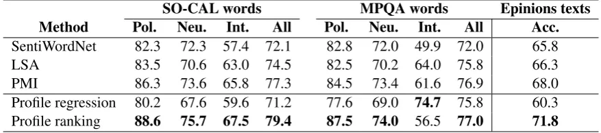
Table 1: Results of polarity experiments. Left side of table shows pairwise accuracy (%) for various sentiment lexicon ranking methods in SO-CAL and MPQA test sets. Pol. = Pairs with different polarity; Neu. = Pairs with at least one neutral word; Int. = Pairs with the same polarity, but different intensi-ties. Right side of table shows text polarity classification accuracy (%) in Epinions Corpus for various adjective lexicons. Bold is best in column.
SO-CAL words MPQA words Epinions texts
Method Pol. Neu. Int. All Pol. Neu. Int. All Acc.
SentiWordNet 82.3 72.3 57.4 72.1 82.8 72.0 49.9 72.0 65.8
LSA 83.5 70.6 63.0 74.5 82.5 70.2 64.0 75.8 66.3
PMI 86.3 73.6 65.8 77.3 84.5 73.4 61.6 76.9 68.0
Profile regression 80.2 67.6 59.6 71.2 77.6 69.0 74.7 75.8 60.3
Profile ranking 88.6 75.7 67.5 79.4 87.5 74.0 56.5 77.0 71.8
word (in that paper, they also considered using only the most common sense but found the results to be indistinguishable). The second alternative uses the semi-supervised LSA-based method of Turney and Littman (2003). For the first step, singular value decomposition, we use a binary term-document matrix with the same ICWSM texts as our supervised model, withk=500 (a fairly standard choice). In the second step, which involves calculating the cosine similarity with a set of seed terms using the LSA vectors and then taking the difference, the positive and negative seeds are just the training instances for our supervised model (neutral terms are discarded). Our third comparison is the PMI approach of Turney (2002), which is still popular: for instance, PMI was used to built a Twitter sentiment lexicon in the winning entry in a recent shared task (Mohammad et al., 2013). Because they have access to the same corpus and even the same example words as our method, the LSA and PMI alternatives are most directly comparable to ours.
The results for the word-level polarity experiments are shown in the left side of Table 1. In the SO-CAL test set, the results are clear: our SVM ranking method is preferred over alternatives, across all the different categories of pairwise comparison. The relative difficulty of each pair type reflects the average distance between relevant pairs on the spectrum, as expected. Surprisingly, the correlation method, despite using the same feature input as the ranking method, is the worst performing method here, though SentiWordNet is only marginally better, while LSA falls roughly in the middle of the range, and PMI is the strongest competitor. One potential criticism is that a ranking method is likely to have an advantage when evaluating by rank. This is true, but we think that relative rank among words is fundamental to the notion of a spectrum, whereas the bucketing of words into evenly spaced integer ratings is just an annotation convenience. That said, our output ranking is perhaps too fine-grained in comparison to our input (offering a full ranking for all words), and it would be desirable if our ranking algorithm allowed us to encourage some words to be ranked the same.
4.2 Text-level Evaluation
The most common use of polarity lexicons is the task of text polarity classification (Turney, 2002), identifying whether an opinionated text is positive or negative. In this section, we convert the initial output of the models to polarity lexicons with an appropriate scale so that we can use the SO-CAL software (Taboada et al., 2011) to carry out text sentiment analysis with our alternative adjective lexicons rather than its original, manually-built one. SO-CAL is an unsupervised lexical sentiment analysis system with a number of built-in features, e.g. handling of negation and intensification, that improve the accuracy of the model, particularly when using a fine-grained, high-precision lexicon. Taboada et al. evaluate across 4 corpora of balanced product reviews. For our evaluation, we use one of those corpora, a set of 400 product reviews from Epinions, with 50 balanced texts from each of 8 product categories (movies, books, cars, computers, cookware, hotels, phones, and music). Taboada et al. call this corpus Epinions 2, to distinguish it from the Epinions corpus that the SO-CAL dictionary was built from. They report an accuracy of 80% using SO-CAL with all word types and features enabled.
Our interest here is to test the influence of lexicon quality on polarity detection. Coverage, though of course important, is actually a potential source of noise: Low coverage can naturally result in low performance, but Taboada et al. point out that high coverage can also cause problems, when many of the rarer words added to the lexicon, even when human-tagged, are not relevant to the primary sentiment of the text, but rather irrelevant aspects like (in the movie or book domain) character descriptions. Steps can be taken to mitigate this by identifying relevant sentiment (Scheible and Sch¨utze, 2013), but here we sidestep this problem by forcing our lexicons to have exactly the same coverage by limiting them to words that appear in the static SentiWordNet lexicon. Again, we also consider only adjectives here.
To build the lexicon for this evaluation we used a different training set: it is not possible to take 50 samples from each SO rating in the SO-CAL adjective lexicon and not have training words that also appear in the corpus, which we explicitly wanted to avoid.4 Instead, we train using all the adjectives in
the SO-CAL dictionary that either don’t appear in the Epinions corpus or don’t appear in SentiWordNet (since we are limiting our output lexicon to SentiWordNet words). This results in a much larger training set than in the word-level evaluation (about 1500 words), but they are distributed unevenly across SO ratings. Relative to the word-level evaluation, this is closer to the situation if we were using the entire SO-CAL dictionary to expand the lexicon. We use the same set of training words as seeds for LSA.
To convert SentiWordNet to a SO-CAL-compatible dictionary, we simply multiply the raw score, guaranteed to be between−1 and+1, by 5, creating a range of−5 to+5. For the raw scores for our other three options (LSA, profile regression, and profile ranking), we linearly scale the raw score so that the mean within the lexicon is 0, and a SO+5 word is at the third standard deviation away from the mean; we choose a rather severe scaling so that there are only a handful of words in the lexicon whose absolute value is over 5, which SO-CAL is not designed for.
The results of this evaluation are shown on right side of Table 1. Profile ranking is once again dom-inant, almost 4 percentage points better than the second-best option. The ordering of the lexicons here is exactly the same as we saw for the word-level evaluation in SO-CAL, though SentiWordNet does somewhat better than would be expected from those scores. Again, regression does quite poorly despite having access to the same feature vectors as the ranking method. We note that our results here are also markedly better than all the other automatic lexicons compared by Taboada et al., namely a PMI-derived lexicon based on Google counts (Taboada et al., 2006), and a binary lexicon built by expanding entries in a thesaurus (Mohammad et al., 2009), and are even a bit better than using the human-tagged (binary) annotations from the General Inquirer (Stone et al., 1966), though we are still quite a long way from what is possible with the full manual SO-CAL dictionary. Since the quality of the lexicon is directly reflected in our polarity classification scores here, it is not surprising that our gold-standard lexicon is superior; in this context, it should be viewed as an upper bound. Nevertheless, we have strong evidence here that our co-occurrence profile ranking method is a step in the right direction relative to other methods for automatically building lexicons.
4For all of our evaluations in this paper we were careful never to use the score of a word which appeared in our training set;
5 Formality Experiments 5.1 Word-level Evaluation
Though the lexicon is perhaps more fundamental to distinctions of polarity than is the case for formality, nevertheless formality is strongly expressed through word choice; for instance, in English using the word dude to address a socially-powerful stranger would generally be unacceptable, and it would be very strange to address a good friend assir, except as a joke. These are not isolated examples: a huge portion of the vocabulary is marked to some degree in this fashion, and requires special attention when moving across text genres or social situations. Word length (in English, at least) and word frequency can be used as a simple proxy (longer, rarer words are, on average, more formal), but the example above belies this approach: sir is a shorter word than dude, and it is not immediately obvious that it would appear less in, for instance, a news corpus, thandude.
In previous work (Brooke et al., 2010), we used the LSA co-occurrence method of Turney and Littman (2003) discussed in the previous section to derive a formality lexicon using the ICWSM (which was the best among various corpora tested, including the BNC). For testing, we used a set of 399 synonym pairs that were pulled from a writing manual focused on word choice,Choose the Right Word(CTRW) (Hayakawa, 1994), where the author explicitly compared words for their formality, showing that co-occurrence was a better approach to identifying lexical formality than proxies related to word length or word frequency. We note that many of the distinctions in the CTRW set are quite subtle, for example
determinevs.ascertain, both of which seem at least somewhat formal, thoughascertainwas judged by the expert to be the more formal of the two. In this section we will build a formality ranking using our profile ranking method, and show that it is better than the LSA method in the CTRW dataset. Here, we follow our earlier work in using a much smaller k value (20) than is typical for topical uses of LSA, which we found was better for this dataset, since major stylistic differences seem to be mostly captured in the first few dimensions after dimensionality reduction, a result which is consistent with the work of Biber (1988) looking at differences across registers.
Unlike for polarity, there is no resource available that offers a full scale of formality for a large number of words, and the set used in our initial work on formality has only extreme, handpicked words. In more recent work (Brooke and Hirst, 2013), we used a larger set of words (900) that included a variety of different styles that had been tagged by a group of 5 annotators. In that work, we did not use the term “formality,” but one of our styles, colloquial, corresponds to the informal end of the spectrum, and two other styles, objective andliterary, can both be viewed as social-distancing language.5 The
words tagged by annotators as belonging to neither of these categories will serve as the middle of this spectrum. Compared to our polarity lexicon, our training set therefore is much more coarse-grained (with only 3 rankings, as compared to 11 for polarity), but the pairwise relationships can be used to build a fine-grained scale. As before, we remove all words that overlap with our test set.
With respect to parameters, we use the samenas in the polarity experiments, but in development we saw better performance from a higherC(10,000) and a lower bottom bound on the document frequency range, df-min=102. The latter might reflect the fact that rare vocabulary has a strong tendency to be
associated with extreme formality, though there is also a limit to this, since if a word is so rare that it hardly ever co-occurs with anything, it cannot possibly be useful for training no matter how good an example of extreme formality it is. The results using these settings are shown in the left side of Table 2. Again, our profiling method is clearly better than lexicon-based alternatives. LSA outperforms PMI in the word-level task, a result which is consistent with our other work in stylistic lexical induction (Brooke and Hirst, 2013),6and all the co-occurrence methods are well above the word-length baseline.
Figure 1 contains a more detailed analysis of the influence of individual document frequency bands: we
5The objective dimension corresponds roughly to the style of a technical document, while the literary dimension involves
flowery, even archaic language that suggests a literary sophistication. Contrastsowith synonymstherefore(objective) andthus (literary), which are both more formal, but in different ways.
6We suspect this is due to the fact that LSA vectors encode information about word frequency: even when the vector norm is
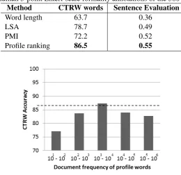
Table 2: Results of the formality experiments. The second column shows pairwise accuracy of different models identifying the more formal of two synonyms in CTRW test set. The third column shows average correlation with two human 5-point Likert-scale formality annotations of the 500 sentence test set.
Method CTRW words Sentence Evaluation
Word length 63.7 0.36
LSA 78.7 0.49
PMI 72.2 0.52
Profile ranking 86.5 0.55
Figure 1: Pairwise accuracy in the CTRW test set for various frequency bands. Dotted line represents performance using best parameters from development phase, i.e.max-df =102,max-df =105.
built models for each of our frequency bands (ranges between two consecutive powers of ten), and tested them in the CTRW corpus. The flat dotted line represents the larger band we used based on development performance, 102–105. We see that accuracy peaks at 103 to 104 df band, at a value (87.3%) which is
higher than we saw with the larger band chosen based on the development set. The words in this band are fairly uncommon, appearing less than once in 240 texts, but greater than once in 2400 texts; still, as a group they provide enough evidence to make a strong determination of formalty.
5.2 Sentence-level Evaluation
Lahiri and Lu (2011) report on the creation of 5-point Likert scale annotations of sentence-level formality, with two ratings for each of 500 sentences taken from separate texts in a diverse corpus which includes news, blogs, forums, and academic papers (Lahiri et al., 2011). In this section, we use this annotation to carry out an extrinsic evaluation of our lexical formality ratings. As far as we are aware, this is the first use of this annotation for evaluating metrics of formality. We extract all lexical words (verbs, adjectives, adverbs, and nouns, though we omit proper nouns) from the sentences and use the 3-way formality annotation with these words removed to create LSA, PMI, and profile ranking models, which are then used to create a formality lexicon for these words, using the same method we used to create the SO lexicon. Given a lexicon, we averaged the formality score across each sentence (ignoring duplicate items) to get a formality score for each sentence. We calculate Pearson’s correlation coefficient between our score and each of the two annotators, and then average the result. For comparison, the correlation between the two human annotators is 0.60.
6 Conclusion
In this paper we have presented a novel approach to determining where a word lies on a spectrum, using just counts of words that it tends to appear with and an SVM ranking algorithm, both of which are key components to its success. We have shown that it can be applied to at least two continuous attributes of interest in computational linguistics, namely polarity and formality, and that the benefits of this method relative to established alternatives are visible not just in direct lexicon evaluation, but also in the NLP tasks where these lexicons can be used. Even with a relatively small set of words to train with, we see little sign of overfitting, and although we have focused on a small set of words here, our method is efficient enough that it could easily be applied to a much larger set of lexicogrammatical units, though we will also have to derive ways to filter out unreliable assignments to reduce overall noise. Other future work will involve looking at other spectra, other languages, other supervised ranking models, and improving our performance generally by being more selective of profile words or training examples or by refining our rankings by including other sources of information such as WordNet.
Acknowledgements
This work was supported by the Natural Sciences and Engineering Research Council of Canada and the MITACS Elevate program. Thanks to Shibamouli Lahiri and Maite Taboada for the use of their resources and their feedback.
References
Alina Andreevskaia and Sabine Bergler. 2006. Semantic tag extraction from WordNet glosses. InProceedings of 5th International Conference on Language Resources and Evaluation (LREC ’06).
Stefano Baccianella, Andrea Esuli, and Fabrizio Sebastiani. 2010. SentiWordNet 3.0: An enhanced lexical re-source for sentiment analysis and opinion mining. InProceedings of the 7th Conference on International Lan-guage Resources and Evaluation (LREC’10), Valletta, Malta, May.
Douglas Biber. 1988.Variation Across Speech and Writing. Cambridge University Press.
Julian Brooke and Graeme Hirst. 2013. Hybrid models for lexical acquisition of correlated styles. InProceedings of the 6th International Joint Conference on Natural Language Processing (IJCNLP ’13).
Julian Brooke, Tong Wang, and Graeme Hirst. 2010. Automatic acquisition of lexical formality. InProceedings of the 23rd International Conference on Computational Linguistics (COLING ’10), Beijing.
Kevin Burton, Akshay Java, and Ian Soboroff. 2009. The ICWSM 2009 Spinn3r Dataset. InProceedings of the Third Annual Conference on Weblogs and Social Media (ICWSM ’09), San Jose, CA.
John Carroll, Guido Minnen, Darren Pearce, Yvonne Canning, Siobhan Devlin, and John Tait. 1999. Simplifying English text for language impaired readers. InProceedings of the 9th Conference of the European Chapter of the Association for Computational Linguistics (EACL’99).
Ilia Chetviorkin and Natalia Loukachevitch. 2012. Extraction of Russian sentiment lexicon for product meta-domain. InProceedings of the 24th International Conference on Computational Linguistics (COLING ’12). Max Coltheart. 1980. MRC Psycholinguistic Database User Manual: Version 1.Birkbeck College.
Cristian Danescu-Niculescu-Mizil, Moritz Sudhof, Dan Jurafsky, Jure Leskovec, and Christopher Potts. 2013. A computational approach to politeness with application to social factors. InProceedings of the 51st Annual Meeting of the Association for Computational Linguistics (ACL ’13).
Gerard de Melo and Mohit Bansal. 2013. Good, great, excellent: Global inference of semantic intensities. Trans-actions of the Association for Computational Linguistics, 1.
Ahmed Hassan and Dragomir Radev. 2010. Identifying text polarity using random walks. InProceedings of the 48th Annual Meeting of the Association for Computational Linguistics, (ACL ’10).
Vasileios Hatzivassiloglou and Kathleen R. McKeown. 1997. Predicting the semantic orientation of adjectives. In
S.I. Hayakawa, editor. 1994. Choose the Right Word. HarperCollins Publishers, second edition. Revised by Eugene Ehrlich.
Francis Heylighen and Jean-Marc Dewaele. 2002. Variation in the contextuality of language: An empirical measure.Foundations of Science, 7(3):293–340.
Minqing Hu and Bing Liu. 2004. Mining and summarizing customer reviews. InProceedings of the Tenth ACM SIGKDD International Conference on Knowledge Discovery and Data Mining (KDD ’04).
Thorsten Joachims. 2002. Optimizing search engines using clickthrough data. In9th ACM SIGKDD Conference on Knowledge Discovery and Data Mining (KDD ’02).
Nobuhiro Kaji and Masaru Kitsuregawa. 2007. Building lexicon for sentiment analysis from massive collection of HTML documents. InProceedings of the 2007 Joint Conference on Empirical Methods in Natural Language Processing and Computational Natural Language Learning (EMNLP-CoNLL ’07).
Jaap Kamps, Maarten Marx, Robert J. Mokken, and Maarten de Rijke. 2004. Using WordNet to measure semantic orientation of adjectives. In Proceedings of the 4th International Conference on Language Resources and Evaluation (LREC ’04).
Hiroshi Kanayama and Tetsuya Nasukawa. 2006. Fully automatic lexicon expansion for domain-oriented senti-ment analysis. InProceedings of the 2006 Conference on Empirical Methods in Natural Language Processing (EMNLP ’06).
Maurice Kendall. 1955. Rank Correlation Methods. Hafner.
Paul Kidwell, Guy Lebanon, and Kevyn Collins-Thompson. 2009. Statistical estimation of word acquisition with application to readability prediction. InProceedings of the 2009 Conference on Empirical Methods in Natural Language Processing (EMNLP’09).
Soo Min Kim and Eduard Hovy. 2004. Determining the sentiment of opinions. In Proceedings of the 20th International Conference on Computational Linguistics (COLING ’04).
Beata Beigman Klebanov, Nitin Madnani, and Jill Burstein. 2013. Using pivot-based paraphrasing and sentiment profiles to improve a subjectivity lexicon for essay data. Transactions of the Association for Computational Linguistics, 1.
Shibamouli Lahiri and Xiaofei Lu. 2011. Inter-rater agreement on sentence formality. http://arxiv.org/abs/1109. 0069 .
Shibamouli Lahiri, Prasenjit Mitra, and Xiaofei Lu. 2011. Informality judgment at sentence level and experiments with formality score. InProceedings of the 12th International Conference on Computational Linguistics and Intelligent Text Processing (CICLing’11).
Zhifei Li and David Yarowsky. 2008. Mining and modeling relations between formal and informal Chinese phrases from web corpora. InProceedings of the 2008 Conference on Empirical Methods in Natural Language Processing (EMNLP ’08).
Haiying Li, Arthur. C. Graesser, and Zhiqiang Cai. 2013. Comparing two measures of formality. InProceedings of the Twenty-sixth International Florida Artificial Intelligence Research Society Conference.
Saif Mohammad, Cody Dunne, and Bonnie Dorr. 2009. Generating high-coverage semantic orientation lexicons from overtly marked words and a thesaurus. InProceedings of the 2009 Conference on Empirical Methods in Natural Language Processing (EMNLP ’09).
Saif M. Mohammad, Svetlana Kiritchenko, and Xiaodan Zhu. 2013. NRC-Canada: Building the state-of-the-art in sentiment analysis of tweets. InProceedings of the Second Joint Conference on Lexical and Computational Semantics (SEMSTAR ’13).
Alejandro Mosquera and Paloma Moreda. 2012. A qualitative analysis of informality levels in web 2.0 texts: The Facebook case study. InProceedings of the LREC workshop:@NLP can u tag #user generated content, pages 23–29.
Kelly Peterson, Matt Hohensee, and Fei Xia. 2011. Email formality in the workplace: A case study on the Enron corpus. InProceedings of the 49th Annual Meeting of the Association for Computational Linguistics (ACL ’11), Portland, Oregon.
Delip Rao and Deepak Ravichandra. 2009. Semi-supervised polarity lexicon induction. InProceedings of the 12th Conference of the European Chapter of the Association for Computational Lingusitics.
Christian Scheible and Hinrich Sch¨utze. 2013. Sentiment relevance. InProceedings of the 51st Annual Meeting of the Association for Computational Linguistics (ACL ’13).
Fadi Abu Sheika and Diana Inkpen. 2012. Learning to classify documents according to formal and informal style.
Linguistic Issues in Language Technology, 8.
Vera Sheinman and Takenobu Tokunaga. 2009. Adjscales: Visualizing differences between adjectives for language learners. IEICE Transactions on Information and Systems, 92(8):1542–1550.
Philip J. Stone, Dexter C. Dunphy, Marshall S. Smith, and Daniel M. Ogilivie. 1966. The General Inquirer: A Computer Approach to Content Analysis. MIT Press.
Maite Taboada, Caroline Anthony, and Kimberly Voll. 2006. Methods for creating semantic orientation dictionar-ies. InProceedings of the 5th Conference on Language Resources and Evaluation (LREC ’06).
Maite Taboada, Julian Brooke, Milan Tofiloski, Kimberly Voll, and Manfred Stede. 2011. Lexicon-based methods for sentiment analysis. Computational Linguistics, 37(2):267–307.
Hiroya Takamura, Takashi Inui, and Manabu Okumura. 2005. Extracting semantic orientations of words using spin model. InProceedings of the 43rd Annual Meeting of the Association for Computational Linguistics (ACL ’05).
Peter D. Turney and Michael Littman. 2003. Measuring praise and criticism: Inference of semantic orientation from association. ACM Transactions on Information Systems, 21:315–346.
Peter D. Turney and Patrick Pantel. 2010. From frequency to meaning: Vector space models of semantics.Journal of Artificial Intelligence Research, 37:141.
Peter D. Turney, Yair Neuman, Dan Assaf, and Yohai Cohen. 2011. Literal and metaphorical sense identification through concrete and abstract context. In Proceedings of the Conference on Empirical Methods in Natural Language Processing (EMNLP ’11).
Peter D. Turney. 2002. Thumbs up or thumbs down?: Semantic orientation applied to unsupervised classification of reviews. InProceedings of the 40th Annual Meeting of the Association for Computational Linguistics (ACL ’02).
Leonid Velikovich, Sasha Blair-Goldensohn, Kerry Hannan, and Ryan McDonald. 2010. The viability of web-derived polarity lexicons. InHuman Language Technologies: The 2010 Annual Conference of the North Amer-ican Chapter of the Association for Computational Linguistics (HLT/NAACL ’10).
Svitlana Volkova, Theresa Wilson, and David Yarowsky. 2013. Exploring sentiment in social media: Bootstrap-ping subjectivity clues from multilingual Twitter streams. InProceedings of the 51st Annual Meeting of the Association for Computational Linguistics (ACL ’13).