A PAC-Bayesian Approach to Minimum Perplexity Language Modeling
Sujeeth Bharadwaj University of Illinois 405 N. Mathews Ave. Urbana, IL 61801, USA
Mark Hasegawa-Johnson University of Illinois 405 N. Mathews Ave. Urbana, IL 61801, USA
Abstract
Despite the overwhelming use of statistical language models in speech recognition, machine translation, and several other domains, few high probability guarantees exist on their generaliza-tion error. In this paper, we bound the test set perplexity of two popular language models – the
n-gram model and class-basedn-grams – using PAC-Bayesian theorems for unsupervised learn-ing. We extend the bound to sequence clustering, wherein classes represent longer context such as phrases. The new bound is dominated by the maximum number of sequences represented by each cluster, which is polynomial in the vocabulary size. We show that we can still encourage small sample generalization by sparsifying the cluster assignment probabilities. We incorporate our bound into an efficient HMM-based sequence clustering algorithm and validate the theory with empirical results on the resource management corpus.
1 Introduction
The ability to predict unseen events from a few training examples is the holy grail of statistical language modeling (SLM). Although the final test for any language model is its contribution to the performance of a real system, task-independent metrics such as perplexity are popular for evaluating the general quality of a model. Standard algorithms therefore attempt to minimize perplexity on some previously unobserved test set, assumed to be drawn from the same distribution as the training set. This begets the question of how the test set perplexity is related to training set perplexity – every paper on SLM has an answer, with varying levels of theoretical and empirical justification.
The problem of data sparsity and generalization can be traced back to at least as early as Good (1953), and possibly Laplace, who recognizes that the maximum likelihood (ML) estimate of event frequencies (n-grams) cannot handle unseen events. Smoothing techniques such as the add-one estimator (Lidstone, 1920) and the Good-Turing estimator (Good, 1953) assign a non-zero probability to events that have never been observed in the training set. Recently, Ohannessian and Dahleh (2012) strengthened the theory by showing that Good-Turing estimation is consistent when the data generating process is heavy-tailed. In the context of this paper, smoothing was perhaps the first attempt to bound generalization error, in that it successfully guarantees a finite test set perplexity.
It is evident that smoothing of then-gram estimate alone is not sufficient. Techniques that incorporate lower and higher ordern-grams, such as Katz (1987) smoothing, Jelinek-Mercer (1980) interpolation, and Kneser-Ney (1995) smoothing, have become standard (Rosenfeld, 2000). Chen and Goodman (1999) provide a thorough empirical comparison of smoothing methods and uncover useful relationships be-tween the test set cross-entropy (log perplexity) and the size of the training set, model order, etc. A Bayesian interpretation further explains why some of the techniques (don’t) work. Teh (2006) discusses fundamental limitations of the Dirichlet process (Mackay and Peto, 1995) and proposes the hierarchi-cal Pitman-Yor language model as a better way of generating the heavy-tailed (power law) distributions exhibited in natural language.
This work is licenced under a Creative Commons Attribution 4.0 International License. Page numbers and proceedings footer are added by the organizers. License details:http://creativecommons.org/licenses/by/4.0/
Instead of directly modeling a heavy-tailed distribution over words, class-based models address data sparsity by estimatingn-grams over clusters of words. Intuitively, clustering is a transformation of the event space from the space of wordn-grams, in which most events are rare, to the space of classn-grams, which is more densely measured and therefore requires fewer training examples. Brown et al. (1992) show that the clustering function that maximizes the training data likelihood must also maximize mu-tual information between adjacent clusters; although several useful clustering algorithms are based on this principle, no provable guarantees currently exist. Moreover, word transitions are never completely captured by the underlying class transitions, and some tradeoff between accurate estimation of frequent events (wordn-grams) and generalization to unseen events (classn-grams) is desired – class-based mod-els are therefore often interpolated with wordn-grams using some of the previously described Bayesian methods (Rosenfeld, 2000).
Our survey of SLM techniques and their treatment of generalization error has been rather brief and certainly not comprehensive. We focus primarily onn-grams and related models since they have domi-nated SLM over the last several decades (Rosenfeld, 2000), and therefore serve as a good starting point for further analysis. The existing literature suggests that apart from empirical validation and intuition, no provable guarantees exist on the generalization error of language models. Bayesian techniques work well only to the extent the prior assumptions are valid; in this paper, we present theoretical guarantees that hold irrespective of the correctness of the prior.
Model selection approaches such as the Akaike Information Criterion (AIC) (Akaike, 1973) and its variants (Burnham and Anderson, 2002) quantify the tradeoff between complexity and goodness of fit. In the context of a language model, it can be shown that test set cross entropy is approximately the training set cross entropy plus the number of model parameters. Unfortunately, such bounds are loose and do not provide significant algorithmic insight – at best, they recommend the smallest model that works well on the training set. Chen (2009) obtained a very accurate relationship for exponential language models by estimating the test set performance with linear regression. Although empirical, his approximation leads to better models based on l1 +l22 regularization. Exponential models are often motivated with the minimum discrimination information (MDI) principle, which roughly states that of all distributions satisfying a particular set of features, the exponential family is the centroid (minimizes distortion relative to the farthest possible true distribution) (Rosenfeld, 1996). This does not bound the generalization error in the manner we wish to, but it is nevertheless a useful property that complements Chen’s observations. In this paper, we strive for the best of both worlds – we present PAC-Bayesian theory as a powerful tool for deriving high probability guarantees as well as efficient and well-motivated algorithms. In the next section, we state some useful PAC-Bayesian theorems. In Section 3, we present our main results. We apply the PAC-Bayesian bounds ton-grams, class-basedn-grams, and also sequence clustering, where classes represent longer context such as phrases. We show that for sequence clustering, the bound is dominated by the maximum number of sequences represented by each cluster, and consequently requires many more training examples than a class-based model over words. We address this issue by sparsifying the cluster assignment probabilities using thelαnorm,0< α <1, an effective proxy for the intractable l0 norm. In Section 4, we show how our bound can be incorporated into an HMM-based clustering algorithm. In Section 5, we validate the theory presented in this paper with some empirical results on the resource management corpus.
2 PAC-Bayesian Bounds
frame-work to include unsupervised learning tasks such as density estimation and clustering. Since statistical language modeling at its core is a discrete density estimation problem, we focus on the bounds developed by Seldin and Tishby (2010) and summarize key results in the following subsection.
2.1 Unsupervised Learning
Given ad-dimensional product spaceX(1)×...× X(d)and a collection ofN samples,S, independent and identically distributed (i.i.d.) according to some unknown distributionp(x1, ..., xd)over the product
space, we want to estimatep(x1, ..., xd) with some modelq(x1, ..., xd). In the case of clustering (e.g.
class-based models), we make the following assumption onq(x1, ..., xd)[Note: we make no assumptions
on the true distributionp(x1, ..., xd)]:
be the space of all possible clustering functionsh H.
For h H, we define the distributions ph(c1, ..., cd) = Px1,...,xdp(x1, ..., xd)Qdi=1δ(hi(xi) =ci) and pˆh(c1, ..., cd) = Px1,...,xdpˆ(x1, ..., xd)
Qd
i=1δ(hi(xi) =ci), where p(x1, ..., xd) is the unknown
true distribution, and pˆ(x1, ..., xd) is the empirical (maximum likelihood) estimate. The delta
func-tion, δ(arg), takes a value of 1 only when arg is true, and 0 otherwise. We can extend to
The key difference between PAC learning and the PAC-Bayesian framework is the following notion of a random predictor, which is a distributionQ(h), learnt over the hypothesis spaceH. Inference works as follows: for a new sample(x1, ..., xd), we first draw a hypothesishfromHat random according to
the distributionQ(h). We then returnq(x1, ..., xd) according to the model described by Equation (1) and the clustering functionh. The PAC-Bayesian framework therefore allows for a second level of aver-aging overQ, and we can define the induced distributions: pQ(c1, ..., cd) =PhQ(h)ph(c1, ..., cd)and ˆ
pQ(c1, ..., cd) =PhQ(h)ˆph(c1, ..., cd). Again, we can extend to the original space withpQ(x1, ..., xd) andpˆQ(x1, ..., xd) using the model assumption in Equation (1). Note thatpQ(x1, ..., xd) is unknown
sincep(x1, ..., xd)is unknown; but the goal is to bound some notion of generalization error, such as the
KL-divergenceKL(ˆpQ(x1, ..., xd)||pQ(x1, ..., xd)).
The following prior onHmakes no assumptions onp(x1, ..., xd). We present a simplified version of
the prior developed by Seldin and Tishby (2010):
P(h)≥ 1
exphPdi=1milnni+nilnmii (3)
The prior is based on a combinatorial argument. In order to select a clustering function hi for some i, we first need to pick a cardinality profile (number of elements per cluster) for themi clusters; there
are nmi
i such profiles, hence the first term in the sum. Next, given a cardinality profile, we need to
bound the number of ways in which each of thenielements can be assigned to the clusters given their
sizes; there are at most mni
i possibilities, hence the second term in the sum. The CMI with φ(h) = N ·KL(ˆph(x1, ..., xd)||ph(x1, ..., xd)), our modified prior, and a few information theoretic results lead to the following bound.
PAC-Bayesian Clustering:For any distributionpoverX(1)×...×X(d)and an i.i.d. sampleSof sizeN according top, with probability at least1−δ, for all distributions of cluster functionsQ={q(ci|xi)}di=1, the following holds:
KL(ˆpQ(x1, ..., xd)||pQ(x1, ..., xd))≤ Pd
i=1nilnmi+K1
N (4)
where K1 = Pdi=1milnni + (M −1) ln(N + 1) + lnd+1δ , and M = Qdi=1mi. Although this
shows convergence, in applications such as language modeling, we are interested in directly bound-ing the test set perplexity or cross-entropy. Seldin and Tishby (2010) smooth pˆQ(x1, ..., xd)to bound
Ep(x1,...,xd)[−ln ˆpQ(x1,...,xd)]and provide the following useful result based on Equation (4).
Bound on Cross-Entropy:For any probability measurepoverX(1)×...×X(d)and an i.i.d. sampleSof sizeN according top, with probability1−δfor all distributions of cluster functionsQ={q(ci|xi)}d
i=1:
Ep(x1,...,xd)[−ln ˆpQ(x1, ..., xd)]≤ −I(ˆpQ(c1, ..., cd)) + ln(M) sPd
i=1nilnmi+K1
2N +K2 (5)
where pˆQ(x1, ..., xd) is now the smoothed empirical estimate induced by Q, I(ˆpQ(c1, ..., cd)) = Pd
i=1H(ˆpQ(ci))−H(ˆpQ(c1, ..., cd))is the multi-information of the clustering,MandK1are as defined in Equation (4), andK2is an additional term,K2 ≥I(ˆpQ(c1, ..., cd)), and the bound is non-negative.
3 Language Models
Since language modeling is yet another density estimation problem in which we want to minimize the test set perplexity, the bound in Equation (5) readily applies to both wordn-grams and class-basedn-grams. Note that the bounds are on cross-entropy, which is log perplexity, but we use the two terms almost interchangeably. We are now interested in estimating the unknown true distribution p(v1, ..., vn) over
the spaceVn, whereV is some vocabulary consisting ofV =|V| words. The degenerate case,d= 1,
X(1) =Vn, is the case of wordn-grams and results in a bound that is dominated byn1 =|X(1)|=Vn.
This suggests that the number of training samples,N, must be on the same order asVnfor the bound
(and hence the estimate) to be meaningful.
It is also clear why class-based models are favored whenever they work. In this case,d=n,X(i) =V for all 1 ≤ i ≤ d, and the bound in Equation (5) reduces to something linear inV (since ∀i, ni =
3.1 Sequence Clustering
We have discussed two extreme cases, namelyd= 1andd=n, that correspond to wordn-grams and class-basedn-grams, respectively. In practice, they are often interpolated to retain the advantages of both, as shown in the following model:
for some0 < α < 1. A Bayesian interpretation of the above model is to select between then-gram and the class-based model with probabilities α and1−α, respectively. In other words, for eachn -gram(v1, ..., vn), we simply flip an α-biased coin to decide on one of the two models. In this paper,
we interpolate across the entire spectrum, 1 ≤ d ≤ n, instead of just the extreme cases – that is, we capture clusters over not just words, but also sequences of words (phrases). Previous results by Deligne and Bimbot (1995), Ries et al. (1996), and Justo and Torres (2007) indicate that clustering over phrases is practically useful and leads to significant improvements.
Suppose our goal is to estimate the probability of a trigram, for example, “the cat sat.” In the case of d = 1, we directly estimate the joint probability p(the, cat, sat). In the standard class-based model, where d = 3, we estimate with the model p(the, cat, sat) = P
c1,c2,c3p(c1, c2, c3)p(the|c1)p(cat|c2)p(sat|c3). The intermediate cases, such as d = 2 in this
ex-ample, are often neglected. The theory we subsequently develop interpolates over all four segmenta-tions, including the missing ones: p(the, cat, sat) = Pc1,c2p(c1, c2)p(the cat|c1)p(sat|c2)as well as
p(the, cat, sat) =Pc1,c2p(c1, c2)p(the|c1)p(cat sat|c2).
In general, ann-gram has2n−1 possible segmentations, as illustrated in the previous example. Sup-posef F is a particular segmentation from the space of all possible segmentations, and we explicitly define it as the following mapping:
f :Vn7→ X(1)×...× X(d) (7)
where1 ≤ d ≤ nandf is simply a segmentation that does not modify the joint distribution; that is,
p(v1, ..., vn) = p(x1, ..., xd). Iff is fixeda priori, we can immediately apply the bounds derived in
Equation (5) over the segmented spaceX(1)×...× X(d). This is the case where we decide on a model, such as the standard class-based model (d=n), and simply use it.
An extension to the case of interpolated models is straightforward. We modify the hypothesis space Hto not only include all possible clusterings, but also all possible segmentations. The new random pre-dictionQoverHworks as follows: given ann-gram(v1, ..., vn), draw a segmentationf F according
to the distribution π = (π1, ..., π2n−1), where the segmentations are indexed byj = 1, ...,2n−1 (the
ordering does not matter), andπj is the probability of drawing segmentation j; pick a clustering as in
the random classifier described in Equation (5) for the new segmented space; and estimateq(v1, ..., vn)
according to the model described by the previous steps. The bound, in terms ofπ, is given below.
PAC-Bayes Sequence Clustering: For any probability measurep overVn, and an i.i.d. sampleS of
We can favor certain segmentations (e.g. those that require few training examples), but note that the bound above is true regardless of the distribution over possible segmentations, π. Also, the bound is dominated by the exponent ai(j) and the constraint Pid=1(j)ai(j) = n. Hence, the bound is
polyno-mial inV for all segmentations except the standard class-based setting where d(j) = n, in which case ∀i, ai(j) = 1. For example, ifd(j) = n−1for some segmentationj, there exists some isuch that
ai(j) = 2and hence represents clusters of bigrams. Ifd(j) =n−2, there exists some segmentationj,
and a spaceisuch thatai(j) = 3, and so on untild(j) = 1, and this is the case of wordn-grams where a1(j) =n.
3.2 Bound Minimization
Imposing the restriction∀j ∀i, ai(j) = 1 is simple, and although it can guarantee the small-sample benefits of a standard class-based model, it is not a useful strategy for incorporating the constraint. Since
ai(j) corresponds to the original spaceX(i) for a given j, restrictingai(j) would restrict X(i) to an a priori, fixed set ofV elements. To learn the best possible set ofV elements, however, we need to minimize theeffectivesize ofX(i). For example, suppose we are estimating trigrams overV3using the following segmentation:X(1) =V andX(2)=V2– i.e. a bigram over clusters of words and clusters of word bigrams. The unconstrained bound is dominated byX(2). We can restrict theeffectivesize ofX(2) by assigning zero probability to the vast majority of its elements, by constraining the hypothesis space to consider only cluster assignment functionsq(xi|ci)in whichn2 << V2of the elements have nonzero probability. Thus, every word sequence inVd can be generated by thed = nsegmentation, but every
other segmentation is constrained to generate at most a subset ofVdwith nonzero probability.
We achieve this by imposing the restriction on the random predictor Q. By Bayes rule, q(ci|xi) = q(xi|ci)q(ci)
q(xi) and we can alternatively defineQ asQ = {q(ci), q(xi), q(xi|ci)}
d
i=1. Our goal is to learn a Qthat minimizes the RHS of Equation (5), which includes maximizing the multi-information term, as well as constrainingni. As expected,q(xi)controls the absolute size of X(i) andq(xi|ci) controls the effective size based on the clustering. The dominant term in all of our bounds is ni (or ai, with ni = Vai), which results from the second term in the prior defined in Equation (3), since it bounds the
number of ways in which theniitems can be assigned to themiclusters. Alternatively, we can represent this quantity with an upper bound, Pcikq(xi|ci)k0lnmi. We can writeq(xi) = Pciq(xi|ci)q(ci), andni = kq(xi)k0 = kPciq(xi|ci)q(ci)k0; by the triangle inequality and scale invariance of thel0 norm, this is less than or equal toPcikq(xi|ci)k0. We therefore limit the upper bound,Pcikq(xi|ci)k0, by sparsifyingq(xi|ci)for every clusterci.
The Optimization Problem:Given some segmentation, we want to find a random predictorQ– a class-based model over the fixed segmentation – such that the bound in Equation (5) is minimized, which is given by the following optimization problem:
maximize
Q I(ˆpQ(c1, ..., cd))
subject to kq(xi|ci)k0 ≤V, ∀ciC(i), i= 1, . . . , d
(9)
Since such optimization problems are known to be NP-complete, we use a computationally tractable proxy. The standard practice is to use thel1norm instead of thel0norm; although non-convex, we resort to thelαnorm,0< α <1, sinceq(xi|ci)is a probability vector with a fixedl1norm. We therefore solve the following problem:
maximize
Q I(ˆpQ(c1, ..., cd))
subject to kq(xi|ci)kα≤V, ∀ciC(i), i= 1, . . . , d
(10)
1, for its simplicity and success in other applications (Chartrand and Staneva, 2008). Our approach guarantees manageable bounds on the test set cross-entropy for a general class of SLMs, without making any assumptions on the true distributionp(v1, ..., vn).
The Bayesian Connection A Bayesian interpretation of our regularization provides additional insight into other successful models, such as the hierarchical Pitman-Yor language model (HPYLM). In our approach, we impose the restriction kq(xi|ci)kα ≤ V, 0 < α < 1, for every clusterci. It can be
shown that this is equivalent to a sub-exponential prior onq(xi|ci) (Hastie et al., 2009). Sinceq(xi) = P
ciq(xi|ci)q(ci) and we make the assumption that q(xi|ci) is sub-exponential for every ci, we are consequently assuming that q(xi) is also sub-exponential. Although the PAC-Bayesian bounds hold
regardless of the true distribution, our regularization technique implicitly assumes that it is heavy-tailed. The key to HPYLM’s success within the Bayesian setting is a better prior that matches the heavy-tailed distribution of natural language (Teh, 2006) – the regularization approach developed in this paper reassuringly corresponds to the assumption that the true distribution is heavy-tailed (sub-exponential). On the other hand, it may be possible to derive provable guarantees for HPYLM within the context of our clustering model. The main difference between HPYLM and the less successful Dirichlet process (DP) is the Chinese restaurant process, which assigns new tables (clusters) to customers (samples) much more aggressively in the former model than in the latter (Teh, 2006). HPYLM therefore has far fewer customers (samples) per table (cluster) than DP, resulting in significantly sparserq(xi|ci).
4 An Efficient HMM Algorithm
The hidden Markov model (HMM) is a popular tool for modeling sequences and has been used in several speech and language clustering tasks (Rabiner, 1989; Smyth, 1997; Li and Biswas, 1999). Over its rich history, several techniques, including regularization and sparsification of the HMM parameters, have been developed (Bicego et al., 2007; Bharadwaj et al., 2013). The goal of this section is to show how our bound easily fits into a well-established model such as the HMM.
We can rewrite the standard class-based model by making a Markov assumption onq(c1, ..., cn):
q(x1, ..., xd, c1, ..., cd) = d Y
i=1
q(xi|ci)q(ci|ci−1) (11)
where{xi}di=1is some segmentation of(v1, ..., vn) Vn. The HMM literature refers tocias the hidden
state,q(xi|ci) as the observation probability, andq(ci|ci−1)as the state transition probability (Rabiner, 1989). If we consider each state of the HMM to be a cluster, then as before,q(ci|xi) = q(xi|ci)qq((xcii))
is a distribution over all possible clustering functions. To solve the optimization problem described in Equation (10), we need to maximize the multi-informationI(q(c1, ..., cn))while satisfying the constraint
kq(xi|ci)kα ≤ V. We can rewrite the constrained optimization problem as an unconstrained problem
using a Lagrangian, and solve forq(xi|ci)with anlαregularized version of the expectation maximization (EM) algorithm, similar to Bharadwaj et al. (2013).
To maximize the multi-information termI(q(c1, ..., cd))in Equation (10), we sparsify the state
tran-sition probabilities q(ci|ci−1). This provably works when we use lα regularization, 0 < α < 1 for
sparsifying q(ci|ci−1). The Renyi α-entropy of a random variable with some probability distribution
q is defined to beHα(q) = 1−αα logkqkα and there are two useful results we use (Principe, 2010): 1) limα→1Hα(q) =H(q), whereH(q)is the Shannon entropy; and 2)Hα(q)is non-increasing inα. Thus,
forα <1,Hα(q)is an upper bound on the Shannon entropy. Sincelαregularization minimizes the Renyi
α-entropy, which for0< α <1is an upper bound on the Shannon entropy, it effectively maximizes the mutual information betweenciandci−1, given thatI(ˆqQ(ci, ci−1)) =H(ˆqQ(ci))−H(ˆqQ(ci|ci−1)).
5007 700 900 1100 1300 1500 1700 1900 8
9 10 11 12 13 14
Training set size (# sentences)
Test set cross−entropy
HMM
Sparse HMM
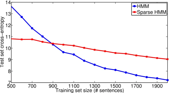
Figure 1: Test set cross-entropy of HMM vslα-regularized (sparse) HMM as a function of the number
of training sentences
5 Experiments
We test our approach on a subset of the resource management (RM) corpus (Price et al., 1993), which consists of naval commands that span approximatelyV = 1000words. First, we show that lα
regular-ization works. Figure 1 shows the estimated test set cross-entropy of an unregularized HMM and of an
lα-regularized HMM as a function of the number of training sentences. We vary the training set size from 10to2000sentences and test the models on800sentences; Figure 1 reports the average cross-entropy on brackets of training sizes –10-100,110-200, and so on. Thelα-regularized HMM requires additional tunable parameters such as the value ofα. To simplify the search on a separate300sentence development set, we make a (rather restrictive) assumption thatαfor both the transition and observation probabilities is the same, and thatαis independent of the size of the training set. Our solutions are therefore not opti-mal, but adequate to demonstrate our claims. To ensure that the cross-entropy is bounded, we smooth all estimates with add-one smoothing. For small training datasets, the unregularized HMM learns models that assign near-zero likelihood to some of the test sentences; hence, we only present results for training set sizes greater than500sentences.
Like many other model selection results, Figure 1 suggests that model sparsity is essential when train-ing datasets are small. In this example, about 900sentences are required for the unregularized HMM to outperform the sparse HMM. In the context of the theory developed in earlier sections, it was shown that test set cross-entropy is proportional toni
N, whereN is the number of training examples. In practical
settings,N is fixed; hence, the only strategy for minimizing cross-entropy is to minimizeni. Figure 1 confirms thatlαregularization successfully sparsifiesq(xi|ci), the observation probabilities of the HMM,
thereby minimizingni.
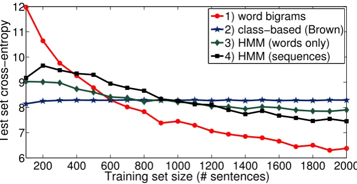
We also compare how the test set cross-entropy improves as a function of the training set size for four different models: 1) a baseline bigram model estimated over words; 2) a baseline class-based model using Brown’s algorithm (Brown et al., 1992) withK = 20clusters, learnt over the entire dataset so that it is also representative of knowledge-based approaches in which the true clusters are knowna priori; 3)lα-regularized HMM with20ergodic states; and 4) a special case of 3) in which the state transitions
are constrained to artificially formm1 = 10word clusters (10states) andm2= 5clusters that represent word bigrams (10states, where the5clusters are modeled with2left-to-right states each); therefore, the model represents an interpolation between the standard class-based model and word bigrams, but is of the exact same complexity as 2) and 3).
Figure 2 shows the estimated test set cross-entropy for each of the four models. The values of α
200 400 600 800 1000 1200 1400 1600 1800 2000 6
7 8 9 10 11 12
Training set size (# sentences)
Test set cross−entropy
1) word bigrams
2) class−based (Brown) 3) HMM (words only) 4) HMM (sequences)
Figure 2: Test set cross-entropy as a function of the number of training sentences for the four settings
from Figure 2 thatlα regularization helps even in the case of a standard class-based model, the bound
for which is already linear inV. With fewer than 100sentences, lα regularization can both learn the clusters and estimate their transitions reasonably well, and surpasses Brown for training set sizes of
N ≥ 800 sentences. Brown’s algorithm in 2) finds clusters such that pairwise mutual information terms are maximized; in 3), we not only maximize the mutual information, but we also reduce the effectiveV by ensuring that each cluster (or state) specializes and represents as few words as possible. As the number of training examples increases, estimates of class transitions indeed improve, but the class-based assumption itself becomes too restrictive. In 4), which represents an interpolated model, we see the tradeoff achieved by incorporating sequences: for small training sets, the model achieves better generalization than word bigrams, but is worse than the class-based model; and for larger training sets, the interpolated model learns better representations of high frequency events and outperforms the class-based models represented by 2) and 3).
The value ofα in 3) is0.7, whereasα in 4) is0.9; this seems counter-intuitive at first, but note that a smallerαdoes not necessarily imply sparser observation probabilities; however, it implies a heavier distribution in a Bayesian setting. A Bayesian interpretation therefore suggests that in 4), the model itself is better equipped to cope with heavy tails, whereas a more aggressiveαis required in 3).
6 Conclusion
By defining a random clustering model (a model in which there is a distribution over possible cluster assignments, e.g. an HMM), it is possible to specialize published PAC-Bayesian cross-entropy bounds to the cases of n-gram and class-based n-gram estimation. A distribution over segmentations allows derivation of a cross-entropy bound on sequence clustering algorithms, which can be made useful by sparsifying the sequence cluster observation probabilities. An efficientlα regularization technique can be used to maximize sparsity, thereby minimizing the test set cross-entropy.
Acknowledgements
References
Hirotugu Akaike. 1973. Information theory and an extension of the maximum likelihood principle. InProceedings
of the Second International Symposium on Information Theory, pages 267–281.
Sujeeth Bharadwaj, Mark Hasegawa-Johnson, , Jitendra Ajmera, Om Deshmukh, and Ashish Verma. 2013. Sparse
hidden Markov models for purer clusters. InProceedings of the IEEE International Conference on Acoustics,
Speech, and Signal Processing, pages 3098–3102.
Manuele Bicego, Marco Cristani, and Vittorio Murino. 2007. Sparseness achievement in hidden Markov models.
InProceedings of of the International Conference on Inage Analysis and Processing, pages 67–72.
Peter F. Brown, Vincent J. Della Pietra, Peter V. deSouza, Jenifer C. Lai, and Robert L. Mercer. 1992. Class-based
n-gram models of natural language. Computational Linguistics, 18(4):467–479.
Kenneth P. Burnham and David R. Anderson. 2002. Model selection and multi-model inference: a practical
information-theoretic approach. Springer.
Rick Chartrand and Valentina Staneva. 2008. Restricted isometry properties and nonconvex compressive sensing.
Inverse Problems, 24:1–14.
Stanley F. Chen and Josha Goodman. 1999. An empirical study of smoothing techniques for language modeling.
Computer Speech and Language, 13:359–394.
Stanley F. Chen. 2009. Performance prediction for exponential language models. InProceedings of NAACL HTL.
Sabine Deligne and Frederic Bimbot. 1995. Language modeling by variable length sequences: theoretical
for-mulation and evaluation of multigrams. In Proceedings of the IEEE International Conference on Acoustics,
Speech, and Signal Processing, pages 169–172.
I.J. Good. 1953. The population frequencies of species and the estimation of population parameters. Biometrica,
40(3):237–264.
Trevor Hastie, Robert Tibshirani, and Jerome Friedman. 2009. The Elements of Statistical Learning: Data Mining,
Inference, and Prediction. Springer.
Frederick Jelinek and Robert L. Mercer. 1980. Interpolated estimation of Markov source parameters from sparse
data. InProceedings of Workshop on Pattern Recognition in Practice, pages 381–397.
Raquel Justo and M. Ines Torres. 2007. Different approaches to class-based language models using word segments.
Computer Recognition Systems 2, Advances in Soft Computing, 45:421–428.
Slava M. Katz. 1987. Estimation of probabilities from sparse data for the language model component of a speech
recognizer. IEEE Transactions on Acoustics, Speech, and Signal Processing, 35(3):400–401.
Reinhard Kneser and Hermann Ney. 1995. Improved backing-off for m-gram language modeling. InProceedings
of the IEEE International Conference on Acoustics, Speech, and Signal Processing, pages 181–184.
Anastasios Kyrillidis, Stephen Becker, Volkan Cevher, and Christoph Koch. 2013. Sparse projections onto the
simplex. JMLR: Workshop and Conference Proceedings, Proceedings of the 30th International Conference on
Machine Learning, 28(2):235–243.
John Langford. 2005. Tutorial on practical prediction theory for classification. The Journal of Machine Learning
Research, 6:273–306.
Cen Li and Gautam Biswas. 1999. Clustering sequence data using hidden Markov model representation. In
Proceedings of the SPIE ’99 Conference on Data Mining and Knowledge Discovery, pages 14–21.
G.J. Lidstone. 1920. Note on the general case of the Bayes-Laplace formula for inductive ora posteriori
proba-bilities. Transactions of the Faculty of Actuaries, 8:182–192.
David J.C. Mackay and Linda C. Bauman Peto. 1995. A hierarchical Dirichlet language model.Natural Language
Engineering, 1(03):289–308.
David McAllester. 1998. Some PAC-Bayesian theorems. In COLT’ 98 Proceedings of the eleventh annual
conference on Computational Learning Theory, pages 230–234.
David McAllester. 2003. Simplified PAC-Bayesian margin bounds. InCOLT’ 03 Proceedings of the sixteenth
Mesrob I. Ohannessian and Munther A. Dahleh. 2012. Rare probability estimation under regularly varying heavy
tails. JMLR: Workshop and Conference Proceedings, 25th Annual Conference on Learning Theory, 23(21):1–
24.
Mert Pilanci, Laurent El Ghaoui, and Venkat Chandrasekaran. 2012. Recovery of sparse probability measures
via convex programming. InAdvances in Neural Information Processing Systems (NIPS), volume 25, pages
2429–2437.
P. Price, W.M. Fisher, J. Bernstein, and D.S. Pallett. 1993. Resource Management RM 2.0. InLinguistic Data
Consortium, Philadelphia.
Jose C. Principe. 2010. Information Theoretic Learning. Springer.
Lawrence R. Rabiner. 1989. A tutorial on hidden Markov models and selected applications in speech recognition.
Proceedings of the IEEE, 77(2):257–286.
Klaus Ries, Finn Dag Buo, and Alex Waibel. 1996. Class phrase models for language modeling. InICSLP ’96
Proceedings of the Fourth International Conference on Spoken Language, pages 398–401.
Ronald Rosenfeld. 1996. A maximum entropy approach to adaptive statistical language modeling. Computer,
Speech, and Language, 10:187–228.
Ronald Rosenfeld. 2000. Two decades of statistical language modeling: Where do we go from here? Proceedings
of the IEEE, 88(8).
Yevgeny Seldin and Naftali Tishby. 2010. PAC-Bayesian analysis of co-clustering and beyond. The Journal of
Machine Learning Research, 11:3595–3646.
Padhraic Smyth. 1997. Clustering sequences with hidden Markov models. InAdvances in Neural Information
Processing (NIPS), volume 9, pages 648–654.
Yee Whye Teh. 2006. A hierarchical Bayesian language model based on Pitman-Yor processes. InProceedings
of the 21st International Conference on Computational Linguistics and 44th Annual Meeting of the Association
for Computational Linguistics, pages 985–992.