Hierarchical Identity Based Encryption with Polynomially Many Levels

(1)

Hierarchical Identity Based Encryption with

Polynomially Many Levels

Craig Gentry (Stanford & IBM) and Shai Halevi? _(IBM)

Abstract. We present the first hierarchical identity based encryption (HIBE) system that has full security for more than a constant number of levels. In all prior HIBE systems in the literature, the security reductions suffered from exponential degradation in the depth of the hierarchy, so these systems were only proven fully secure for identity hierarchies of constant depth. (For deep hierarchies, previous work could only prove the weaker notion of selective-ID security.) In contrast, we offer a tight proof of security, regardless of the number of levels; hence our system is secure for polynomially many levels. Our result can very roughly be viewed as an application of Boyen’s framework for constructing HIBE systems from exponent-inversion IBE systems to a (dramatically souped-up) version of Gentry’s IBE system, which has a tight reduction. In more detail, we first describe a generic transformation from “identity based broadcast encryption with key randomization” (KR-IBBE) to a HIBE, and then con-struct KR-IBBE by modifying a recent concon-struction of IBBE of Gentry and Waters, which is itself an extension of Gentry’s IBE system. Our hardness assumption is similar to that underlying Gentry’s IBE system.

(2)

Identity-Based Encryption (IBE) is a public-key encryption scheme where one’s public key can be freely set to any value (such as one’s identity): An authority that holds a master secret key can take any arbitrary identifier and extract a secret key corresponding to this identifier. Anyone can then encrypt messages using the identifier as a public encryption key, and only the holder of the corresponding secret key can decrypt these messages. This concept was introduced by Shamir [18], a partial solution was proposed by Maurer and Yacobi [17], and the first fully functional IBE systems were described by Boneh and Franklin [5] and Cocks [11].

IBE systems can greatly simplify the public-key infrastructure for encryption solutions, but they are still not as general as one would like. Many organizations have an hierarchical structure, perhaps with one central authority, several sub-authorities and sub-sub-authorities and many individual users, each belonging to a small part of the organization tree. We would like to have a solution where each authority can delegate keys to its sub-authorities, who in turn can keep delegating keys further down the hierarchy to the users. The depth of the hierarchy can range from two or three in small organizations, up to ten or more in large ones. An IBE system that allows delegation as above is called Hierarchical Identity-Based Encryption (HIBE). In HIBE, messages are encrypted for identity-vectors, representing nodes in the identity hierarchy. This concept was introduced by Horwitz and Lynn [16], who also described a partial solution to it, and the first fully functional HIBE system was described by Gentry and Silverberg [14].

The security model for IBE and HIBE systems postulates an attacker that can adaptively make “key-reveal” queries, thereby revealing the decryption keys of identities of its choice. The required security property asserts that such an attacker still cannot break the encryption at any identity other than those for which it issued key-reveal queries. (Or in the case of HIBE, other than those for which it issued key-reveal queries or their descendants.)

For the first IBE and HIBE systems, the only known proofs of security are carried out in the random-oracle model. Canetti et al. [9] introduced a weaker notion of security called selective-ID, where the attacker must choose the identity to attack before the system parameters are chosen (but can still make adaptive key-reveal queries afterward). They proved that a variant of the Gentry-Silverberg system is secure in this model even without random oracles. Boneh and Boyen described a more efficient selective-ID HIBE [1], and later described a fully secure IBE system without a random oracle [2]. Waters [21] described what is currently the most practical adaptively-secure HIBE system without random oracles.

All currently known fully-secure HIBE systems, however, suffer from loose security reductions (whether they use random oracles or not). Specifically, they lose a multiplicative factor ofΩ(q/`)`

in the success probability, where q is the number of key-reveal queries and ` is the depth of the identity hierarchy. This means that asymptotically these reductions can only be used for hierarchies of constant depth. When considering concrete parameters, these reductions are only meaningful for hierarchies of depth two or three.

(4)

Boyen [8] proposed a framework for constructing HIBE systems from exponent-inversion IBE systems. Specifically, Boyen described some properties of pairing-based IBE systems (called parallel IBE and linear IBE), and proved that an IBE system with these properties can be transformed to HIBE with comparable security. Boyen noted that Gentry’s IBE does not quite fit within this template, and left it as an open problem to construct a HIBE system from Gentry’s IBE system. Our system, which solves this problem, does not quite fit within Boyen’s framework, yet our approach owes much to Boyen’s idea.

We construct the first fully-secure HIBE with a tight proof of security. Namely, ours is the first HIBE system that can be proven fully secure for more than a small constant number of levels. As for the systems of Gentry [13] and Gentry-Waters [15], we exhibit a tight reduction, albeit to a problem whose instances are of size linear in q+`. This solves an open problem posed in [14, 1, 2, 21, 3, 13, 8].

1.1 Loose and Tight Reductions

On a high level, the reason that most IBE systems have loose reductions is that those reductions involve the following trade-off: For each identity ID, either the simulator knows a decryption key forID, or it doesn’t. If it knows a key for ID then it does not learn anything new if the adversary choosesIDas the target identity to attack, since it could have used the decryption key to learn the same information. And if the simulator does not know a decryption key forID then it must abort if the adversary makes a key-reveal query for this identity.

The crucial difference in the security proof of Gentry’s IBE [13] is that there are many different decryption keys for each identity, and the simulator knows a small subset of these keys. Thus, the simulator can answer every key-reveal query without aborting, but still learn something when the adversary choses that identity for the challenge ciphertext. In this sense, Gentry’s IBE system fol-lows the universal hash proof paradigm of Cramer and Shoup [12]: Given a well-formed ciphertext, all the decryption keys recover the same message, but they recover different messages when the ciphertext is mal-formed (in a certain sense). The adversary is assumed to have a non-negligible advantage when the challenge ciphertext is well-formed, but has essentially no advantage (statisti-cally) when it is mal-formed; the adversary’s different behavior in these cases allows the simulator to solve the underlying decision problem. Gentry’s reduction uses an underlying hard problem that has a large problem instance (size θ(q)), to ensure that the adversary cannot use its q key-reveal queries to determine what keys the simulator possesses for the target identity. In this work we extend Gentry’s IBE system and proof to the case of a HIBE.

1.2 Constructing HIBE, Step 1: From IBBE to HIBE

(5)

is targeted at a group of identities (similarly to the identity vector in HIBE).1 However, IBBE is simpler than HIBE since decryption keys correspond only to single identities (see Section 2.2).

As a first step in constructing HIBE systems, we provide a generic transformation from IBBE to HIBE. This transformation, however, requires an “augmented IBBE system” that also has de-cryption keys corresponding to sets of identities (for decrypting ciphertexts that were encrypted for these sets). Specifically, we require akey-randomizable identity based broadcast encryption (KR-IBBE), where it is possible to generate auniformly randomdecryption keyKS for a set of identities

S from any decryption key KS0 for S0 (S (see Section 2.3). KR-IBBE is rather close to HIBE,

but a major difference is that security is defined with respect to an adversary that can only ask for decryption keys corresponding to single identities, not for sets of identities. Hence it is still simpler to design KR-IBBE and use our transformation than to design a HIBE “from scratch.”

1.3 Constructing HIBE, Step 2: Constructing KR-IBBE

Even with the simplification of KR-IBBE, our construction and its proof are still rather complex. Part of the reason for the complexity of our system and proof stems from the inherent tension between the key-randomization requirement and the Cramer-Shoup proof paradigm: On one hand, key-randomization implies in particular that one can generate a random decryption key for an identity setS from any fixed valid encryption key for the same set. On the other hand, the Cramer-Shoup paradigm require that the simulator be able to generate only a small subset of the decryption keys for the target identity set.

Our proof resolves this tension by going through an intermediate step in which we replace the full-randomization requirement with “pseudo-randomization”: Namely, from each fixed valid encryption key we can only generate a small subset of the decryption keys, but this small sub-set still looks random. In our case, the difference between “fully-random” and “pseudo-random” keys is that “fully random” keys are taken from some linear space and “pseudo-random” keys are taken from a proper subspace of this linear space. Being linear spaces of group elements, these are indistinguishable under the Decision Linear Assumption [4].

We prove the security of the “pseudo-random” system using techniques and hard problems analogous to those used by Gentry and Waters in [15], but we we need to make rather substantial modifications to the system given in [15]. (Most notably we cannot have scalars in the decryption key, so we must convert all the parameters, decryption keys, and ciphertexts into vectors of group elements.)

1.4 Organization

We begin in Section 2 below by introducing the formal definitions of HIBE, IBBE, and KR-IBBE, and then in Section 3 we describe and prove our transformation from KR-IBBE to HIBE. We then move to constructing KR-IBBE, first presenting in Section 4 the notations, tools, and assumptions on which we base out construction, and then describing the construction itself in Section 5. The proof of security is presented in Section 6.

(6)

2 HIBE and IBBE: Definitions

For simplicity, we define our encryption systems as key encapsulation mechanism (KEM). The standard transformation from KEM to encryption is ignored here.

2.1 Hierarchical Identity-Based Encryption

A HIBE system consists of the following five procedures:

Setup(λ, `) Takes as input a security parameter λand the hierarchy depth `. It outputs a public key P K and a master secret key SK. The public key implies also a key space K(P K) and an identity space ID(P K), and hierarchical identities are (ordered) tuples inID(P K)≤`_.

KeyGen(P K, SK,ID) Takes as input the public keyP K and master secret keySK, and an identity vector ID= [ID1, . . . ,IDt]∈ ID(P K)≤`. It outputs a decryption keyKID forID.

KeyDerive(P K,ID, K_ID,ID0_{) Takes as input the public key} _{P K}_{, the identity vector} _ID _and corre-sponding decryption keyK_ID, and another vectorID0_{such that}_ID _{is a prefix of}_ID0_{. It outputs} a decryption key K_ID0 forID0.

KEM(P K,ID) Takes as input the public key P K and identity vector ID. It outputs a pair (K, C), where K is the KEM key (from the key space K(P K)) andC is the ciphertext.

Decrypt(P K, C,ID, KID) Takes as input the public key P K, ciphertext C, identity vector ID and

corresponding decryption key K_ID. It outputs the corresponding KEM key K (or an error message ⊥).

We require the usual “completeness”, namely that decryption with the correct decryption key always recovers the correct KEM key. In particular, setting (P K, SK) ← Setup(λ, `) and fixing any chain of identity vectors ID1,ID2,. . .,IDt with each IDi a prefix of IDi+1, if we set KID1 ←

KeyGen(P K, SK,ID1) and thenKIDi ←KeyDerive(P K,IDi, KIDi−1,IDi) fori= 2, . . . , tand (K, C)←

KEM(P K,IDt), then we haveDecrypt(P K, C,IDt, KIDt) =K (with probability one).

Security. 2 _{Chosen-plaintext security for a HIBE system}_E_{against an adversary}_A_{is defined by the} following game between Aand a “challenger”: BothAand the challenger are given the parameters λ, `as inputs.

Setup: The challenger chooses a “challenge bit”σ∈R{0,1}, runs (P K, SK)← E.Setup(λ, `), and

gives P K to A.

Key-Reveal: The adversaryAmakes adaptive key-reveal queries to the challenger, each consisting of an identity vector ID = [ID₁, . . . ,IDt] ∈ ID(P K)≤`. If the adversary already made the

challenge query andIDis a prefix of the target identityID∗then the challenger ignores this query, and otherwise it returns to the adversary the decryption key K_ID ← E.KeyGen(P K, SK,ID). Challenge: The adversary queries the challenger with the target identity vector ID∗ = [ID∗₁, . . . ,

ID∗_t] ∈ ID(P K)≤`. If the adversary already made a challenge query before, or if it made a key-reveal query for any prefix of the target identity ID∗ then the challenger ignores this query. Otherwise the challenger sets (K1, C)← E.KEM(P K,ID∗), chooses another key at random from the key space K0 ∈R K(P K), and returns (Kσ, C) to the adversary (where σ is the challenge

bit chosen during Setup).

(7)

The adversary can make many Key-Reveal queries and one Challenge query, in whatever order. Then it halts, outputting a guessσ0 _{for the bit}_σ_{. The HIBE advantage of} _A _is

AdvHIBEE_A(λ, `) = Pr[A⇒1|σ= 1] − Pr[A⇒1|σ = 0]

Definition 1 (CPA-secure HIBE). The system E is CPA-secure if for any efficient adversary

A and any `=poly(λ) it holds thatAdvHIBEE_A(λ, `(λ)) is negligible in λ.

CCA-security is defined similarly, where the adversary can also make decryption queries (except for decrypting the target ciphertext by the target identity vector).

2.2 Identity-Based Broadcast Encryption

Identity-Based Broadcast Encryption (IBBE) is somewhat similar to HIBE, in that encryption is targeted at a group of identities (similarly to the identity vector in HIBE). However, IBBE is simpler than HIBE, since decryption keys correspond to a single identity. Formally, an IBBE system consists of the following procedures:

Setup(λ, `) Takes as input a security parameter λ and an upper bound on the group size `. It outputs a public key P K (that implies a keys space K(P K) and an identity space ID(P K)) and a master secret key SK.

KeyGen(P K, SK,ID) Takes as input the public key P K, master secret key SK, and an identity

ID∈ ID(P K). It outputs a decryption key K_ID forID.

KEM(P K, S) Takes as input the public key P K and a set of identities S ={ID1, . . . ,IDt} (with

t ≤`). It outputs a pair (K, C), where K is the KEM key (from key space K(P K)) and C is the ciphertext.

Decrypt(P K, C, S,ID, K_ID) Takes as input the public key P K, ciphertext C, identity set S =

{ID1, . . . ,IDt} (with t≤`) and the decryption key KID for some ID ∈S. It outputs the

corre-sponding KEM key K (or an error message ⊥).

We require that setting (P K, SK)←Setup(λ, `) and fixing any set of identitiesS ={ID1, . . . ,IDt}

⊂ ID(P K)≤`, if we setKID1 ←KeyGen(P K, SK, ID1) and (K, C)←KEM(P K, S), then we have

Decrypt(P K, C, S, K_ID₁) =K (with probability one).

Security. Chosen-plaintext security IBBE is similar to the corresponding definition for HIBE, with the main difference being that the adversary can only make key-reveal queries for single identities rather than identity-vectors. Let E be an IBBE system, CPA-security against an adversary A is defined by the following game between A and a “challenger”: BothA and the challenger are given the parameters λ, `as inputs.

Setup: The challenger chooses a “challenge bit”σ∈R{0,1}, runs (P K, SK)← E.Setup(λ, `), and

gives P K to A.

Key-Reveal: The adversary A makes adaptive reveal queries to the challenger. Each key-reveal query consists of an identity ID∈ ID(P K). If the adversary already made the challenge query and ID ∈ S∗ _{then the challenger ignores this query, and otherwise it returns} _K

ID ←

(8)

Challenge: The adversary queries the challenger with the target identity set S∗ = {ID∗₁, . . . ,

ID∗_t} ∈ ID(P K)≤`_{. If the adversary already made a challenge query before, or if made a}

key-reveal query for any identity ID ∈ S∗, then the challenger ignores this query. Otherwise the challenger sets (K1, C)← E.KEM(P K,ID∗), chooses another key at random from the key space K0 ∈RK(P K), and returns (Kσ, C) to the adversary (whereσ is the bit chosen during Setup).

The adversary can make many Key-Reveal queries and one Challenge query, in whatever order. Then it halts, outputting a guessσ0 for the bitσ. The IBBE advantage of Ais

AdvIBBEE_A(λ, `) = Pr[A⇒1|σ = 1] − Pr[A⇒1|σ= 0]

Definition 2 (CPA-secure IBBE). The system E is CPA-secure if for any efficient adversary

A and any `=poly(λ) it holds thatAdvHIBEE_A(λ, `(λ)) is negligible in λ.

CCA-security is defined similarly, where the adversary can also make decryption queries (except for decrypting the target ciphertext by any of the identities in the target set).

2.3 Key-Randomizable IBBE

To construct HIBE systems, we will use “augmented IBBE systems” that also have decryption keys corresponding to sets of identities: A decryption key corresponding to an identity-setS makes it possible to decrypt ciphertexts that were created with respect to this set. Formally, a Key-Randomizable Identity-Based Broadcast Encryption system (KR-IBBE) is an IBBE system with extended key generation KeyGen∗, extended decryptionDecrypt∗, and key-derivation KeyDerive, as follows:

KeyGen∗(P K, SK, S) Takes as input the public key P K, master secret key SK, and an identity set S ={ID1, . . . ,IDt} ∈ ID(P K)≤`, and outputs a decryption keyKS for S. We require that

KeyGen∗(P K, SK, S) degenerates to the original KeyGenwhen S is a singleton set S={ID}.

KeyDerive(P K, S, KS, S0) Takes as input the public key P K, an identity setS and corresponding

decryption key KS, and a supersetS0 ⊇S, and outputs a decryption key KS0 forS0.3

Decrypt∗(P K, C, S, KS) Takes as input the public key P K, an identity set S, ciphertext C that

was generated with respect to S, and the decryption keyKS forS. It outputs the KEM key K

(or an error message ⊥).

We stress thatwe make no security requirements regarding these additional procedures: the CPA-security game is still defined with respect to the original four procedures Setup,KeyGen,KEM,

Decrypt. However, we do make some functionality requirements, specifically the standard “com-pleteness” requirement onDecrypt∗ and a distribution requirement onKeyDerive.

The “completeness” requirement says that for any (P K, SK) ← Setup(λ, `) and any set of identities S, if we set KS ← KeyGen∗(P K, SK, S) and (K, C) ← KEM(P K, S), then we get

Decrypt(P K, C, S, KS) =K (with probability one).

The distribution requirement says for any (P K, SK) ← Setup(λ, `), any two sets of identi-ties S ⊆ S0_{, and any decryption key} _K

S ← KeyGen∗(P K, SK, S), the output distributions of

(9)

KeyGen∗(P K, SK, S0) andKeyDerive(P K, S, KS, S0) are almost identical. (That is, their statistical

distance is negligible in λ.)

Remark. Due to the distribution requirement above, our transformation from key-randomizable IBBE to HIBE in Section 3 results in a system where the decryption keys generated byKeyDerive

have the same distribution as the ones generated by KeyGen. Hence, the delegation issue in the HIBE definition, which was noted by Shi and Waters [19], does not apply to our system. Namely, proving security with respect to our Definition 1 implies also security with respect to the more complicated definition from [19].

3 From Key-Randomizable IBBE to HIBE

The transformation from key-randomizable IBBE to HIBE is quite straightforward: we use collision-resistant hashing to map identity-vectors to identity-sets, and then just use each of the procedures

Setup,KeyGen∗,KeyDerive,KEM,Decrypt∗ as-is.

The only non-trivial aspect of this transformation is the security reduction, since the HIBE adversary can make key-reveal queries on identity-vectors whereas the IBBE adversary can only ask for keys of “top level” single identities. We handle this difference by having the reduction algorithm generate decryption keys differently than is done in the system, which is where we need the distribution requirement of key randomization.

3.1 The Transformation

Let E = (Setup,KeyGen∗,KeyDerive,KEM,Decrypt∗) be a key-randomizable IBBE system, and we assume that we have a “matching” collision resistant hash functionHthat can hash identity-vectors into the identity space of E.4 We useH to hash identity vectors in the HIBE system into identity sets forE by setting:

H(ID1, . . . ,IDi) def= {H(ID1), H(ID1,ID2), . . . , H(ID1,ID2, . . . ,IDi)}

Note that short of finding collisions in H, we can only get H(ID1,ID2, . . . ,IDi) ∈ H(ID0) if

(ID1,ID2, . . . ,IDi) is a prefix of ID0. Then we construct a HIBE system as follows:5

HIBE.Setup(λ, `): Set (SK0, P K0) ← E.Setup(λ, `). Output SK and P K, which are the same as SK0 andP K0, except that each includes a description of the collision-resistant hash functionH as above.

HIBE.KeyGen(P K, SK,ID): Set S ←H(ID) (as above), compute KS ← E.KeyGen∗(P K0, SK0, S) and outputKID =KS.

HIBE.KeyDerive(P K,ID, K_ID,ID0): Set S ← H(ID) and S0 ←H(ID0), and note that S ⊆S0 since

ID is a prefix ofID0. Also let KS =KID, compute KS0 ← E.KeyDerive(P K₀, S, K_S, S0) and output

KID0 =K_S0.

HIBE.KEM(P K, S): Set S←H(ID), compute (K, C)← E.KEM(P K0, S) and output (K, C).

HIBE.Decrypt(P K, C,ID, K_ID): SetS←H(ID),KS=KID, and returnE.Decrypt∗(P K0, C, S, KS). 4_{In our IBBE system from Section 5, the identity space is}_Z

q for a large primeq, so “matching” a hash function is not a problem.

(10)

3.2 A Tight Reduction

Theorem 1. Suppose that there exists a HIBE adversary A that breaks CPA security (resp. CCA security) of the HIBE construction with advantage . Then, there exists an IBBE adversary B

and a collision finder B0_{, both running in about the same time as} _A_{, such that} _B0 _{finds a hash} function collision with some probability 0 _and _B _{breaks the CPA security (resp. CCA security) of} the underlying KR-IBBE system E with advantage −0.

Proof. B attacks receives a public key P K0 from the challenger. It sets P K to be P K0 with the hash functionH, and sends P K to A.

When A requests a HIBE key for identity vector ID = (ID₁, . . . ,IDt), B sets S ← H(ID) =

{ID0₁, . . . ,ID0_t} (with ID_i0 = H(ID1, . . . ,IDi)). B asks the IBBE challenger for the decryption key

K_ID0

t, corresponding to the last identity ID 0

t=H(ID1, . . . ,IDt). Ift= 1, it forward KIDt to A; else,

it returns to Athe decryption key KID =KS ← E.KeyDerive(P K0,{ID0t}, KID0 t, S).

In the CCA case, B handles decryption queries in the obvious way (forwarding, after replacing

ID withS =H(ID)).

When A asks for the challenge ciphertext with respect to identity vectorID∗ = (ID∗₁, . . . ,ID∗_t),

B again sets S∗ ← H(ID∗), makes a challenge query to the IBBE challenger with target identity-set S∗ (unless there is a hash collision, see below), and return to A whatever it got back from its challenger.

Finally, whenAhalts with a guess bitσ0_{, then}_B_{forward the same bit}_σ0 _{to its IBBE challenger.}

The collision finderB0proceeds just likeB, except that it saves all the queries thatAmakes and looks for collisions of the formH(ID₁, . . . ,IDi) =H(ID01, . . . ,ID0j) (where (ID1, . . . ,IDi), (ID01, . . . ,ID0j)

are prefixes of queries made byA). Denote by0 _{the probability that}_B0 _{finds any such collision.}

We claim that B’s simulation appears to A to be perfectly distributed as long as no collisions occur. This is true, because the distribution requirement on E.KeyDerive implies that the HIBE key thatB gets for identity vectorID= (ID1, . . . ,IDt) has almost the same distribution, regardless

of whether it is obtained by KeyGen (as it would in an actual attack on the HIBE system) or by

KeyDerivefrom {ID0_t}(as computed by B). Hence, the advantage of Bis at least −0. ut

Remark.Observe that the proof above only uses the fact thatKeyDerivehas the same distribution as

KeyGenwhen it starts from a singleton keyK_{ID0

t}. This is because we are using here the simplistic

security definition for HIBE that does not address the delegation issue. To prove the more elaborate notion of Shi and Waters [19] we would need to use the full power of the distribution requirement.

4 Notations and Preliminaries

We now introduce notations and hardness assumption that are used to establish our key-randomizable IBBE in Section 5. We denote the set of integers frommton(inclusive) by [m, n]. We denote poly-nomials by uppercase letters in San-serif font, for exampleP,Q,T, etc. We use the following simple fact about polynomials:

(11)

4.1 Bilinear maps and our additive notations

Our system (and its security proof) make heavy use of linear algebra. We therefore use additive notations for all the groups that are involved in the system. Specifically, we use Zq — the field of

integers modulo a primeq — as our base scalar field, and we have two order-q groups that we call thesource group Gand target group GT, both of which can be viewed as vector spaces over Zq.

Throughout the writeup we denote elements of the source group with a hat over lowercase letters (e.g., ˆa,ˆb, etc.) and elements of the target group with a tilde (˜a,˜b, etc.). Scalars will be denoted with no decorations (e.g.,a, b, and sometimes also τ, ρ, etc.)

We will make use of an efficiently computable bilinear map from the source group to the target group e:G×G→ GT, such that for any two source-group elements ˆa,ˆb∈Gand any two scalars

u, v ∈Zq it holds that

e(u·a, vˆ ·ˆb) =uv·e(ˆa,ˆb)

The neutral elements in the groups G,GT are denoted by ˆ0, ˜0, respectively. We also denote by ˆ1

some fixed generator in G, which we consider to be part of the description of G. We require that the mapping e is non-trivial, which means that e(ˆ1,ˆ1) is a generator in GT, and we denote this

generator by ˜1 =e(ˆ1,ˆ1).

More generally, for a scalar a ∈ Zq, we denote the source-group element a·ˆ1 by ˆa, and the

target-group element a·˜1 =e(â,ˆ1) by ã. Conversely, for an element â∈G, its discrete-logarithm based ˆ1 is denoted a∈Zq. (Readers who are used to multiplicative notations may find it easier to

think of â, ã as denoting “a in the exponent” in the appropriate groups.) Note also that in these notations, the discrete-logarithm of âwith respect to ˆb is just their “ratio” â/ˆb, which is a scalar.

With these notations, we usually omit the mapealtogether, and simply denote it as a “product” of two source-group elements:

ˆ

a·ˆb def= e(ˆa,ˆb) = ˜ab ∈ GT

Note that the bi-linearity ofe looks in these notations just like the natural commutative property of products ˆua·vbˆ =uv·ab˜.

Below we slightly abuse notations to denote “powers of group elements”: If ˆais a group element with discrete-logarithm a, then we denote ˆai def₌ _ai_·_ˆ_{1 and we call ˆ}_ai _the _i_{’th power of ˆ}_a_.6

Vectors and matrices. We extend our notations to vectors and matrices: A vector of scalars is denoted with no decoration a = [a1, a2, . . . , an], a vector of source-group elements denoted

with a hat, â = [â1,â2, . . . ,ân], and a vector of source-group elements denoted with a tilde ã =

[ã1,ã2, . . . ,ãn]. All these vectors are considered row vectors.

Matrices are denoted by uppercase letters, e.g., A for a matrix of scalars, ˆA for a matrix of source-group elements, and ˜A for a matrix of target-group elements. We denote the i’th row of A by Ai, the sub-matrix consisting of rows i, j, k by Ai,j,k, and the sub-matrix consisting of rows i

through j is denotedAi..j. As usual, the transposed matrix of Ais denoted At.

We denote by span(x,y,z) the linear space that is spanned by the vectors x,y,z, and also use the same notation to denote the uniform distribution over this space. For example, we use ˆ

u←wˆ +span( ˆA1,2,4) as a shorthand for the process of choosing three random scalarsa, b, c∈RZp

and setting ˆu←wˆ +aAˆ1+bAˆ2+cAˆ4.

(12)

Inner and outer-products.For vectors a,b, we denote their inner product byha,bidef= P_iaibi.

We use the same inner-product notations also for vectors of source-group elements, namely:

D

a,ˆbE=Dˆb,aEdef= X

i

aiˆbi=ha,bi·ˆ1∈G, and

D ˆ

a,ˆbEdef= X

i

ˆ aiˆbi =

X

i

e(ˆai,ˆbi) =ha,bi·˜1∈GT

It is easy to check that all the commutative, associative, and distributive properties of inner products hold for both scalars and group elements.

Similar notations apply to matrix multiplication, for either scalar matrices or group-element matrices. For example, if A is an `×m scalar matrix and ˆB is an m×n matrix of source-group elements, then ABˆ ∈G[`×n] is a matrix of source-group elements whose i, j element is the inner product of thei’th row ofAby thej’th column of ˆB. We also usea×bto denote the outer product of two vectors. Namely, the outer product of the m-vectora by then-vectorbis them×nmatrix obtained as the matrix product of the m×1 matrixatby the 1×nmatrix b. The same notation applies to vectors of group elements.

Linear algebra. All the standard concepts from linear algebra behave just the same with either scalars or group elements. For example, if Â∈G[n×n] is a square matrix of source-group elements and A is the matrix of the discrete logarithm of all the elements in Â (with respect to the fixed generator ˆ1), then the inverse of Â is Â−1 =A−1·ˆ1. (Equivalently, the inverse of Â is the unique matrix ˆB such that Â·Bˆ = ˜I.) Similarly, the rank of a scalar matrix is defined as usual, and the rank of a matrix of group elements is defined as the rank of their discrete-logarithm matrix.

4.2 The BDHE-Set assumption

The BDHE-Set assumption (used also in [15]) is a parameterized generalization of the t-BDHI problem from [1].7 Recall that at-BDHI adversary is given t+ 1 powers of a random source-group element, ˆ1,a,ˆ aˆ2, . . .ˆat_{, and it needs to distinguish the target-group element ˜}_a−1 _{from random.}

An instance of the BDHE-Set assumption is parameterized by a set of integers S ⊂ Z and another “target integer” m. The BDHE-Set adversary is given some powers of a random source-group element, {ˆai _: _i_{∈ S}}_{, and it (roughly) needs to distinguish the target-group element ˜}_am

from random. Denoting S+qS def= {i+jmodλ(q) :i, j∈ S}, where λ(q) is the order of elements

modulo q, it is easy to see that if G is an order-q bilinear-map group and m ∈ S+qS then the

problem is easy: Just choose somei, j ∈ S such that i+j=mmodλ(q) and compute the bilinear map

e(âi,âj) = âi·âj = ãi+j = ãm

However, whenm /∈ S+qS then there does not seem to be an easy way of distinguishing ˜am from

random given the source-group elements {ˆai _: _i_{∈ S}}_{. The formal BDHE-Set assumption below}

is somewhat stronger, however, giving the adversary not the target group element ˜am _{itself, but}

rather two random source group elements whose product is ˜am_{. Even so, this may be a reasonable}

assumption to make.

Definition 3 (Decision BDHE-Set). Fix a prime number q, a set of integers S and another integer m /∈ S +qS. Also fix two order-q groups G and GT, admitting a non-trivial, efficiently computable bilinear map e:G×G→G_T.

(13)

The (S, m)-BDHE-Set problem with respect to G and GT consists of the following experiment: Choose at random a scalara∈RZ∗q and a bitσ∈R{0,1}. Ifσ = 0 then choose two random scalars

z1, z2 ∈R Z∗q, and if σ = 1 then choose a random scalar z1 ∈R Z∗q and set z2 ← a/z1 modq. The

BDHE-Set adversary gets as input aˆi ₌_ai_·_ˆ₁ _{for all} _i_{∈ S} _{and also} _z_ˆ

1,zˆ2, and its goal is to guess

the bit σ. The advantage of an adversary A is defined as

AdvBDHES,m_A (G,GT) def= Pr

a, z1 ∈RZ∗q, z2 ← a z1

, A {ˆai :i∈ S},zˆ1,zˆ2⇒1

− Pra, z1, z2 ∈RZ∗q, A {ˆai :i∈ S},zˆ1,zˆ2⇒1

Informally, the asymptotic Decision BDHE-Set assumption states that for anym /∈ S+S and a large enough primeq, efficient adversaries (that work in time poly(|S|,logq) only have insignificant advantage in the experiment from above. Making this formal is rather straightforward (though getting the quantification right takes some care).

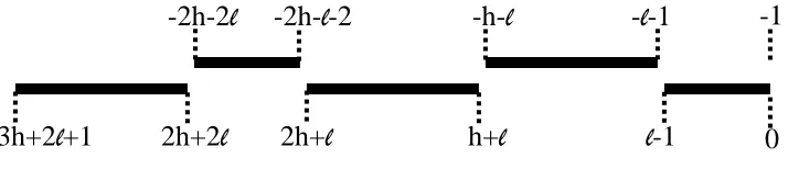
Jumping ahead, for our system we use the assumption above with the target integer m =−1 and the setS defined as:

S = [−2h−2`, −2h−`−2] ∪ [−h−`, −`−1] (1)

∪[0, `−1] ∪ [h+`,2h+`] ∪ [2h+ 2`,3h+ 2`+ 1]

where`is the depth of the identity-hierarchy of the system andhis some other parameter. (Specif-ically, if q∗ is a bound on the number of queries then h = q∗ +`+ 2.) This set S is depicted in Figure 1, which makes it clear that S+S indeed does not include the target integerm=−1.

-2h-2

1 -2h-

1 -2

-h-

1 -

1 -1

-1

0

1 _-1

2h+

1 h+

1 2h+2

1 3h+2

1 +1

Fig. 1.A graphic depiction of the setS_{, “folded” around the point}_m/_{2 =}−₁_/_2.

4.3 The Linear Assumption

The decision linear assumption, first defined in [4], states (in our additive notations) that given the six source group elements ˆa,ˆb,ˆc, ˆd,ˆe, ˆf, it is hard to distinguish the case where these elements are completely random from the case where they are chosen at random subject to the condition

ˆ

f /ˆc= ˆe/ˆb+ ˆd/ˆa. (I.e., the discrete logarithm offrelative tocis the sum of the discrete logarithm ofe relative toband the discrete logarithm ofdrelative toa.) Note that this assumption is equivalent to saying that given the matrix of group elements

M =



 ˆ aˆ0 ˆc ˆ 0 ˆb ˆc

ˆ deˆfˆ



(14)

it is hard to decide if this matrix is invertible or has rank two. In this work we use a slightly weaker variant of this assumption, only assuming that given a 3×3 matrix of source-group elements, it is hard to distinguish the case where this is a random invertible matrix from the case where it is a random rank-two matrix. (This weaker assumption is implied both by the standard linear assumption and by our BDHE-Set assumption, but we make it a separate assumption just to make the exposition of our security-proof easier.)

5 A Key-Randomizable IBBE system

Our system operates in prime-order bilinear-map groups. In the description below we assume that these order-q groups are fixed “once and for all” and everyone knows their description. (An alter-native description will include the group-generation as part of the Setup procedure.) We also fix the hierarchy-depth of the system to some integer`.

The identity space of the system is the scalar field Zq, except that we have`“forbidden

identi-ties” within this range: `−1 of them are arbitrary (and we set them to be 0,1, . . . , `−2), and the last one is a random scalar athat is chosen duringSetup (see below).

Setup: Choose three random scalars a, b, s ∈ Zq and a random invertible matrix A ∈ G[7×7],

and set ˆB = ( ˆA−1₎t_{. We note that the system only uses the top four rows of ˆ}_A _{and five rows}

of ˆB. The seventh dimension is only used in the security proof. Below we denote by ai the vector

ai def= [1 a a2. . . ai].

– The master secret key is SK = ( ˆB1..6, s,a`).

– The public key consists of three parts, P K = (P K1, P K2, P K3) with P K1 consisting of a target-group element that is used to compute the KEM key, P K2 consisting of multiples of the rows of ˆAthat are used to compute the ciphertext, andP K3 consisting of multiples of the rows of ˆB that are used only for key randomization. Specifically we have

P K1 = a`−1s˜ (2)

P K2 =

{aiA1ˆ : i= 0, . . . , `}

| {z }

a`×Aˆ1

, sA2,ˆ {aiA3ˆ : i= 0, . . . , `−1}

| {z }

a`−1×Aˆ3

, A4ˆ

P K3 =

bsBˆ1, absBˆ1, Bˆ5, Bˆ6,

{aibBˆ1 : i= 0, . . . , `}

| {z }

b(a`×Bˆ1)

, {aibBˆ2 : i= 0, . . . , `}

| {z }

b(a`×Bˆ2)

, {aibBˆ3: i= 0, . . . , `+ 1}

| {z }

b(a`+1×Bˆ3)

(15)

KeyGen (P K, SK,ID): Choose a key of 3`−3 7-dimensional vectors of source-group elements as follows: Pick at randomr_ID ∈Zq and set ˆKID= (ûID,VÎD,WÎD,XÎD,yÎD), where

ˆ

u_ID= s−rID

a−IDBˆ1, (3)

ˆ

V_ID=r_ID(a`−2×Bˆ1)

={r_IDaiBˆ1 : i= 0, . . . , `−2}

,

ˆ

W_ID=a`−1×Bˆ2

={aiBˆ2 : i= 0, . . . , `−1}

,

ˆ

X_ID=r_ID(a`−2×Bˆ3)

={r_IDaiBˆ3 : i= 0, . . . , `−2}

,

ˆ

y_ID=r_IDa`−1Bˆ3+span( ˆB5,6)

Note that the ˆW_ID component is the same for all identities (so it really belongs in the public key). It is included in the secret key only for the purpose of the key-randomization procedure below.

KEM (P K, S): If|S|< `then add toS the first`−|S|of the “forbidden identities” 0,1, .... Denote the resulting `identities by{ID1,ID2, . . . ,ID`}.

– Set the monic degree-` polynomialP(x)def= Q`_i₌₁(x−IDi), let p0, . . . , p` be the coefficients of P

and denote pdef= [p0 . . . p`] (soP(a) =hp,a`i).

– Choose at random f0, . . . , f`−1 ∈ Zq and denotef def= [f0 f1 . . . f`−1] and F(x) def= Pi`−=01fixi.

Make sure that F(IDi)6= 0 for alli= 1, . . . , `(otherwise re-choose Funtil this condition holds).

– Choose a random scalar t∈Zq.

– Output the ciphertext containing the polynomial F and the vector

ˆ c=t

P(a) ˆA1 | {z }

p(a`×Aˆ1)

+ sAˆ2 + F(a) ˆA3 | {z }

f(a`−1×Aˆ3)

+span( ˆA4) (4)

The implied KEM key is the target-group element ˜k=t·P K1=a`−1ts˜.

Remark. Note that the ciphertext include seven source group elements and ` scalars (to specify

F). The ciphertext size can be reduced in a particular way, so that when encrypting to a set S of size m < `we only have m scalars in the ciphertext: Instead of choosingF completely at random, we impose the condition that F(ID) = 1 for each of the “forbidden identities” that were added to S. This way, the encryptor can specify F using only the m scalars F(IDi) for all IDi ∈S. This

optimization requires a small change to the proof of security, see remark at the end of Section 6. We also note that we can get a constant-size ciphertext by moving to the random-oracle model: the encryptor just sends some nonce, and F is determined by applying the random oracle to this nonce.

Decrypt (P K,(F,ˆc), S,ID,KˆID), where ID ∈ S. If |S|< ` then add to S the first `− |S| of the

“forbidden identities” 0,1, .... Denote the resulting`identities by{ID1,ID2, . . . ,ID`}. Parse the key

as ˆK_ID= (ˆu_ID,Vˆ_ID,Wˆ_ID,Xˆ_ID,yˆ_ID), recalculate the monic `-degree polynomialP(x) =Q`_i₌₁(x−IDi),

(16)

– SetQ_ID(x)def= P(x)

x−ID and Q

0

ID(x) =QID(x)−a

`−1_{. (That is,}_Q0 _{is the polynomial}_Q_{without the}

top coefficient of 1·x`−1_{.) Denote the coefficient vector of} _Q0

ID byq0ID= [q0 q1 . . . q`−2].

– Set G_ID(x)def= F(x)−F(ID)

x−ID and denote the coefficient vector of GID by gID= [g0 g1 . . . g`−2].

– Set

ˆ

d_ID =uˆ_ID−q0

ID·WˆID−

g_ID·Vˆ_ID−q0

ID·XˆID−yˆID

F(ID) (5)

Finally, recover the KEM key as ˜k=Dˆc,dˆ_IDE.

5.1 Correctness

To argue correctness, we can rewrite

ˆ

d_ID = s−rID

a−IDBˆ1

| {z }

ˆ u_ID

− q0

ID·(a`−2×Bˆ2

| {z } ˆ

W_ID

)

−

g_ID·(r_IDa`−2×Bˆ1

| {z }

ˆ

V_ID

)−q0

ID·(rIDa`−2×Bˆ3

| {z }

ˆ

X_ID

)−(r_IDa`−1Bˆ3+span( ˆB5,6))

| {z }

ˆ y_ID

/F(ID)

= s−rID

a−IDB1ˆ −

q0

ID,a`−2

_ˆ B2

− rID F(ID)

hg_ID,a`−2iBˆ1−q0ID,a`−2

+a`−1Bˆ3−span( ˆB5,6)

=

s−r_ID a−ID −

r_IDG_ID(a)

F(ID)

ˆ

B1−(QID(a)−a

`−1_{) ˆ}_B 2+

r_ID

F(ID)

Q_ID(a) ˆB3+span( ˆB5,6)

Further developing the coefficient of ˆB1 we get

s−r_ID a−ID −

r_IDG_ID(a)

F(ID)

= F(ID)(s−rID)−rIDGID(a)(a−ID) F(ID)(a−ID)

= F(ID)(s−rID)−rID(F(a)−F(ID)) F(ID)(a−ID)

= s·F(ID)−rID·F(a) F(ID)(a−ID)

Examining the inner-product of cˆ with dˆ_ID, we use the fact that DAˆi,Bˆj

E

is either 0 (when

i6=j) or ˜1 (wheni=j). Hence the span’s of ˆA4 and of ˆB5,6 drop out completely, and we are left with the product of the matching coefficients only:

D ˆ c,dˆ_ID

E =

tP(a)s·F(ID)−rID·F(a) F(ID)(a−ID)

| {z }

coefficients of ˆA1,Bˆ1

−ts(Q_ID(a)−a`−1)

| {z }

+tF(a) rID

F(ID)QID(a)

| {z }

(17)

The first term in the parenthesis above can be simplified usingQ_ID(a) =P(a)/(a−ID), so we get

D ˆ

c,dˆ_IDE = t

Q_ID(a)s·F(ID)−rID·F(a)

F(ID) −s(QID(a)−a

`−1_{) +}_F₍_a₎ rID

F(ID)QID(a)

·˜1

= t

Q_ID(a)s−rIDQID(a)F(a)

F(ID) −QID(a)s+a

`−1_s₊rIDQID(a)F(a) F(ID)

·˜1

= a`−1ts·˜1 = ˜k

u t

5.2 Key randomization

Our key-randomization follows Boyen’s idea from [8], where the key for identity-setS ={ID1, . . . ,IDm}

consists ofm“shifted versions” of the keys, r0

ID1

ˆ

K_ID₁,. . .,r0

IDn

ˆ

K_IDm, such thatP_ir0

IDi = 1 (mod q).

Namely, the augmented procedure KeyGen∗(P K, SK, S) uses the same KeyGen procedure from abovem times to get

ˆ

K_IDi ←KeyGen(P K, SK,IDi)

Then for i= 1. . . m it chooses r0

IDi ∈Zq at random subject to the constraint

P

irID0 i = 1 (modq),

and outputs the secret key

ˆ

KS = [r_ID0 1

ˆ

KID1, . . . , r 0

IDm

ˆ KIDm]

wherer_ID0

i

ˆ

KIDi means multiplying all the elements in ˆKIDi by the scalarr0_ID

i. Below we call ˆKIDi the singleton key corresponding toIDi, and r_ID0

i

ˆ

K_IDi is the shifted singleton key forIDi.8 Note that for

the special casem= 1, we haver0_ID= 1, so KeyGen∗ degenerates to the original KeyGen.

Extended decryption. The extended decryption procedureDecrypt∗ is given a ciphertext (F,ˆc) together with a set of identities S ={ID1, . . . ,IDm} (m ≤`) and a matching decryption key ˆKS.

It parses the decryption key as ˆKS = [ ˆK_ID0 ₁, . . . ,Kˆ_IDm0 ] where the ˆK_IDi0 ’s are shifted singleton keys.

Namely we have ˆK_IDi0 = r0_ID

i

ˆ

KIDi where the ˆKIDi’s are singleton keys and PirID0 i = 1 (mod q).

Then we use each shifted singleton key to produce ˆd0_IDi just as in Eq. (5), sets ˆdS =Pidˆ0IDi, and

recover ˜k=Dˆc,ˆdS

E .

Correctness holds since the decryption process in linear: Denote by ˆd_IDi the vector that would have been obtained from the singleton key ˆK_IDiusing Eq. (5). Then on one hand decryption is linear so we have ˆd0

IDi =r0_ID_idˆ0IDi. On the other hand by correctness of the basic decryption procedure

we know thatDc,ˆ dˆ_IDi E

= ˜k. We therefore get

D ˆ c,dˆS

E

= X

i

D ˆ

c, dˆ0_IDiE = X

i

D ˆ c, r0

IDi

ˆ

d_IDiE = X

i

r0

IDi

D ˆ

c,dˆ_IDiE = X

i

r0

IDi

˜ k = ˜k

8_{Note that ˆ}_K

(18)

Key derivation. Key-derivation uses Boyen’s idea of reciprocal keys [8]. Namely, given the public key and any two identities ID1 andID2, anyone can compute a pair of shifted singleton keysδKˆID1

and δKˆID2 for the same (unknown) scalar factor δ. The procedure for generating these reciprocal

keys (which is used as a subroutine for key derivation) is as follows:

ReciprocalKeys (P K,ID1,ID2): recall that the public keyP Kdepends on the unknown scalarsa, b, s (among other things).

– Choose at random z∈Zq. The shifted singleton keys δKˆIDi will have δ=bz(a−ID1)(a−ID2). – Choose at randomr1, r2 ∈Zq (which will play the role ofrID1 and rID2 in the reciprocal keys).

– ComputeδKˆ_ID₁ as

δ· s−r1

a−ID1 ˆ

B1 = (abs−bsID2−abr1+br1ID2)zBˆ1

δ·r1(a`−2×Bˆ1) = br1z(ai+2−ai+1(ID1+ID2) +aiID1ID2) ˆB1, i= 0, . . . , `−2 δ·(a`−2×Bˆ2) = bz(ai+2−ai+1(ID1+ID2) +aiID1ID2) ˆB2, i= 0, . . . , `−2 δ·r1(a`−2×Bˆ3) = br1z(ai+2−ai+1(ID1+ID2) +aiID1ID2) ˆB3, i= 0, . . . , `−2

δ·r1a`−1B3ˆ +span( ˆB5,6)

= br1z(a`+1−a`(ID1+ID2) +a`−1ID1ID2) ˆB3+span( ˆB5,6)

and similarly forδKˆID2 (usingr2 instead ofr1 and swapping the roles of ID1,ID2). Notice that

the terms ai_b_B_ˆ

j fori∈[0, `],j = 1,2,3, as well asbsBˆ1,absBˆ1, a`+1bBˆ3, and ˆB5,6, are all part of the P K3 component of the public key.

From the description above it is clear that whenID₁,ID₂ 6=a, thenReciprocalKeysindeed returns the correct distribution, namely two shifted singleton keys δKˆ_ID₁,δKˆ_ID₂ where each ˆK_ID is drawn from the same distribution as the singleton keys for ID in KeyGen and δ is chosen at random in Zq (and independently of ˆKID1,KˆID2).

KeyDerive (P K, S,KˆS, S0) (where S0 = {ID1, . . . ,IDm} and S ⊆ S0). Assume (w.l.o.g.) that S

consists of the first n identities in S0_{, namely} _S ₌ _{ID

1, . . . ,IDn} with n ≤ m. Denote ˆKS =

{Kˆ0

ID1, . . . ,Kˆ 0

IDn}, where ˆKIDi0 is the shifted singleton key forIDi (consisting of 3`−3 7-dimensional

vectors of source-group elements).

For i = 1, . . . , m, run the ReciprocalKeys procedure from above with identities IDi and IDi+1 (indexing modm) to get two shifted singleton keys for theseID’s, which we denote by ˆL_IDi,Mˆ_IDi₊₁, respectively. Namely, set

( ˆLIDi,MˆIDi+1)←ReciprocalKeys(P K,IDi,IDi+1)

Then fori∈[1, n] set ˆK_IDi∗ = ˆK_IDi0 + ˆL_IDi−Mˆ_IDi, and fori∈[n+1, m] set ˆK_IDi∗ = ˆL_IDi−Mˆ_IDi (where addition and subtraction is element-wise). The new key is ˆKS= [ ˆK_ID∗ ₁, . . . ,Kˆ_IDm∗ ]. In Lemma 2 below

we show that this KeyDerive procedure induces almost the same distribution as KeyGen over the decryption key ˆKS0.

(19)

Proof. Observe that every 7-vector in a singleton key ˆK_IDcorresponding to identityID(as computed by KeyGen) is of the form

(expr(a, s,ID) +r_IDexpr0(a, s,ID))·Bˆk

where r_ID is the scalar that was chosen for this singleton key, ˆBk is one specific row of the matrix

ˆ

B, andexpr(a, s,ID),expr0(a, s,ID) are two fixed scalar-valued expressions that depend only on the scalars a, s from the master secret key and on the identity ID. (Note that either expr(a, s,ID) or

expr0(a, s,ID) can be zero, but not both.)

Considering the same vector in all the shifted singleton keys in ˆKS, we have a collection of n

vectors, ˆx1, . . . ,xˆn, where

ˆ xi=r_ID0

i(expr(a, s,IDi) +rIDiexpr

0₍_{a, s,}_ID i))·Bˆk

where the scalars r0

IDi satisfy

P

irID0 i = 1. For notational convenience, fori∈[n+ 1, m] we denote

r_ID

i =r 0

IDi = 0 and ˆxi = ˆ0 (so we still have ˆxi’s of the right format with

P

ir0IDi = 1, even when we

consider all melements).

Similarly considering the same vector in all the shifted singleton keys that are generated by

ReciprocalKeys, we have vectors ˆy₁. . .yˆ_m (from the ˆL_IDi’s) and ˆz1. . .zˆm (from the ˆMIDi’s) of the

form

ˆ

y_i = δi(expr(a, s,IDi) +ρi expr0(a, s,IDi))·Bˆk

and ˆzi =δi−1(expr(a, s,IDi) +τi expr0(a, s,IDi))·Bˆk

where all the scalars δi, ρi, τi,i= 1. . . m, are chosen at random in Zq (and indexing is mod m, so

δ0 =δm). Hence the corresponding element in the shifted singleton key ˆK_IDi∗ is

ˆ

xi+ ˆyi−zˆi =

(r_ID0

i+δi−δi−1)expr(a, s,IDi) + (r 0

IDirIDi +δiρi−δi−1τi)expr

0₍_{a, s,}_ID i)

ˆ Bk

Assuming that r_ID0

i+δi−δi−16= 0, we can denote

r_ID∗∗

i

def = r0_ID

i +δi−δi−1 and r ∗

IDi

def

= r

0

IDirIDi +δiρi−δi−1τi

r0

IDi +δi−δi−1

and then we have

ˆ

xi+ ˆyi−zˆi = r∗∗_ID

i(expr(a, s,IDi) +r ∗

IDiexpr

0₍_{a, s,}_ID i)) ˆBk

which is of the right form, and indeed the scalars r∗∗

IDi satisfy m

X

i=1 r∗∗

IDi =

m

X

i=1 r0

IDi +

m

X

i=1 δi−

m

X

i=1

δi−1 =

m

X

i=1 r0

IDi = 1

Since theδi’s are random and independent then ther_ID∗∗

i’s are also random and independent subject

to the constraint that their sum is one. Finally, assuming that none of the r_ID∗∗

i’s is zero and also

none of the δi’s are zero (which happens with probability at least 1−O(m/q)) then all the r_ID∗ i’s

(20)

6 Security Proof

We now prove security of our system based on the decision BDHE-Set and linear assumptions. On a very high level, the proof follows the hash-proof approach: The simulator (in Proposition 3 below) will generate the challenge ciphertext so that this is either a valid ciphertext or an invalid one, depending on whether the input of the simulator is a YES instance or a NO instance of the decision BDHE-Set problem. In our case, a valid ciphertext is spanned by the rows ˆA1,2,3,4, and an invalid ciphertext also has a component of ˆA7. The secret keys will have a random ˆB7 component in them, so an invalid ciphertext will be decrypted to a random KEM key (while a valid ciphertext will always be decrypted to the “right KEM key”).

We now proceed to describe the actual proof, consisting of four games: roughly, Game 0 is the actual interaction of the adversary with our system, in Game 1 we use decryption rather than encryption to compute the KEM key corresponding to the challenge ciphertext, in Game 2 we add a component of ˆB7 to the secret keys, and in Game 3 we add a component of ˆA7 to the challenge ciphertext vector. Fix an adversaryA, and we denote the event that the adversary wins game iby Wi, and will show that Pr[Wi]≈Pr[Wi+1] and that Pr[W3] = 1₂.

Game 0 is the semantic-security game from Definition 2, so Pr[W0]−1₂ is half the CPA-advantage of the adversary against our system. We describe this game for self-containment: The challenger begins by choosing a random invertible 7×7 scalar matrix Â ∈ G[7×7] and random scalars a, b, s ∈Zq, and sets ˆB = ( Â−1)t. From a, b, s,Aˆ1..4 and ˆB1..6, the challenger computes the secret key SK = ( ˆB1..6, s,â`) and the public key P K = (P K1, P K2, P K3) as in Eq. (2). (Note that the challenger never uses the last three rows of Âin the public key or anywhere else. We will use that fact in the proof of Proposition 1 below.)

Then the challenger send P K to the IBBE adversary. When the adversary makes a key-reveal query for identity ID, the challenger runs the procedure KeyGen(SK,ID) from Section 5 to get

ˆ

K_ID= (ˆu_ID,Vˆ_ID,Wˆ_ID,Xˆ_ID,yˆ_ID). When the adversary makes a challenge ciphertext query for identity-set S∗ _{then the challenger runs the procedure}_KEM₍_{P K, S}∗_{) to get the KEM key and ciphertext}

(˜k1,(F,cˆ)) =KEM(P K, S∗)

It also picks another random target-group element ˜k0 and a random bit σ, and returns to the adversary ˜kσ and (F,cˆ). (Since the KEM procedure always “pads” the set S to size `, below we

assume w.l.o.g. that the target set S given by the adversary is always of size exactly `.) The adversary can make more key-reveal queries, and eventually it halts with output bit σ0_{. It wins}

the game if it never made key-reveal query on any of the identities ID∗_i ∈ S∗ and yet it guessed correctly σ0 =σ.

Game 1 proceeds like Game 0, except that we change the KEM procedure that the challenger uses to produce the challenge ciphertext and KEM key. Specifically, the challenger still uses the KEM procedure to get the challenge ciphertext (F,cˆ), but uses the decryption procedure to derive the KEM key. Namely, instead of deriving the corresponding KEM key as ˜k1 = t·a`−1s˜g (as done in the KEM procedure) it uses KeyGen to derive a key ˆK_ID∗

1 and computes the KEM key as

˜

(21)

Clearly, since decryption always recovers the correct KEM key then the same value of ˜k1 is returned in either Game 0 or Game 1. These games are therefore identical and we have Pr[W0] = Pr[W1].

Game 2 proceeds like Game 1, except that all the vectors yˆ_ID in the secret keys have a ˆB7 component in them. Specifically, the challenger sets

ˆ

y_ID = r_ID(a`−1Bˆ3+ ˆB7) +span( ˆB5,6) (6)

where ˆB7 is the last row of ˆB (that so far was not used anywhere in the system).

This alternative procedure for generating yˆ_ID is used both in answering key-reveal queries and when deriving the key ˆK_ID∗

1 in the alternative KEM procedure that is used for answering the

challenge ciphertext query. We now prove that under the decision linear assumption, the attacker cannot distinguish Game 1 from Game 2.

Proposition 1. There is an adversary B for the linear problem that has advantage of at least

Pr[W2]−Pr[W1]−1_q.

Proof. The linear adversary B gets a 3×3 matrix of source-group elements ˆM ∈G[3×3] and it needs to decide if ˆM is an invertible matrix or a rank-two matrix. B chooses a random invertible matrix A ∈Zq[7×7] and computes B = (A−1)t. Let B5,6,7 be the 3×7 matrix consisting of the last three rows of B0. It sets ˆA=A·ˆ1 and ˆB =B·ˆ1, and then replaces the last three rows ˆB5,6,7 with ˆB0

5,6,7 = ˆM ·B5,6,7. We let ˆB0 be the matrix with top four rows ˆB1,2,3,4 and bottom three rows ˆB0

5,6,7. Next Bchooses at random also a, b, sand proceeds just like the challenger in Game 2 usinga, b, s, ˆA1,2,3,4 and ˆB0.

It is clear that when ˆM is an invertible matrix then the distribution over ( Â1..4,Bˆ) is identical to the distribution over ( Â1..4,Bˆ0), so the view of the adversary is distributed identically to Game 2. When ˆM is a rank-two matrix then except with probability 1/q, the first two rows of ˆM are linearly independent and the last row depends on the first two. If this is indeed the case then (a) the distribution over ( Â1..4,B1ˆ ..6) is identical to the distribution over ( Â1..4,Bˆ01..6), and (b) ˆB07 is spanned by ˆB0

5,6, so the distributions span( ˆB05,6) and rIDBˆ07+span( ˆB05,6) are identical. Hence

the view of the adversary is distributed identically to Game 1. ut

Game 3 proceeds like Game 2, except for the challenge ciphertext, to which the challenger adds an ˆA7 component. Namely, the challenger computes a vectorcˆ0using Eq. (4) as before, but then it chooses a random scalart0_{, sets} _ˆ_c₌_cˆ0₊_t0_Aˆ₇_{, and returns (}_F_,_ˆ_c_{) as the challenge ciphertext. As in} Games 1 and 2, the challenger computes the KEM key ˜k1 by applying the decryption procedure to the challenge ciphertext, namely ˜k1 =Decrypt(P K, S,(F,cˆ),ID∗1,KˆID∗

1).

We now show that (a) the view of the adversaryA in Game 3 is independent of the bitσ (and therefore Pr[W3] = 1₂), and (b) under the decision BDHE-Set assumption the adversary cannot distinguish Game 2 from Game 3.

(22)

Proof. Recall that the KEM key ˜k0 is computed by the challenger using the decryption procedure, namely ˜k1=

D ˆ c,dˆ_ID∗

1

E

, and we can expressˆc=cˆ0₊_t0_Aˆ₇ _where_cˆ0_{is spanned by ˆ}_A₁_,₂_,₃_,₄_{. Also recall} from Eq. (5) that

ˆ d_ID∗

1 =uˆID∗1 −qID∗1 ·

ˆ W_ID∗

1 −

g_ID∗ 1 ·

ˆ V_ID∗

1 −qID∗1 ·

ˆ X_ID∗

1 −yˆID∗1

F(ID∗₁) ,

where uˆ_ID∗

1, ˆVID∗1, ˆWID∗1 and ˆXID∗1 depend only on the first three rows ˆB1,2,3, and from Eq. (6) we

have yˆ_ID∗

1 =rID∗1(a `−1_B_ˆ

3+ ˆB7) +span( ˆB05,6). Hence we can express dˆ_ID∗ 1 =

ˆ d0₊

r

ID∗ 1 F(ID∗

1)

ˆ

B7, where dˆ0

is spanned by ˆB0

1,2,3,5,6.

The correctness argument from Section 5.1 still applies to the vectors cˆ0 _and _dˆ0 _{since the} coefficients of ˆA1,2,3 and ˆB01,2,3 are the same and all the others drop from expression, so we have D

ˆ

c0_,_dˆ0E₌_t_·_a`−1_s_˜_{. Also, since}_cˆ0_,_dˆ0_{are orthogonal to ˆ}_B7_{, ˆ}_A7_{, respectively, we have}

˜ k1 =

D ˆ c,dˆ_ID∗

1

E

= Dcˆ0_,_dˆ0 E

+

t0Aˆ7, r_ID∗

1

F(ID∗₁)Bˆ7

= a`−1st+ r_ID∗

1t 0

F(ID∗₁) !

˜ g

Now observe that r_ID∗

1 is chosen by the challenger at random for the purpose of deriving the key

ˆ K_ID∗

1 when answering the challenge ciphertext query, and is never used anywhere else. It follows

that ˜k1 — just like ˜k0 — is a random target-group element, independent of anything else in the view of A. Therefore the view of A is independent of the bit σ that chooses between ˜k0 and ˜k1, and so Pr[σ0 ₌_σ_{] =} 1

2. ut

6.1 The main reduction

We now proceed to show that under the BDHE-Set assumption, the adversary cannot distinguish Game 2 from Game 3. Recall that the BDHE-Set problem is parametrized by a set of integers

S and another integer m /∈ S +S: The adversary gets source group elements ˆai ₌ _ai_·_ˆ_{1 for all}

i ∈ S (where a is chosen at random in Z∗

q), and (roughly) it cannot distinguish ˜am = am·˜1 in

the target group from random. The formal assumption is somewhat stronger, however, giving the adversary not the target group element ˜am _{itself, but rather two random source group elements}

whose product is ˜am_{. Namely, the adversary gets ˆ}_z

1,zˆ2 such that either the ˆzi’s are random or they

satisfy ˆz1zˆ2 = ˜am.

Below we set the parameters S and m as needed for the reduction. The main challenge is to make the setS “large enough” so the simulator can produce the entire view of the adversary from the elements {aˆi _: _i _{∈ S}} _{that it knows (and ˆ}_z

i,zˆ2), while at the same time ensuring that S is “small enough” so that the target integer mis not in S+S (since otherwise the problem becomes easy). Before presenting the reduction itself, we describe some tools that are used in this proof.

(23)

a 3×3 matrix over Zq:

M =



 ˆ

an1 _ˆ_an2 ₀

0 −z1ˆ ˆan3

ˆ

an4 ₀ _ˆ_z

2 



Its determinant is det(M) =−an1_z

1z2+an2+n3+n4, so the three rows ofM are linearly dependent if and only if z1z2 = a−n1+n2+n3+n4. We can therefore use n1, n2, n3, n4 ∈ S and set m = −n1+ n2+n3+n4. Jumping ahead, we note that the 3×3 sub-matrix consisting of entries 3,4,7 in rows A3, A4, A07 in the proof of Proposition 3 below is exactly this matrix M.

Polynomials and resultants. The reduction to BDHE-Set below uses several polynomials in the secret scalar a (that the simulator does not know). To compute the appropriate terms, the simulator will have to use powers of the source-group element ˆafrom its input. It will therefore be crucial that whenever the simulator is not given some power ˆai _{in its input, the coefficients of} _ai

in the relevant polynomials be zero. To this end, we use the following lemma:

Lemma 3 (As in [15]). Let H, P be two polynomials of degrees h andp respectively, that do not share any common roots. Then there exists a polynomial T of degree h+p−1 that satisfies the following three conditions:

1. The coefficient of xh in the polynomial T·His one.

2. For anyi∈[h+ 1, h+p−1], the coefficient of xi _{in the polynomial} _T_·_H_{is zero.} 3. For anyi∈[p, h+p−1], the coefficient of xi in the polynomial T·P is zero.

Moreover, the coefficients of T can be computed efficiently from those of Hand P.

Proof. Recall that theSylvester matrix [20] ofHandP is an (h+p)×(h+p) matrix, obtained by shifting the coefficients ofHand P as follows:

S(H,P) =            

Hh . . . H1 H0 . ..

Hh . . . H1H0 Pp . . . P0

Pp . . . P0 . ..

Pp . . . P0            

The determinant of S(H,P) equals the resultant of H and P, hence S(H,P) is invertible when H

and P do not share any common roots. The conditions onT from above are equivalent to

S(H,P)·

     T0 T1 .. . Th+p−1

     =      1 0 .. . 0     

(24)

Proposition 3. There is an adversary C for the BDHE-Set problem that has advantage at least

Pr[W3]−Pr[W2]−O(`/q).

Proof. The BDHE-Set adversaryC gets as input source-group elements ˆai ₌_ai_·_ˆ_{1 for all} _i_{∈ S} _and

two additional source-group elements ˆz1,zˆ2. Below we call C “the simulator.”

On a high level,Cchooses a random polynomialH(x) of high-enough degree overZq, and derives

much of the randomness that is needed from this one polynomial. Specifically, it will sets=H(a) for the master secret key,r_ID =H(ID) in all the key-reveal queries, and (roughly) F=HmodPfor the challenge ciphertext. Let q∗ be some bound on the number of key-reveal queries and ` be the depth of the hierarchy, then the degree ofH(which we denote byh) must be at leasth≥`+q∗_{+ 2,}

since we need to handle q∗ key-reveal queries, one more key-derivation to generate the KEM key in the challenge ciphertext query, `degrees of freedom for the polynomial F, and one more degree of freedom fors.

In addition to theh-degree polynomialH, the simulator also chooses a random invertible matrix R∈Zq[7×7], and a random scalar β. It will set up a simulation using the aterm from its input,

b=βa3h+3`_,_s₌_H₍_a_{), and the matrices}

A1..4= 

  

ah+` ₀ ₀ ₀ ₀ ₀ ₀

0 a2h+2` ₀ ₀ ₀ ₀ ₀

0 0 a2h+2` ₁ ₀ ₀ ₀

0 0 0 −z2 0 0 a`−1



  ·R

A0₇= ( 0 0 a2h+` ₀ ₀ ₀ _z

1 )·R

and

B1,2,3,5,6,7= 

      

a−h−` 0 0 0 0 0 0

0 a−2h−2` ₀ ₀ ₀ ₀ ₀

0 0 a−2h−2` ₀ ₀ ₀ ₀

0 0 0 0 1 0 0

0 0 0 0 0 1 0

0 0 −a−2h−`−1 _a`−1 ₀ ₀ _z

2 

      

·(R−1)t

One can check that these matrices satisfy the following conditions:

– A1,2,3,4 are linearly independent and so are B1,2,3,5,6,7; – hAi, Bii= 1 fori= 1,2,3 and hAi, Bji= 0 for all i6=j;

– If z1z2 =a−1 thenA07=a−`A3+z1a−`+1A4 andhA07, B7i= 0; – If z1z2 6=a−1 thenA07 is independent of A1,2,3,4 and hA07, B7i 6= 0.

Moreover, since R is a random invertible matrix, then A, B above are random subject to these conditions.

The public key. The simulator provides the adversary a public key which is consistent with the matricesA1..4, B1,2,3,5,6 above. However, the simulatorCdoes not knowa, so it uses its input (which includes ˆai _for_i_{∈ S}_{) to compute the powers of ˆ}_a_{that are needed for this public key. This implies}

(25)

– The simulator must be able to produce the target group element a`−1s˜ = a`−1H(a)·˜1. This means that the interval [`−1, h+`−1] must be “covered” by S+S.

– The other components of the public key consist of source-group elements, which the simulator must compute from the powers of ˆa that it is given in its input. Specifically, we need the following:

To be able to compute the terms S must include ai_A_ˆ

1 (i∈[0, `]) [h+`, h+ 2`] sA2ˆ =H(a) ˆA2 [2h+ 2`, 3h+ 2`] ai_A_ˆ

3 (i∈[0, `−1]) [2h+ 2`, 4h+ 3`−1] ˆ

A4 {`−1}

bsBˆ1 =βa3h+3`·H(a)·Bˆ1 [2h+ 2`, 3h+ 2`]

absBˆ1=βa3h+3`+1·H(a)·Bˆ1 [2h+ 2`+ 1, 3h+ 2`+ 1] aibB1ˆ =βa3h+3`+iB1ˆ (i∈[0, `]) [2h+ 2`, 2h+ 3`]

ai_b_B_ˆ

2 =βa3h+3`+iBˆ2 (i∈[0, `]) [h+`, h+ 2`] ai_b_B_ˆ

3 =βa3h+3`+iBˆ2 (i∈[0, `+ 1]) [h+`, h+ 2`+ 1] ˆ

B5,6 {0}

Summing up these conditions: {0, `−1} ∪[h+`, h+ 2`+ 1]∪[2h+ 2`,3h+ 2`+ 1]

Key-reveal queries. On a key-reveal query for identity ID, the simulator verifies that ID 6= a (otherwise it have learnedaand it can abort the simulation and directly solve the decision problem). Then it sets r_ID =H(ID), computes the polynomial of degree (h−1)

H0_ID(x) = (H(x)−H(ID))/(x−ID)

(soH0_ID(a) = H(a_a−ID)−H(ID) = s−rID

a−ID ), and reply with ˆKID= (ûID,VÎD,WÎD,XÎD,yÎD), where

ˆ

u_ID=H0_ID(a) ˆB1 ˆ

V_ID=r_ID(a_`−₂×B1ˆ ), Wˆ_ID=a_`−₂×B2ˆ , Xˆ_ID =r_ID(a_`−₂×B3ˆ ) ˆ

y_ID=r_ID(a`−1Bˆ3+ ˆB7) +span( ˆB5,6)

Again, to compute these values the simulator C needs to use powers of ˆa from its input, which implies the following conditions on S:

To be able to compute the terms S must include

H0(a) ˆB1 [−h−`, −`−1]

r_IDai_B_ˆ

1 (i∈[0, `−2]) [−h−`, −h−2] ai_B_ˆ

2, rIDa

i_B_ˆ

3 (i∈[0, `−2]) [−2h−2`, −2h−`−2] r_ID(a`−1_Bˆ₃_{+ ˆ}_B₇_{) +}_span_{( ˆ}_B₅_,₆₎ _{₀_{, `}₋₁_}

Summing up these conditions: [−2h−2`, −2h−`−1]∪[−h−`, −`−1]∪ {0, `−1}

The target ciphertext. When the adversary asks for the target ciphertext with target identities

Hierarchical Identity Based Encryption with Polynomially Many Levels