Validation and Statistical Downscaling
of ERA-Interim Reanalysis Data for
Integrated Applications
Dissertation der Fakultät für Geowissenschaften der
Ludwig–Maximilians–Universität München
zur Erlangung des akademischen Grades
"doctor rerum naturalium" (Dr. rer. nat.)
vorgelegt von
Lu Gao
aus Hubei, P.R.China
ii
Erstgutachter: Prof. Dr. Karsten Schulz
Zweitgutachter: Prof. Dr. Ralf Ludwig
iii
"The first requisite of success is the ability to apply your physical
and mental energies to one problem without growing weary."
I
Acknowledgments
This PhD study was funded by China Scholarship Council (CSC) through the program CSC-LMU. I am grateful to the international office of the Ludwig-Maximilians-Universität (LMU) München, which organized a variety of activities and made my life easier at the very beginning in Munich. Meanwhile, I should thank Beijing Normal University for giving me the opportunity to apply the CSC scholarship. Thank Prof. Jing’ai Wang and Prof. Dr. Peijun Shi, for their recommendation and large support during my application.
This work is accomplished in the working group of Prof. Dr. Karsten Schulz and Dr. Matthias Bernhardt in the Department of Geography of Ludwig-Maximilians-Universität (LMU) München.
I sincerely thank my supervisor at LMU München, Prof. Dr. Karsten Schulz, for his permanent support and encouragement throughout my PhD work. He is not only a respectable professor but also a good friend in life. We discuss academic issues and shared life experiences as well. He always inspired me and helps me without reservation when I was stuck. I will never forget the words he told me: just tell your story, science is just a story! This helped me making complexity easy in working.
I would also like to express my appreciation to Dr. Matthias Bernhardt, for his patience and continuous help over the last four years. Dr. Matthias Bernhardt spent so much time on revising my first journal paper, for which I really appreciate. And I also learnt many skills on publish paper from him. Of course it is so great we shared our common interest on the football club - FC Bayern München. Here, I will also give my thanks to Prof. Dr. Ralf Ludwig, for reviewing my PhD thesis.
I would like to say many thanks to my dear colleagues in the working group. They are Ms.
Elisabeth Thiem, Ms. Liya Sun, Mr. Stefan Härer, Mr. Benjamin Müller and Mr. Carya Maharja.
II
I would like to thank Prof. Dr. Wolfram Mauser and all the other colleagues in the Department of Geography of LMU, thanks for your kind help. I really enjoyed the summer and Christmas parties and of course the Oktoberfest as well. Here, among them I would like to appreciate especially who gave me valuable advices and helps, they are: Josef Schmid, Dr. Florian Zabel, Dr. Florian Schlenz, Dr. Markus Muerth, Dr. Daniel Waldman and Bano Mehdi. I also thank Roberto Morello for his warm help with computer stuffs. Many thanks to Ms. Andrea Ebner, who helped me deal with the reimbursement. I also thank Ms. Vera Falck for her efficient help with the poster printing. I also would like to thank Ms. Petra Roeske for her help with the thesis submission. Thanks to all of the following for helping me, although someone has left the department- in alphabetical order, they are: Sascha Berger, Patiwet Chalermpong, Vera Erfurth, Frank Ferber, Toni Frank, Isabel Franzel, Dr. Tobias Hank, Dr. Christoph Heinzeller, Dr. Jochen Henkel, Dr. Ingo Keding, Franziska Koch, Philip Marzahn, Dr. Inga May and Swen Meyer, Christian Michelbach, Dr. Monika Prasch, Birgitta Putzenlechner, Dr. Katja Richter, Dr. Roswitha Stolz and Ruth Weidinger.
Meanwhile, I would like to thank all my friends in Munich or in other places of the world. Whatever I am happy or sad, they are always there giving me help and courage. They make my life colorful. Here I just name a few: Dr. Ying Cheng, Dr. Yaxi Chen, Si Chen, Rui Fan, Dr. Lu Hao, Dr. Huicong Jia, Dr. Wei Jin, Dr. Bin Li, Dr. Na Li, Jianhua Li, Rui Li, Yangchun Li, Xiaoguang Ma, Xuegang Mao, Dr. Donghua Pan, Qi Qi, Dr. Yujing Liu, Lingxiao Wang, Yu Wang, Hongji Wang, Chunyan Wu, Xiaohe Yan, Yan Xie, Dr. Baiquan Xu, Dr. Yaojie Yue, Yuanyuan Ying and Dr. Hongjian Zhou. I wish you all a brilliant future!
Last but not least, I am really grateful to my family and thank them for their unconditional love and support. I cannot complete my PhD work without their support. I would like to thank my wife Yingying Wei with all my heart. Thank you for your unlimited support, for sharing your happiness and worries with me, for sacrificing your own career to accompany me and for your strong faith in me. I fervently believe that a colorful and happy life is waiting for us!
Munich, 30. 03. 2013
III
Summary
Climate change is attracting increasing attention due to its challenge effects on nature and the human environment. Global Climate Models (GCMs), the primary tool for climate impact studies, have been widely applied in the past decades. Although GCMs are adept at representing the past, present and future climate by simulating the general circulation, of the atmosphere and the oceans, their coarse spatial resolution is unable to provide reliable information at a finer scale. Regional Climate Models (RCMs) nested in GCMs represent better descriptions of local-scale characteristics, because of their finer spatial resolution of 10-50 km. This, however, still does not satisfy the requirements of hydrological and climatic impact models, which typically run on the scale of 0.1-1 km. Furthermore, in the mountain regions, the shortage of observations constrains the climate, hydrology, snow, glacial and permafrost researches. Reanalysis products are being increasingly applied for climate impact studies, due to its strength for estimating the closest state of real atmospheric and land surface characteristics. However, it still does not match the spatial resolution of climate and hydrology models.
To meet this major challenge, this dissertation attempts to evaluate a newly generated reanalysis database, the ERA-Interim, produced by the European Centre for Medium-Range Weather Forecasts (ECMWF), and to develop a robust temperature downscaling approach that is independent of observations in mountainous areas, as well as presenting a new machine learning method for precipitation downscaling. Furthermore, the validation and application of ERA-Interim data and downscaling methods for end users is also presented.
The large-scale error of ERA-Interim reanalysis data was evaluated by comparing it to gridded observations data (E-OBS) derived from the high density of measurements in the central Alps. It illustrated that the large-scale error of temperature on a daily scale is generally small, with an averaged bias of 0.6 °C. However, ERA-Interim is weak in capturing the extreme temperatures in complex terrains. Significant wet seasons (May to August) and dry seasons (November to February) were simulated by ERA-Interim. Although ERA-Interim has almost the same standard deviation as E-OBS for the inter-annual variability of daily precipitation (1.0 mm day-1), the mean
absolute error (MAE) was large and varied between 4.5 mm day-1 and 9.5 mm day-1 on wet days
IV
A novel temperature downscaling model was developed using the ERA-Interim internal lapse rate. Benchmark methods that use the conventional fixed lapse rate (Kunkel, 1989) and observed lapse rate derived from high and low stations were applied for model evaluation. The results demonstrated that the fixed lapse rate was not satisfactory and led to a large bias for high elevation measurements. The observed lapse rate worked best, but its application was limited, because not enough stations in high mountainous and high altitude regions are available to provide good lapse rates. The new method, based on the ERA-Interim modeled lapse rate, was derived from temperatures and geopotential heights at representative pressure levels and was independent of observations. This novel approach showed a convincing performance, especially for higher elevations.
A new machine learning method, Lasso, was introduced for the downscaling of ERA-Interim daily precipitation. The benchmark methods, Local downscaling (LOCI) and Quantile-Mapping (QM), as well as stepwise regression, were applied for model comparison in the mountainous regions. LOCI and QM demonstrated advantages in predicting precipitation occurrence, compared to the original ERA-Interim data. Stepwise regression yielded the worst predictions, although it applied the same set of local circulation variables as Lasso. The Lasso algorithm, combined with variable selection and a sparse model, generated slightly worse variations than LOCI and QM, but significantly reduced the relative errors (RMSE and MAE), for some stations in particular, only Lasso was effectual.
Flux tower sites from FLUXNET, which represented various vegetation and climate types in several topographic regions, were adopted for ERA-Interim validation. In general, ERA-Interim captured flux tower measurements with respect to temperature and precipitation well. Temperature downscaling methods were proven valid for micrometeorological stations. Large city observations over Europe were also applied for the validation of ERA-Interim in urban areas. Along with the rapidly expanding global markets, the world’s largest motor vehicle manufacturer, Volkswagen Group and its subsidiary company AUDI AG have recognized that temperature distribution and extremes affect the automobiles’ technical design. Therefore, under their urgent need, a visual framework for ERA-Interim application was developed, based on GIS for extreme temperature distributions.
V
VII
Contents
Acknowledgments ... I Summary ... III Contents ... VII List of Figures ... XI List of Tables ... XV List of Symbols and Abbreviations ...XVII
Chapter 1 Introduction ... 1
1.1 Background and Motivation... 1
1.1.1 Climate Change and Global Climate Models ... 1
1.1.2 Downscaling Methods Overview ... 4
1.1.3 Reanalysis Data – State of the Art ... 7
1.2 Research Objectives ... 11
1.2.1 Outline ... 11
1.2.2 Evaluation of ERA-Interim Reanalysis Data ... 12
1.2.3 Temperature Downscaling ... 12
1.2.4 Precipitation Downscaling ... 13
1.2.5 Validation of ERA-Interim for FLUXNET Data ... 13
1.2.6 ERA-Interim Application - A Case Study ... 13
Chapter 2 Datasets ... 15
2.1 Overview ... 15
2.2 DWD and LWD Data ... 15
2.2 MeteoSwiss Data ... 16
2.3 ECA&D Data ... 17
2.4 FLUXNET Data... 17
2.5 E-OBS Data ... 18
2.6 GPCC Data... 19
2.7 ERA-Interim Reanalysis Data ... 19
2.7.1 2 m Temperature ... 21
2.7.2 Total Precipitation ... 22
Chapter 3 Evaluation of ERA-Interim Reanalysis Data... 25
3.1 Introduction... 25
3.2 Datasets ... 27
VIII
3.2.2 E-OBS Data ... 27
3.2.3 GPCC Data ... 28
3.3 Methods ... 28
3.3.1 2 m Temperature ... 28
3.3.2 Daily Total Precipitation... 30
3.4 Results ... 30
3.4.1 2 m Temperature ... 30
3.4.2 Daily Total Precipitation... 35
3.4.3 Elevation Dependence of Temperature and Precipitation ... 44
3.5 Discussion and Conclusion ... 48
Chapter 4 Downscaling Temperature Based on Modeled Lapse Rate ... 51
4.1 Introduction... 51
4.2 Data and Methods ... 53
4.2.1 ERA-Interim data ... 53
4.2.2 Test sites... 53
4.2.3 Downscaling Methods ... 55
4.3 Results ... 57
4.3.1 Validation of the original ERA-Interim temperature data ... 57
4.3.2 Temporal variability of the lapse rates ... 59
4.3.3 Evaluation of downscaling methods ... 61
4.4 Conclusion ... 67
Chapter 5 Downscaling Precipitation Using Lasso Algorithm... 71
5.1 Introduction... 71
5.2 Datasets ... 75
5.2.1 ERA-Interim ... 75
5.2.2 Test sites... 75
5.3 Methods ... 78
5.3.1 Local Scaling ... 78
5.3.2 Quantile-Mapping ... 78
5.3.3 Stepwise Regression ... 79
5.3.4 Lasso ... 80
5.4 Results ... 82
5.4.1 Validation of the original ERA-Interim precipitation data ... 82
5.4.2 Evaluation of downscaling methods ... 85
5.5 Discussion and Conclusion ... 96
Chapter 6 Downscaling and Validation of ERA-Interim Data Using FLUXNET Sites ... 99
6.1 Motivation ... 99
IX
6.2.1 ERA-Interim Data ... 99
6.2.2 FLUXNET sites ... 100
6.3 Results ... 103
6.3.1 2 m Temperature ... 103
6.3.2 Precipitation ... 107
6.4 Discussion and Conclusion ... 112
Chapter 7 ERA-Interim Data Application ... 113
7.1 Background ... 113
7.2 Thematic Map Making ... 114
7.2.1 ERA-Interim Data ... 114
7.2.2 Map Making Method ... 114
7.2.3 Global and Regional Maps ... 115
7.3 Validation of the ERA-Interim Temperature for Large Cities ... 118
7.3.1 ECA&D Data ... 118
7.3.2 Validation Results ... 118
7.4 Conclusion ... 120
Chapter 8 Conclusions and Outlook ... 121
8.1 Conclusions ... 121
8.2 Outlook ... 123
Bibliography ... 125
Appendix ... 139
A.1 Reduced Gaussian Grid N128 ... 139
A.2 Lasso Algorithm MATLAB® codes ... 142
A.3 Taylor diagrams for all 50 MeteoSwiss stations ... 145
A.4 Quantile maps for the globe and southern Europe ... 154
A.5 Flux sites information ... 162
XI
List of Figures
Figure 1.1: Schematic of physical processes in Global Climate Models. ... 2
Figure 1.2: Schematic of Global Climate Models spatial resolutions. ... 2
Figure 1.3: Schematic for downscaling and upscaling framework. ... 3
Figure 1.4: General view of reanalysis process. ... 7
Figure 1.5: Schematic of the revised 4D-Var solution algorithm.. ... 10
Figure 1.6: Schematic of data assimilation cycling with the operational early-delivery configuration. ... 11
Figure 2.1: Locations of the DWD and LWD observation sites. ... 16
Figure 2.2: Locations of the FLUXNET site towers and their organizational affiliation.. ... 17
Figure 2.3: Reduced Gaussian Grid N128. ... 21
Figure 3.1: Location of ERA-Interim and E-OBS grids.... ... 28
Figure 3.2: Histogram of pair-wise correlation of four ERA-Interim points for each E-OBS grid.. ... 31
Figure 3.3: Correlations and anomalies of daily minimum temperature between ERA-Interim and E-OBS dataset from 1979-2010.. ... 32
Figure 3.4: Correlations and anomalies of daily average temperature between ERA-Interim and E-OBS dataset from 1979-2010.. ... 33
Figure 3.5: Correlations and anomalies of daily maximum temperature between ERA-Interim and E-OBS dataset from 1979-2010.. ... 33
Figure 3.6: Boxplots of the anomalies of five quantiles for Tn, Tg, and Tx from 1979-2010.. . 34
Figure 3.7: Monthly anomalies and twelve-month running average over entire area from 1979-2010.. ... 35
Figure 3.8: Mean annual cycle of daily total precipitation from 1979-2010.. ... 36
Figure 3.9: Mean annual cycle of monthly total precipitation from 1979-2010.. ... 37
XII
Figure 3.11: Annual precipitation distribution of ERA-Interim from 1979-2010. ... 38
Figure 3.12: Annual precipitation bias between E-OBS and ERA-Interim from 1979-2010. 39 Figure 3.13: Monthly mean anomaly of daily total precipitation between E-OBS and ERA-Interim from 1979-2010. ... 40
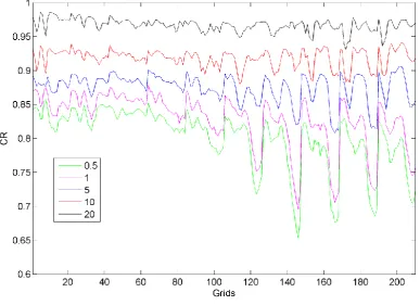
Figure 3.14: Correspondence ratio (CR) for various threshold values for all grids. ... 41
Figure 3.15: Correspondence ratio (CR) for 0.5 mm threshold values for all grids. ... 42
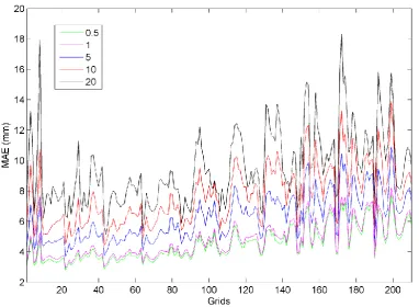
Figure 3.16: Mean absolute error (MAE) for various threshold values for all grids. ... 42
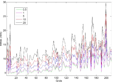
Figure 3.17: Root mean square error (RMSE) for various threshold values for all grids. ... 43
Figure 3.18: Mean absolute error (MAE) for 0.5 mm threshold values for all grids. ... 43
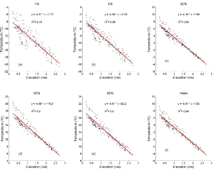
Figure 3.19: Linear regression between elevation and Tn for 5 quantiles and mean value for all grids from 1979-2010. ... 44
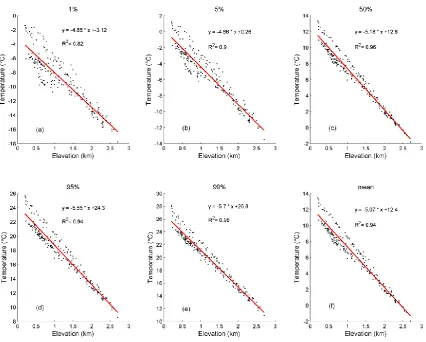
Figure 3.20: Linear regression between elevation and Tg for 5 quantiles and mean value for all grids from 1979-2010. ... 45
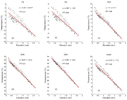
Figure 3.21: Linear regression between elevation and Tx for 5 quantiles and mean value for all grids from 1979-2010. ... 46
Figure 3.22: Boxplots of monthly lapse rates for Tn, Tg, and Tx from 1979-2010.. ... 47
Figure 3.23: Linear regression between elevation and annual precipitation. ... 48
Figure 4.1: Location of the twelve meteorological stations and ERA-Interim grids.. ... 54
Figure 4.2: Schematic illustration of measured lapse rate and ERA-Interim derived lapse rates for Group 1.. ... 56
Figure 4.3: The scatter plots show the comparison of 3-hourly ERA-Interim 2 m temperature and meteorological stations for Group 1. ... 58
Figure 4.4. Boxplots of monthly lapse rates for 4 Groups. ... 60
Figure 4.5: The scatter plots show the comparison of measured and modeled 3-hourly temperatures for Group 1.. ... 65
Figure 4.6: The scatter plots show the comparison of measured and modeled daily temperatures for Group 1.. ... 66
Figure 4.7: Downscaling ERA-Interim temperature at 90 m grid.. ... 67
XIII
Figure 5.2: Estimation picture for Lasso theory. ... 82
Figure 5.3: Percentage of annual precipitation bias between ERA-Interim and MeteoSwiss stations in the period 1983-2010.. ... 85
Figure 5.4: Percentage of annual precipitation bias between observations and four
downscaled, as well as the original ERA-Interim data from 1999-2010. ... 87
Figure 5.5: Taylor diagram of observations with downscaled daily precipitation for 4
downscaling methods as well as the original ERA-Interim data from 1999-2010. ... 96
Figure 6.1: Location of flux sites and ERA-Interim points. ... 100
Figure 6.2: The scatter plots show a comparison of flux sites and ERA-Interim 3-hourly temperatures for IT-LMa from 2002-2006. ... 104
Figure 6.3: Correlation of MAEs and elevation differences for 3-hourly temperature.. ... 104
Figure 6.4: Plot of 3-hourly precipitation at ES-ES1 and ES-ES2 site as well as ERA-Interim in 2006. ... 109
Figure 6.5: Correlation of MAEs and elevation differences for 3-hourly precipitation.. ... 110
Figure 6.6: Plot of daily precipitation at IT-BCi and FR-Gri sites as well as ERA-Interim in 2006... 111
Figure 7.1: Technical flow of map production ... 115
Figure 7.2: The scatter plots show the comparison of daily ERA-Interim 2 m temperatures and measurements for Berlin. ... 119
Figure 7.3: The scatter plots show the comparison of daily ERA-Interim 2 m temperatures and measurements for Istanbul. ... 119
Figure 7.4: Global temperature distribution for 0.1 % and 99.9% quantiles. ... 119
Figure 7.5: Southern European temperature distribution for 0.1 % and 99.9% quantiles. ... 119
Figure A.1: Taylor diagrams for all 50 MeteoSwiss stations. ... 157
Figure A.2: Global temperature distribution for eight quantiles. ... 157
XV
List of Tables
Table 1.1: Literature review of dynamical downscaling studies. ... 5
Table 1.2: A summary of the strengths and weaknesses of the main statistical downscaling methods. ... 6
Table 1.3: Main available reanalysis productions... 8
Table 3.1: Fixed monthly lapse rates. ... 29
Table 4.1: Test sites information. ... 54
Table 4.2: Applied lapse rate and reference temperature of four correction methods for twelve test stations. ... 57
Table 4.3: Comparison of ERA-Interim 2m temperature with 3-hourly and daily data of twelve meteorological stations.. ... 59
Table 4.4: Comparison of measurements with downscaled 3-hourly and daily data for 4 methods. ... 62
Table 4.5: Comparison of measurements with downscaled 3-hourly and daily data for 4 groups.. ... 63
Table 5.1: Literature review of precipitation downscaling methods... 72
Table 5.2: Used predictors from ERA-Interim dataset ... 75
Table 5.3: Test sites information.. ... 76
Table 5.4: Comparison of ERA-Interim daily precipitation with observations at 50 meteorological stations from 1983-2010.. ... 83
Table 5.5: Comparison of observations with downscaled daily precipitation for 4 downscaling methods as well as original ERA-Interim data in the validation period 1999-2010. ... 87
XVI
Table 5.7: Selected variables in Stepwise and Lasso model.. ... 91
Table 6.1: Flux tower site information. ... 101
Table 6.2. Applied lapse rate and reference temperature for ten flux sites. ... 102
Table 6.3: Comparison of ERA-Interim 2 m temperature with 3-hourly data of 48 flux sites.. ... 103
Table 6.4: Comparison of measurements with the original ERA-Interim 3-hourly 2 m
temperatures and downscaled results for 10 flux sites.. ... 106
Table 6.5: Comparison of ERA-Interim precipitation with 3-hourly and daily data of 48 flux sites.. ... 107
Table 7.1: Duration for each quantile ... 114
Table 7.2: City information. ... 118
Table 7.3: Comparison of ERA-Interim 2 m temperature with daily data of nine
meteorological stations.. ... 120
Table A.1: N128 Reduced Gaussian grid ... 139
XVII
List of Symbols and Abbreviations
Symbols
p
a The fraction of precipitation in the grid cell
lA , A
a Rate of change of cloud water/ice and cloud area due to transport throughthe boundaries of the grid volume.
pdry
c Specific heat at constant pressure of dry air (J g-1 °C-1)
pvap
c Specific heat at constant pressure of water vapor (J g-1 °C-1)
p
c Specific heat at constant pressure of moist air (J g-1 °C-1)
CP Convective Precipitation (mm)
cld
E Rate of evaporation of cloud water/ice
FG10 10 meter wind gust (m s-1)
prec
G Rate of generation of precipitation from cloud water/ice
g The acceleration of gravity (m s-2 )
H850, H700, H500 Geopotential height at 850 hpa, 700 hpa and 500 hpa (m)
lH The ratio of cloudy in the grid area
LSP Large scale precipitation (mm)
MSLP Mean sea-level pressure (hPa)
cld
P precipitation in cloudy situation (mm)
clr
P precipitation in clear sky (mm)
PERA ERA-Interim precipitation (mm)
POBS Observed precipitation (mm)
l
q Specific humidity at lowest model level (kg kg-1)
surf
q Specific humidity at surface (kg kg-1)
RH850, RH 700, RH 500 Relative humidity at 850 hpa, 700 hpa and 500 hpa (%)
rr Daily total precipitation (mm)
SH850, SH 700, SH 500 Specific humidity at 850 hpa, 700 hpa and 500 hpa (kg kg-1)
conv
S , aconv
XVIII
strat
S , astrat
Rate of formation of cloud water/ice and cloud area by stratiform condensation processes
l
s Dry static energy at lowest model level (kJ kg-1)
surf
s Dry static energy at surface (kJ kg-1)
T850, T700, T500 Temperature at 850 hpa, 700 hpa and 500 hpa (°C)
T3h 3-hourly air temperature (°C)
Ta Near surface air temperature (°C)
Td Daily air temperature (°C)
TCW Total column water (mm)
TERA_2m ERA-Interim 2m temperature (°C)
TERA_850 ERA-Interim temperature at the 850hPa pressure level (°C)
Tg Daily average temperature (°C)
Tn Daily minimum temperature (°C)
Tref Reference temperature (°C)
Tx Daily maximum temperature (°C)
U10 10 meter U wind component (m s-1)
V10 10 meter V wind component (m s-1)
WS10 Wind speed at 10m (m s-1)
Г Lapse rate (°C km-1)
Г700_850 Lapse rate between 700hPa and 850hPa pressure level (°C km-1)
Г700_925 Lapse rate between 700hPa and 925hPa pressure level (°C km-1)
Г850_925 Lapse rate between 850hPa and 925hPa pressure level (°C km-1)
ГE-OBS Lapse rate from E-OBS dataset (°C km-1)
ГKunkel Lapse rate from literature (°C km-1)
h
Elevation difference (m)
*
T Surface temperature (°C)
Constant lapse rate -6.5 °C km-1
l
T Temperature at the lowest model level (°C)
surf
p Surface pressure (hPa)
l
p Lowest model level pressure (hPa)
x
T 290.5 K
y
XIX
2
z Height of screen level observation (2 m)
l
z Height of the lowest model level (m)
H
z0 Roughness length for heat (m)
HWMO
z0 Roughness length for heat at SYNOP station (m)
Q
z0 Roughness length for moisture (m)
QWMO
z0 Roughness length for moisture at SYNOP station (m)
surf
Surface geopotential (m2 s-2)
evap a
Rate of decrease of cloud area due to evaporation
M
The exchange coefficient for momentum at surface
Abbreviations
20CR NOAA-CIRES 20th Century Reanalysis V2
4D-Var Four-Dimensional Variational Assimilation
ASR Arctic System Reanalysis
BPRC-PMG Byrd Polar Research Center, Polar Meteorology Group
cdf Cumulative distribution function
CFSR NCEP Climate Forecast System Reanalysis
CHRM An adaptation of HRM, Swiss Federal Institute of Technology (ETH)
COR Weighted pattern correlation
CR Corresponding Ratio
CRIEPI The Central Research Institute of Electric Power Industry
CRU Climate Research Unit
DD Dynamical Downscaling
DKRZ Deutsches Klimarechenzentrum
DWD German Weather Service
ECA&D European Climate Assessment and Dataset
ecdf Empirical Cumulative distribution function
ECMWF European Centre for Medium-Range Weather Forecasts
ENSEMBLES Project from European Commission's 6th Framework Program
E-OBS E-OBS gridded dataset from ECA&D
ERA-15 ECMWF Re-analysis 15 Project
ERA-40 ECMWF Re-analysis 40 Project
XX
GCM Global Climate Model or Global Circulation Model
GCOS The Global Climate Observation System
GHCND Global Historical Climatology Network
GISS Goddard Institute for Space Studies at NASA
GKSS Gesellschaft für Kommunikation, Schutz und Sicherheit
GLADS Global Land Data Assimilation System
GMAO Global Modeling and Assimilation Office
GPCC Global Precipitation Climatology Centre
GSFC Goddard Space Flight Center
GTS Global Telecommunication System
HadGHCND Gridded daily temperature dataset provided by Hadley centre.
HadRM3 Third generation RCM developed by the Hadley Centre
HIRHAM Regional Atmospheric Climate model by Danish Meteorological Institute
ICTP Abdus Salam International Centre for Theoretical Physics
IPCC Intergovernmental Panel on Climate Change
JMA The Japan Meteorological Agency
KNMI Royal Netherlands Meteorological Institute
Lasso Least absolute shrinkage and selection operator
LMDz4 Laboratoire de Meteorologie Dynamique zoom version 4
LOCI Local Scaling
LWD Bavarian Avalanche Warning Service
MAE Mean absolute error
MAP Mesoscale Alpine Program
MERRA NASA Modern Era Reanalysis for Research and Applications
MM5 The fifth-Generation Penn State/NCAR Mesoscale Model
MOS Model Output Statistic
MPIfM Max Planck Institute for Meteorology
NASA The National Aeronautics and Space Administration
NCAR The National Center for Atmospheric Research
NCEP The National Centers for Environmental Prediction
NSE Nash-Sutcliffe efficiency coefficient
OLS Ordinary least squares regression
OMR Observation Minus Reanalysis
XXI
PP Prefect Prognosis
PWC Physics of Weather and Climate Group
QM Quantile-Mapping
RCA1 Rossby Centre regional Atmospheric model version I
RCM Regional Climate Model
RegCM3 3-dimensional, sigma-coordinate, primitive equation regional climate model
REMO Regional climate model developed by MPIfM, DKRZ, DWD and GKSS
RMSD Normalized root-mean-square difference
RMSE Root mean square error
RSS Root of Sum of Squares
SD Statistical Downscaling
SF Scaling factor for LOCI
STD Standard deviation
SYNOP Surface synoptic observations
UKMO U.K. Meteorological Office
WCRP The World Climate Research Programme
1
Chapter 1
Introduction
1.1
Background and Motivation
1.1.1
Climate Change and Global Climate Models
Climate change is one of the most important long-term issues which the global community has to face over coming decades. Negative effects of climate change on nature and the human environment, such as temperature increasing and rising sea level have been observed (IPCC, 2007a; IPCC, 2007c). Therefore, accurate investigations and assessments of the impacts of climate change on natural and human systems are highly desired by decision makers and stakeholders (IPCC, 2007b).
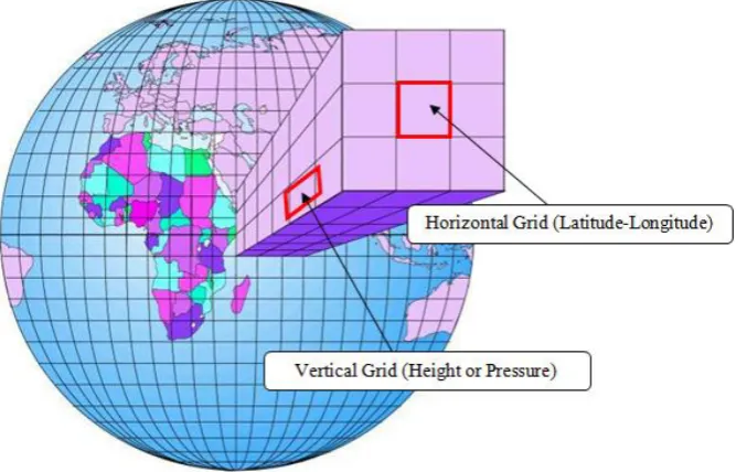
Global Climate Models (or general circulation models, GCMs), the primary tool for weather forecasting, climate understanding, and projecting climate change for the future have been widely applied in the past decades (Gregory et al., 2001; Maraun et al., 2010; Schmidli et al., 2007; Snell et al., 2000; Wilby and Wigley, 2000; Xu, 1999). GCMs attempt to represent the past, present or future climate by simulating the general circulation of the atmosphere, and the oceans, as well as their interaction with powerful computer systems (IPCC, 2007c) (Figure 1.1). GCMs normally run on a 3-dimensional grid with a horizontal resolution of 250-600 km, 10 to 20 vertical layers in the atmosphere and approximately 30 layers in the oceans (e.g. Flato et al., 2000) (Figure 1.2).
2
resolution of 10-50 km, they still do not satisfy the requirements of hydrological and climatic impact models, which typically run on the scale of 0.1-1 km (Ahrens, 2003; Charles et al., 2004; Maraun et al., 2010; Mauser and Bach, 2009; Xu, 1999). Also, RCMs would require very expensive and bring complex computer calculations, making this approach unavailable for many potential users.
Figure 1.1: Schematic of physical processes in Global Climate Models (IPCC, 2007c).
3
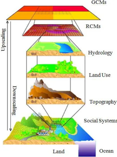
Motivated by the requirements for finer spatial resolution in impact modeling, the scientific community has paid much attention to resolving the scale discrepancy between coarse model data and finer local requirements (Bardossy and Plate, 1992; Charlton et al., 2006; Guan et al., 2009; Hertig and Jacobeit, 2008; Spak et al., 2007). Downscaling procedures – the disaggregation of larger scale mean values to sub-grid smaller scale values – can be used to overcome the deficits of the coarse scale models and to generate meaningful information for areas without meteorological measurements (Maraun et al., 2010; Wilby and Wigley, 1997; Xu, 1999; Zorita and von Storch, 1999). Figure 1.3 schematically illustrates the theoretic scaling processes. Dynamic atmosphere and ocean processes, as well as hydrology, land use, topography and social systems, are considered within the scaling framework.
Figure 1.3: Schematic for a theoretic downscaling and upscaling framework, modified from Viner and Hulme (1997).
Downscaling techniques are classified into two main categories: dynamical downscaling (DD) and statistical downscaling (SD). In the past two decades, DD (e.g. Almazroui, 2012; Haensler et al., 2011) and SD (e.g. Hofer et al., 2010; Huth et al., 2008) have been widely implemented; however, an universal method for various variables and complex terrains is still lacking.
4
atmosphere and land surface characteristics (Decker et al., 2012; Simmons et al., 2010). However, they are still too coarse for use in the finer spatial resolution of climate and hydrology models (Ahrens, 2003).
In summary, accurate downscaling GCMs and reanalysis data in complex terrain is still a major challenge for alpine areas. To meet this challenge, this dissertation attempts to i) evaluate and validate a newly generated reanalysis dataset, the ERA-Interim produced by European Centre for Medium-Range Weather Forecasts (ECMWF), ii) develop a robust temperature downscaling approach which is independent of observations in mountainous areas, iii) introduce a precipitation downscaling method based on machine learning in complex terrain, iv) validate ERA-Interim in various regions, including large urban area and various vegetation covers, and v) illustrate an example of ERA-Interim application in a socio-economic context.
1.1.2
Downscaling Methods Overview
1.1.2.1 Dynamical Downscaling
Dynamical Downscaling (DD, i.e. RCMs) is one downscaling method that is driven by boundary conditions derived from a GCM at high-resolution for a limited area (Wilby and Wigley, 1997). Compared with GCMs, DD uses two approaches to achieve a better representation of orographic effects, land-sea contrast, and land surface characteristics, with the help of finer spatial resolution and reduced model time step (Giorgi, 2008; Rummukainen, 2010). One approach is straightforward and uses a high-resolution atmospheric global model (Christensen et al., 2007); the second approach uses a coarse global model with dense variable-resolution grids in limited-areas (Lal et al., 2008).
5
Thirdly, a quite important drawback of RCMs is their high computational demand (Wilby et al., 2004; Wilby and Wigley, 1997). Although RCMs yield better results by using finer temporal-spatial resolution, the computation requirements rise accordingly. Expensive computation adversely limits the number of grids, spatial resolution, and length of time period under investigation (Maraun et al., 2010; Rummukainen, 2010). At present, many RCMs are available that have been developed by various research institutes over the world. Table 1.1 shows a small selection of previous studies using RCMs.
Table 1.1: Literature review of dynamical downscaling studies.
RCMs Predictand Boundary
forcing Vertical/horizontal resolution Region Reference
REMO 2 m
temperature Seasonal precipitation
ERA-40 20-level/18 and 50
km South African (Haensler et al., 2011)
HadRM3 and
CHRM Seasonal heavy
precipitation
HadAM3
HRM 19-level/50 and 20-level/55 km United Kingdom (Haylock et al., 2006)
RCA1 Monthly
Precipitation HadCM2 ECHAM4 19-level/44 km Sweden (Hellstrom et al., 2001) ECHAM4/
ECHAM5
Annual Rainfall
NCEP Reanalysis
19-level/T42 and 23-level/T63
Southern Morocco
(Huebener and
Kerschgens, 2007) CHRM, HadRM3
and HIRHAM Daily precipitation HRM, HadAM3 and
HIRHAM4
20-level/0.5°, level/0.44° and 19-level/0.44°
European
Alps (Schmidli et al., 2007)
MM5 Monthly
Surface temperature
GISS-GCM 20-level /36 km North
America (Spak et al., 2007)
LMDz4 Summer
rainfall
ERA-40 19-level/stretched
grid, 120 points in longitude and 91 points in latitude
Eastern China
(Zou et al., 2010)
UKMO Model Monthly
temperature precipitation
GCM 19-level/0.44° and
19-level/2.5°×3.75° Europe (Murphy, 1999)
1.1.2.2 Statistical Downscaling
6
the local variables from large-scale outputs (Wilby and Wigley, 1997). The main assumptions of SD methods include: predictors from large-scale data should be skillfully and adequately reproduced; the relationships between predictands and predictors remain valid for periods outside the fitting period, especially for future climate scenarios (Harpham and Wilby, 2005; Wilby et al., 2002; Wilby and Wigley, 1997). Compared to DD, SD methods have lower computational demands and they provide site-specific information in an easier way (Wilby et al., 2002; Wilby et al., 2004; Wilby and Wigley, 1997; Huth, 2004).
Table 1.2: A summary of the strengths and weaknesses of the main statistical downscaling methods, modified from Wilby et al. (2004).
Methods Strengths Weaknesses Examples
Weather typing (e.g. analogue method, hybrid approaches, fuzzy classification, self organizing maps, Monte Carlo methods)
1. Yields physically interpretable linkages to surface climate 2. Versatile (e.g. can
be applied to surface climate, air quality,
flooding, erosion, etc.)
3. Compositing for
analysis of extreme events
1. Requires
additional task of weather
classification 2. Circulation-based
schemes can be insensitive to future climate forcing
3. May not capture
intra-type variations in surface climate
(Alexander et al., 2009; Bardossy et al., 2005; Vrac et al., 2007; Yin et al., 2011;)
Weather generators (e.g. Markov chains, stochastic models, spell length methods)
1. Production of
large ensembles for uncertainty analysis or long simulations for extremes 2. Spatial interpolation of model parameters using landscape
3. Can generate
sub-daily information 1. Arbitrary adjustment of parameters for future climate 2. Unanticipated effects to secondary variables of changing precipitation parameters
(Charles et al., 2004; Greene et al., 2011; Mehrotra and Sharma, 2005) Regression methods (e.g. linear/non-linear regression, neural networks, canonical correlation analysis, kriging) 1. Relatively straightforward to apply
2. Employs full
range of available predictor variables 3. “Off-the-shelf” solutions and software available 1. Poor representation of observed variance
2. May assume
linearity and/or normality of data
3. Poor
representation of extreme events
7
SD methods are classified according to several perspectives. Wilby and Wigley (1997) and Wilby et al. (2004) grouped SD methods into three categories: weather classification schemes, regression models, and weather generators. An alternative classification was presented by Rummukainen (1997) and based on the nature of predictors, namely, prefect prognosis (PP) and model output statistics (MOS). Wilby et al. (2004) have summarized the advantages and drawbacks of three SD methods (Table 1.2).
Regression methods are widely used because they are simple and easy to implement. Multiple regression (Murphy, 1999), canonical correlation analysis (Vonstorch et al., 1993), and artificial neural networks (Cannon, 2007; Crane and Hewitson, 1998) are most frequently applied. Support vector machines based on machine learning algorithms, are becoming popular (Anandhi et al., 2009; Chen et al., 2010; Kumar et al., 2008; Kumar et al., 2009). Based on their strengths, this study used regression methods for temperature and precipitation downscaling. To avoid repetition, the applied temperature and precipitation downscaling methods are described in Chapters 4 and 5, respectively.
1.1.3
Reanalysis Data – State of the Art
Reanalysis data is produced by a data assimilation project that incorporates observations into a computer model of the atmospheric, land surface, and ocean real system. Data assimilation is implemented by analysis cycles. In each analysis cycle, the current (or past) observations are combined with the results from a forecast model (e.g. numerical weather prediction model). The uncertainty and bias between observations and forecasts are balanced and optimized in this step, and then the advanced model yields new forecasts that are brought into next analysis cycle (Figure 1.4).
Figure 1.4: General view of the reanalysis process.
Reanalysis
Obser-vations
Fore-casts Opti-
8
At present, reanalysis products are provided by four major centers: the National Centers for Environmental Prediction/National Center for Atmospheric Research (NCEP/NCAR), the European Centre for Medium-Range Weather Forecasts (ECMWF), the National Aeronautics and Space Administration (NASA) Goddard Space Flight Center (GSFC), and the Japan Meteorological Agency (JMA) & the Central Research Institute of Electric Power Industry (CRIEPI). Table 1.3 summarizes the main available reanalysis productions. More details including model descriptions can be found in the relevant references.
The key strengths that reanalysis products contain are: i) data is multivariate, spatially and temporally completed and gridded; ii) observations are assimilated; iii) data is physically and dynamically modeled. In the past two decades, reanalysis products have been increasingly applied in climate impact studies. Typically, they are adopted to provide boundary conditions for regional climate models. Although reanalysis products generally estimate the closest state of the real atmosphere and of land surface characteristics (Decker et al., 2012; Simmons et al., 2010), there are some uncertainties in the reanalysis data, such as observation changes and model misrepresentation. Therefore, the quantification of uncertainty and the evaluation of the quality of reanalysis data is still a great challenge (Bosilovich et al., 2008; Trenberth et al., 2008).
Table 1.3: Main available reanalysis products.
Production Time Period Producer Reference
NCEP/DOE Reanalysis II
1979-present NCEP/NCAR (Kanamitsu et al., 2002)
NCEP/NCAR Reanalysis I
1948-present NCEP/NCAR (Kalnay et al., 1996)
ERA-15 1978-1994 ECMWF (Gibson et al., 1996)
ERA-40 Sep. 1957- Aug.2002 ECMWF (Uppala et al., 2005)
ERA-Interim 1979-present ECMWF (Dee et al., 2011; Simmons
et al., 2006)
CFSR 1979-2011 NASA & GSFC (Saha and Coauthors, 2010)
JRA-25 1979-2004 JMA & CRIEPI (Onogi et al., 2007)
JCDAS 2005-present JMA
ASR 2000-2011 OSU & BPRC-PMG (Bromwich et al., 2009;
Hines and Bromwich, 2008)
MERRA 1979-present NASA (Rienecker et al., 2011)
9
10
Figure 1.5: Schematic of the revised 4D-Var solution algorithm implemented in CY25r4. S
denotes the truncation operator which takes the trajectory fields from high to low resolution, J
the cost function and ▽J the gradient of J.x indicates the atmospheric state vector, i the time
index and k the variable index. xb is the initial input, and xa is the result of the loop. δxi is the
analysis increment, and S-1(δx
i) is the minimum increment of δxi. d is the innovation vector, and y
is the observation vector. H(xi) indicates the observation operator with low-resolution in the
vicinity of xi (ECMWF, 2009a).
6-11
hour 4D-Var analysis. The 3-hour 10 days forecasts are obtained from 6-hour 4D-Var analysis, combined with the separate surface analysis.
Figure 1.6: Schematic of data assimilation cycling with the operational early-delivery configuration (ECMWF, 2009a). Yellow means computation steps, and blue data sets.
1.2
Research Objectives
1.2.1
Outline
12
This thesis is structured into five main chapters. Firstly, the usage of ERA-Interim Reanalysis data is investigated in the mountainous areas in Chapter 3. Then, a robust statistical downscaling approach for temperature is presented in Chapter 4, followed by a new precipitation downscaling method in Chapter 5. Subsequently, the validation of the downscaling method using data from micrometeorology station and an application example related to socio-economic work is illustrated in Chapter 6 and 7, respectively. Finally, Chapter 8 gives an overall discussion and outlook for further research activities. The preceding Chapter 2 describes the data resources. A brief description of the core five chapters are presented in the following.
1.2.2
Evaluation of ERA-Interim Reanalysis Data
Generally, GCMs are the primary data resource for downscaling, especially for RCMs. Reanalysis data, currently used as the surrogate for large-scale observations, has been widely applied in downscaling methods such as ERA-40 and NCEP/NCAR reanalysis data (Maraun et al., 2010; Mooney et al., 2011; Poli et al., 2010). Reanalysis data was designed to estimate the closest state of real atmosphere and land surface characteristics with the assimilation of large numbers of observations, which cover complete global and temporal data series. Although reanalysis products are improving, previous studies showed that these products contain errors, due to a variety of reasons, e.g. observation errors and interpolation errors. Therefore, it is of major importance to evaluate reanalysis data against observations before applying them to climate and hydrological models (Berg et al., 2003; Decker et al., 2012; Trenberth and Guillemot, 1998). In Chapter 3, E-OBS, a new observed gridded dataset that interpolated a high density of observations over Europe with finer spatial resolution (0.25°×0.25°) is employed to compare with ERA-Interim 2 m temperature and daily total precipitation data. The bias, as well as the elevation dependence of temperature and precipitation is analyzed.
1.2.3
Temperature Downscaling
A novel method that uses ERA-Interim internal lapse rates for near-surface temperature downscaling in high mountain regions is developed in Chapter 4. This study distinguishes itself from the previous research by i) rejecting the use of the fixed lapse rate (e.g. -6.5 °C km-1) and
13
1.2.4
Precipitation Downscaling
Precipitation downscaling is much more difficult than temperature due to its higher spatial and temporal variability, especially in complex terrains (Barry, 2008; Guan et al., 2009). Although many downscaling methods have been tested, a universal best method does not exist. In Chapter 5, a new and powerful machine learning technique, “Lasso” (Least absolute shrinkage and selection operator), which has the advantage of dealing with large numbers of variables, is explored for downscaling daily total precipitation at 50 meteorological stations in the central Alps. In order to evaluate the performance of the Lasso algorithm, benchmark methods, such as local scaling (LOCI) and quantile-mapping (QM), which are the most frequently used methods for climate impact studies, are applied for model comparison. Additionally, stepwise regression, which uses the same variables, is applied to evaluate the ability of Lasso to deal with the selection of variables.
1.2.5
Validation of ERA-Interim for FLUXNET Data
In Chapter 6, 48 FLUXNET tower sites located in the expanses of land with varying topography and vegetation covers and climate regimes over Europe are applied to validate ERA-Interim data and temperature downscaling methods. FLUXNET is a global network that covers a collection of micrometeorological flux observation sites, measuring the exchanges of carbon dioxide, water vapor, and energy between the biosphere and atmosphere, using eddy covariance methods, but also standard climate data including temperature, relative humidity, precipitation, and radiation components (Baldocchi et al., 2001; Gu and Baldocchi, 2002). Besides temperature, 3-hourly ERA-Interim precipitation data is also validated by FLUXNET data.
1.2.6
ERA-Interim Application - A Case Study
ERA-14
15
Chapter 2
Datasets
2.1
Overview
Throughout this thesis, data from six sources are applied: individual meteorological measurements provided by the German Weather Service (DWD), the Bavarian Avalanche Warning Service (LWD), the European Climate Assessment & Dataset (ECA&D), and the Swiss Federal Office of Meteorology and Climatology (MeteoSwiss); individual micrometeorological measurements provided by FLUXNET; gridded observations (E-OBS) provided by ECA&D, and the Global Precipitation Climatology Centre (GPCC) gridded data provided by DWD; reanalysis data (ERA-Interim) developed by the European Centre for Medium-Range Weather Forecasts (ECMWF). In this chapter, each dataset is briefly introduced and data processing methods are specifically explained in the corresponding chapters.
2.2
DWD and LWD Data
In this study, the observations from two meteorological stations (Zugspitze and Garmisch) operated by the German Weather Service (DWD), as well as one station (Zugspitzplatt) operated by the Bavarian Avalanche Warning Service (LWD) are used for downscaling tests. All three test sites are located in the southern part of Germany, at the Austrian border. The Garmisch site is located at the bottom of a valley (Garmisch-Partenkirchen 719m a.s.l.); the Zugspitze site is close the crest of the Zugspitze mountain (2964m a.s.l.) and the Zugspitzplatt site (2250m a.s.l.) is located on the side of the mountain (Figure 2.1). The DWD provides hourly data, while the LWD operates at 10-minute resolution. The data was aggregated to 3-hourly (T3h) and daily (Td)
16
Figure 2.1: Locations of the DWD and LWD observation sites.
2.2
MeteoSwiss Data
17
2.3
ECA&D Data
The ECA&D (European Climate Assessment & Dataset) project focused on the changes in weather and climate extremes, as well as on the daily dataset needed to monitor and analyze these extremes. This project was initiated by the European Climate Support Network (ECSN) and supported by the Network of European Meteorological Services (EUMETNET). Currently, ECA&D provides a dataset containing 36959 series of observations for 12 elements at 7847 meteorological stations throughout Europe and the Mediterranean from 61 participants in 62 countries (ECA&D, 2013, Klein Tank et al., 2002). The 12 elements include maximum, minimum, mean temperature, sunshine, snow depth, precipitation amount, humidity, wind gusts, wind speed, wind direction and cloud cover. Nine large city sites used for validation of ERA-Interim are listed in Chapter 7. Detailed site information is given in Chapter 7.
2.4
FLUXNET Data
FLUXNET is a global collection of micrometeorological flux observation sites, measuring the exchanges of carbon dioxide, water vapor, and energy between the biosphere and atmosphere, using eddy covariance methods, but also standard climate data including temperature and precipitation (Baldocchi et al., 2001; Gu and Baldocchi, 2002). The FLUXNET database is maintained by the Oak Ridge National Laboratory Distributed Active Archive Center (ORNL DAAC).
18
At present, more than 500 tower sites across five continents are operating on a long-term basis covering a large variety of climates and biomes (Figure 2.2). The LaThuile dataset is one of the FLUXNET synthesis data products, and currently includes data from approximately 250 sites, which is available under a “free fair-use” policy (Fluxdata, 2013). From this dataset, 48 sites located in Europe and having a continuous record of at least 2 years have been chosen for ERA-Interim validation. For more details see Chapter 6.
2.5
E-OBS Data
The European daily high-resolution gridded dataset of surface temperature (mean, minimum and maximum) and precipitation (E-OBS) was developed as part of the European Union Framework 6 ENSEMBLES project, with the objective of validating RCM models for climate change studies (Haylock et al., 2008). The E-OBS dataset was produced for representing the best estimates of grid box averages. Gridded 0.25° and 0.5° latitude/longitude data is available, as well as a 0.22° and 0.44° rotated pole grid with the North Pole at 39.25N, 162W (E-OBS, 2013). The available data covers a large area (all of Europe, without oceans) and a long time period (1950-present).
The E-OBS dataset was produced from large number of observations. Daily observations of maximum, mean and minimum temperature, and precipitation were collected since 1950 by the Royal Netherlands Meteorological Institute (KNMI), which also is in charge of European Climate Assessment and Dataset (ECA&D). The number of observation stations increased from 250 at the beginning to currently more than 2300 by incorporation with other datasets, such as GCOS (Global Climate Observing System), GHCND (Global Historical Climatology Network), and MAP (Mesoscale Alpine Program) (Haylock et al., 2008). The quality of the raw observations was controlled and suspicious records were eliminated, based on the criteria of, for example, less than zero and more than 300 mm for precipitation and temperatures higher than 60 °C (Haylock et al., 2008). The measured time at some stations was shifted forwards or backwards by one day between different countries. Maximum and minimum temperatures were calculated from 0000, 0600, 1200 and 1800 UTC. Precipitation was assumed to be measured at 0900 UTC and 0.5 mm threshold was defined for dry/wet day. The values of 0000 and 0600 UTC on the second day were added to 1200 and 1800 UTC values on the first day for the first day record (Haylock et al., 2008).
19
finer than that of HadGHCND (Caesar et al., 2006), which has global gridded daily data projected on a much coarser 2.5° latitude by 3.75° longitude grid as well as that of the MARS-STAT database, which is based on a 50 km grid. The E-OBS covers a long-term period from 1950 to the present, whilst HadGHCND data only spans the period of 1946-2000, and MARS-STAT only started in 1975. Although Alpine precipitation gridded data (Frei and Schar, 1998) was developed at a spatial resolution of 25km, it was only available for the period 1971-1990.
Given its strengths, this study applied the E-OBS dataset to evaluate ERA-Interim data. Daily maximum, mean and minimum temperature, and precipitation on a 0.25°×0.25° spatial resolution from E-OBS version 6.0, which was released in April 2012 and which covers the period from 1950-2011, was retrieved from E-OBS datasets. This evaluation is specifically illustrated in Chapter 3.
2.6
GPCC Data
The GPCC data is a contribution of the German Weather Service (DWD) to the World Climate Research Program (WCRP) and to the Global Climate Observation System (GCOS) (Schneider et al., 2011). GPCC represents long-term monthly land surface precipitation derived from rain-gauges built on the Global Telecommunication System (GTS) and from historic data for global and regional climate monitoring and research (Meyer-Christoffer et al., 2011). GPCC data is available on a regular latitude/longitude grid with a spatial resolution of 0.25°, 0.5°, 1.0°, and 2.5°. In this study, GPCC Climatology Version 2011, based on the 67,200 stations world-wide that have record durations of 10 years or longer for the target reference period January 1951 to December 2000 is applied for the evaluation of the ERA-Interim precipitation product. The data can be downloaded via: ftp://ftp.dwd.de/.
2.7
ERA-Interim Reanalysis Data
20
resolution with 31 vertical hybrid levels (ECMWF, 2013). The extended reanalysis data ERA-40 was generated from September 1957 to August 2002, and has been extensively utilized for atmospheric and oceanic processes. ERA-40 was assimilated at T159 spectral resolution (1.125 ° × 1.125 °) with 60 vertical hybrid levels. The results were projected on a reduced Gaussian grid (N80) with an almost uniform spacing of ~125km, the same as for ERA-15 (Uppala et al., 2005). As the second generation of reanalysis data, ERA-40 is superior to ERA-15, which has been well illustrated by Uppala et al. (2005).
Based on ERA-40, ERA-Interim represents a third generation reanalysis product with an improved atmospheric model and assimilation system. ERA-Interim provides data from 1979 onwards, and continues in real time (Berrisford et al., 2009; Dee et al., 2011). The ERA-Interim project was launched in order to improve key aspects of ERA-40, such as the representation of the hydrological cycle, the quality of the stratospheric circulation, as well as the handling of biases and changes in the observing system (Dee and Uppala, 2009; Dee et al., 2011; Simmons et al., 2006; Uppala et al., 2008). This has been achieved by including many model improvements, such as the use of 4-dimensional variation analysis, a revised humidity analysis, the use of variation bias correction for satellite data, and other improvements in data handling (Berrisford et al., 2009; Dee et al., 2011). Cycle 31r2 of ECMWF’s Integrated Forecast System (IFS) was used for the ERA-Interim product. In this configuration, the model comprises 60 vertical levels, with the top level at 0.1 hPa; it uses the T255 spectral harmonic representation for the basic dynamical fields and a reduced Gaussian grid (N128, Figure 2.3, see section A.1) with an approximately uniform spacing of 79 km (Dee et al., 2011; Uppala et al., 2008). For more detailed model description, see the series report of ECMWF (ECMWF, 2013).
21
targets - temperature and precipitation - are introduced briefly in the next two sections, based on an ECMWF technical series report (ECMWF, 2009b).
Figure 2.3: Reduced Gaussian Grid N128.
2.7.1
2 m Temperature
In the ERA-Interim model (IFS CY31r2), the 2 m temperature is interpolated between the lowest model level (about 10 m above the surface in the 60-level model) and the surface temperature by making use of the profile functions, which are similar for other surface fluxes. The 2 m temperature is derived from Eq. 2.1.
c
q
T
gz
c
T
s
pdry1
p (2.1)with 1
pdry pvap
c c
(2.2)
where,
s
andq
are the dry static energy and specific humidity, respectively. cpdry, cpvap and cpare the specific heats at constant pressure of dry air, water vapor, and moist air, separately, and
is the geopotential. g is the acceleration of gravity.
s
andq
at 2 m level are calculated from Eq.22 L z L z z z z z L z L z z z z z s s s s HWMO M MWMO l M HWMO MWMO l HWMO M MWMO M HWMO MWMO surf l surf 0 0 0 0 0 0 2 0 0 2 2 log log )
( (2.3)
L z L z z z z z L z L z z z z z q q q q QWMO M MWMO l M QWMO MWMO l QWMO M MWMO M QWMO MWMO surf l surf 0 0 0 0 0 0 2 0 0 2 2 log log )
( (2.4)
where, ssurf and qsurf is the dry static energy and specific humidity at the surface, respectively.
Similarly, sland qlare at lowest model level. z2is 2 m, zlis the height of the lowest model level
and z0HWMO and z0QWMO are roughness lengths, which both equal to 0.003 when larger than 0.03,
otherwise z0HWMO equals to z0H and z0QWMO equals to z0Q. L is the Obukhov length. M
represents the exchange coefficient for momentum at the surface. The subscript WMO means WMO reporting practice (ECMWF, 2009b).
2.7.2
Total Precipitation
Total precipitation is comprised of convective precipitation (CP) and large scale precipitation (LSP or stratiform precipitation) from various sources, pure ice clouds, pure water clouds and mixed phases. Because microphysical processes are different in clear and cloudy skies, the precipitation is assimilated in these two parts separately (ECMWF, 2009b). The precipitation (P) is summarized by:
clr cld
P P
P (2.5)
where, Pcldis the precipitation in the cloudy situation, while Pclr is for clear sky. They are calculated separately, based on Eq. 2.6 and 2.7.
dA
l H P APcld 1
(2.6)
H l
dAP A
23
where, H
l represents the ratio of cloudy in the grid area A with the specific humidityl. The fraction of precipitation ap in the grid cell is obtained by:clr p cld p p a a
a (2.8)
dA
l H P HA acld
p
1 (2.9)
H l dA
H PA aclrp
11 (2.10)
Here, only the basic equations for the time change of the grid-box averaged cloud water/ice content are given and the cloud fraction is obtained by:
l Sconv Sbl Sstrat Ecld GprecA t
l
(2.11)
a aconv astrat aevapA t
a
(2.12)
The variables and notations in Eq. 2.11 and 2.12 represent the following processes:
lA , A
a Rate of change of cloud water/ice and cloud area due to transportthrough the boundaries of the grid volume.
conv
S , aconv Rate of formation of cloud water/ice and cloud area by convective
processes
strat
S , astrat Rate of formation of cloud water/ice and cloud area by stratiform
condensation processes
cld
E Rate of evaporation of cloud water/ice
prec
G Rate of generation of precipitation from cloud water/ice
evap a
Rate of decrease of cloud area due to evaporation
25
Chapter 3
Evaluation of ERA-Interim
Reanalysis Data
3.1
Introduction
Reanalysis products are widely applied in climate impact studies. Typically they are adopted to provide boundary conditions for regional climate models. Reanalysis products contain the following key strengths: i) data is multivariate, spatially and temporally completed, and gridded; ii) observation are assimilated; iii) data is physically and dynamically modeled. Generally, reanalysis products estimate the closest state of real atmosphere and land surface characteristics (Decker et al., 2012; Simmons et al., 2010). However, there are some uncertainties related to reanalysis data such as observation errors and model misrepresentation. The quantification of uncertainty in reanalysis data is a serious challenge. At present, reanalysis products are provided by four major centers: NCEP/NCAR Reanalysis from the National Centers for Environmental Prediction/National Center for Atmospheric Research (NCEP/NCAR), ERA-15, ERA-40 and ERA-Interim from the European Centre for Medium-Range Weather Forecasts (ECMWF), the Climate Forecast System Reanalysis (CFSR) from the National Aeronautics and Space Administration (NASA) Goddard Space Flight Center (GSFC), and JAR-15 from the Japan Meteorological Agency (JMA) and the Central Research Institute of Electric Power Industry (CRIEPI) (Table 1.3).
26
(2010), respectively. They found a high temporal correlation (r = 0.997) between CRUTEM3 and ERA-Interim temperature for the period from 1989 to 2001 with respect to Europe. It was shown that the accordance of ERA-Interim and CRUTEM3 is generally good with respect to large-scale patterns and magnitudes (Simmons et al., 2010). For precipitation, ERA-Interim and GPCC have the best agreement for all six continents (Europe, Asia, North America, Africa, Australia and South America). Their diagnosis also indicated that ERA-Interim has sufficient accuracy in continental-scale precipitation for monthly anomalies (Simmons et al., 2010). NCEP/NCAR reanalysis data showed significant bias in moisture fields, especially in the tropics (Trenberth and Guillemot, 1998).
Betts et al. (2009) evaluated the performance of ERA-40 and ERA-Interim temperature, precipitation and shortwave radiation data against observations from three large river basins (Amazon, Mississippi and Mackenzie). The seasonal cycle between two reanalysis data and observation are different for diverse variables and basins. For instance, 40 and Interim have higher 2 m temperature than observations in the Mississippi basin, whereas ERA-Interim increases the precipitation and ERA-40 drifts the annual precipitation over the Amazon (Betts et al., 2009). ERA-Interim has some improvements over ERA-40, which results in a different bias against observations. Belo-Pereira et al. (2011) found ERA-Interim outperformed ERA-40 over the Iberian Peninsula in precipitation. However, the total precipitation was strongly underestimated, due to the mountainous topography.
Decker et al. (2012) evaluated air temperature, wind speed, precipitation, downward shortwave radiation, net surface radiation, and latent and sensible fluxes from GSFC, NCEP, and ECMWF reanalysis datasets, using 33 FLUXNET flux towers. The results showed that ERA-Interim performed best in terms of variability for 6-hourly air temperature, and ERA-40 had the lowest bias in latent flux and precipitation. The variability of 6-hourly precipitation was best assimilated by GLDAS and ERA-Interim datasets (Decker et al., 2012).