Isomorphism classes of Edwards curves over
finite fields
Reza Rezaeian Farashahi
Department of Computing
Macquarie University
Sydney, NSW 2109, Australia
and
Department of Mathematical Sciences
Isfahan University of Technology
P.O. Box 85145 Isfahan, Iran
[email protected]
Dustin Moody
National Institute of Standards and Technology (NIST)
100 Bureau Drive, Gaithersburg, MD, 20899, USA
[email protected]
Hongfeng Wu
College of Sciences
North China University of Technology
Beijing 100144, P.R. China
[email protected]
Abstract
Edwards curves are an alternate model for elliptic curves, which have attracted notice in cryptography. We give exact formulas for the number of Fq-isomorphism classes of Edwards curves and twisted
1
Introduction
Elliptic curves have been an object of much study in mathematics. Recall that an elliptic curve is a smooth projective genus 1 curve, with a given rational point. The traditional model for an elliptic curve has been the Weierstrass equation
Y2+a1XY +a3Y =X3+a2X2+a4X+a6,
where the ai are elements in some field F. While other models for elliptic curves have long been known, in the past few years there has been renewed interest in these alternate models. This attention has primarily come from the cryptographic community.
In 2007, Edwards proposed a new model for elliptic curves [10]. LetFbe a field with characteristic p6= 2. These original Edwards curves, defined over F, are given by the equation
EE,c : X2+Y2 =c2(1 +X2Y2), (1)
withc∈Fandc5 6=c. Edwards curves and its variants over finite fields have attracted great interest in elliptic curve cryptography (see [2, 3, 4, 5, 6]). In particular, Bernstein and Lange [3] have considered the closely related family of Edwards curves
EBL,d : X2+Y2 = 1 +dX2Y2, (2)
where d ∈ F with d 6= 0,1. They also considered the generalization of this family, the so-called twisted Edwards family, [2], given by
ETE,a,d : aX2 +Y2 = 1 +dX2Y2, (3)
where a, d are distinct nonzero elements of F, with d 6= 1. In the same paper, they show that a twisted Edwards curve is birationally equivalent to a Montgomery curve. We recall, [18], that an elliptic curve given by a Montgomery equation is of the form
EM,A,B : BY2 =X3+AX2+X, (4)
where A, B ∈F with A6=±2 and B 6= 0.
curves over Fqup to isomorphism. This has been done for Weierstrass curves [17, 20], and various alternate models of elliptic curves [12, 13, 14, 15, 16]. The number of isomorphism classes of hyperelliptic curves over finite fields has also been of interest [7, 8, 9, 11].
For the Edwards families (1) and (2), Farashahi and Shparlinski gave explicit formulas for the number of distinct elliptic curves (up to isomorphism over the algebraic closure of the ground field). The tool they used was the
j-invariant of an elliptic curve. They remark that it would be interesting to find exact formulas for the number of distinct curves, up to isomorphism over Fq.
The distinction is subtle. Two curves may be isomorphic overFq without being isomorphic overFq. The issue is whether the isomorphism can be given by rational functions defined over Fq orFq\Fq. For cryptography, the finite field Fq is fixed, and calculations are done over Fq – not its algebraic closure Fq. For cryptographic purposes, two elliptic curves which are Fq-isomorphic are essentially the same curve, which is not true if they are only isomorphic over Fq.
In this work, we answer the question of Farashahi and Shparlinski. That is, we find precise formulas for the number of distinct elliptic curves in the Edwards curve families (1) and (2), up to isomorphism over a finite field. We are able to do so by elementary methods. We also answer the same question for the families (3) and (4), i.e., the twisted Edwards and Montgomery curves. This paper is organized as follows. In Section 2 we review some back-ground material about elliptic curves. In Section 3 we find exact formulas for the number ofFq-isomorphism classes of the Edwards curves (1) and (2). We do the same for twisted Edwards (3) and Montgomery curves (4) in section 4. We conclude in Section 5 with some directions for future study.
Throughout the paper, the letter p always denotes a prime number and the letter q always denotes a prime power. Let Fq be a finite field with characteristic greater than 3. For a field F, denote its algebraic closure by F and its multiplicative subgroup by F∗. Let χ denote the quadratic character in Fq. That is, for u ∈ F∗q, χ(u) = 1 if and only if u =w2 for some w ∈Fq. Let Qbe the set of quadratic residues of Fq\ {0,1}, i.e.,
Q={u∈Fq: u6= 0,1, χ(u) = 1}.
2
Elliptic curves
2.1
Background on isomorphisms
We briefly review some material on isomorphisms between elliptic curves. For more details on isomorphisms, or more generally on elliptic curves, see [21, 22]. Two elliptic curves are isomorphic over a field F, if there is an isomor-phism between the two curves which is defined over F. Isomorphisms on Edwards curves have not yet been as well studied as isomorphisms on Weier-strass curves. In order to obtain our results, it will be informative to review what is known about isomorphisms between Weierstrass curves.
It is well known (see e.g. [17]) that two elliptic curves given by Weierstrass equations are isomorphic over F if and only if there is a change of variables between them of the form:
(x, y)→(α2x+r, α3y+α2sx+t),
where α 6= 0, and α, r, s, t ∈ F. In the case, where α, r, s, t ∈ F, the two elliptic curves are called isomorphic over F or twists of each other. We will refer to a change of variables of the above form as an admissible change of variables over F. When the field F is clear from context, we will omit it.
Thej-invariant is a numerical invariant that can be used to tell when two curves are isomorphic over Fq. All of the elliptic curves we will consider in this paper can be represented by the Legendre equation
EL,u : Y2 =X(X−1)(X−u), (5)
for some u∈F∗. The j-invariant of EL
,u is given by
j(EL,u) =
28(u2−u+ 1)3
(u2−u)2 .
Two elliptic curves are Fq-isomorphic if and only if they have the same j -invariant. Farashahi and Shparlinski used this fact to prove their results about the number ofFq-isomorphism classes. Note, however, that two elliptic curves with the same j-invariant need not be isomorphic over Fq.
In the following, we useJE(q), JBL(q),JTE(q),JM(q) and JL(q) to denote
the number of distinct j-invariants of the curves defined over Fq in the fam-ilies (1), (2), (3), (4) and (5) respectively. Moreover, we use IE(q), IBL(q),
2.2
Legendre curves
A Legendre equation is a variant of the Weierstrass equation with just one parameter. Any elliptic curve defined over an algebraically closed field F of characteristic p 6= 2 can be expressed by the Legendre curve EL,u, given by (5), for some u∈F∗.
We consider the curves EL,u given by the Legendre equation (5) over a finite field Fq. We require u 6= 0,1, so that the curve EL,u is nonsingular. The number of distinct isomorphism classes of Legendre curves over Fq has been studied in [12, 13, 16]. To be more precise, for the number JL(q) of
distinct values of the j-invariant of the family (5), we have
JL(q) = b(q+ 5)/6c.
Furthermore, the number IL(q) of Fq-isomorphism classes of the family (5) is
IL(q) =
b(7q+ 29)/24c if q≡1 (mod 12),
b(q+ 2)/3c if q≡3,7 (mod 12),
b(7q+ 13)/24c if q≡5,9 (mod 12),
(q−2)/3 if q≡11 (mod 12).
Now we consider the following subfamily of Legendre curves overFq, and give explicit formulas for its cardinality. We will use the results of this section to count the number of Fq-isomorphism classes of Edwards curves. Recall that Q is the set of quadratic residues ofFq\ {0,1}. Let
LS ={EL,u : u∈ Q}. (6)
We also consider two other subfamilies of Legendre curves over Fq. Let
LS1 ={EL,u: u∈ Q,1−u∈ Q}, (7)
LT ={EL,1−u : u∈ Q}. (8)
As before, we use ILS(q), ILS1(q) and ILT(q) to denote the number of
Fq-isomorphism classes of the families (6), (7) and (8) respectively.
Lemma 2.1. For all elements u, v ∈ Q, we have EL,u ∼=Fq EL,v if and only
if u, v satisfy one of the following:
1. v ∈
2. v ∈
1−u,1−1u,u−u1,u−u1 and χ(−1) = 1.
Proof. See [13, Lemma 2].
Now, we give an exact formula for the number ofFq-isomorphism classes of elliptic curves over Fq of the family (6).
Lemma 2.2. For any prime p≥3, for the number ILS(q)of Fq-isomorphism
classes of the family (6), we have
ILS(q) =
q+ 5 6
, if q ≡1 (mod 4),
q−3
4 , if q ≡3 (mod 4).
Proof. For a fixed value u∈ Q, we let
ILS,u=
v : v ∈ Q, EL,u∼=Fq EL,v .
We note that
ILS(q) =
X
u∈Q
1 #ILS,u
.
We partition Qinto the following sets:
A ∪ B,
where
A =u∈ Q :u6=−1,2,1/2, u2−u+ 16= 0 ,
and B =B1∪ B2 with
B1 ={u∈ Q : u=−1,2,1/2}, B2 =
u∈ Q : u2−u+ 1 = 0 .
We further partitionA into the sets
A1∪ A−1
where
A1 = {u∈ Q : u /∈ B, χ(1−u) = 1},
Now, for all u ∈ Q, we explicitly express the set ILS,u and compute its
cardinality. We note that the sets B1 and B2 are disjoint precisely when
p > 3. If p= 3, we have
B =B1 =B2 ={u∈ Q:u=−1}.
We know that −1 ∈ Q if and only if q ≡ 1 (mod 4). So by Lemma 2.1 we obtain
ILS,−1 =B={−1}, if q ≡9 (mod 12).
We now use the fact that χ(2) = 1 if and only if q ≡ ±1 (mod 8). So, for
p > 3, we have
B1 =
{−1,2,1/2}, if q≡1 (mod 8),
{−1}, if q≡5 (mod 8),
{2,1/2}, if q≡7 (mod 8).
Then, using Lemma 2.1 again, we see that
ILS,u =B1, if u∈ B1.
Next, we assume that u ∈ B2, i.e., u ∈ Fq with u2 −u+ 1 = 0. This happens if χ(−3) = 1 which is equivalent to the case where q ≡1 (mod 6). Then,u= 1+2ζ, whereζ is a square root of −3 inFq. Noticeucan be written as u = −(1−ζ
2 )
2. So, u ∈ Q if and only if q ≡ 1 (mod 4). In other words,
B2 6=∅ if and onlyq ≡1 (mod 12). From Lemma 2.1, we have
ILS,u =B2 ={u,1/u}, if u∈ B2.
Now we consider u∈ A. From Lemma 2.1, we have
ILS,u ={u,1/u}, if u∈ A, q≡3 (mod 4).
Similarly, we also have
ILS,u={u,1/u}, if u∈ A−1, q≡1 (mod 4),
and
ILS,u=
u,1
u,1−u,
1 1−u,
u−1
u , u u−1
Putting this all together, for anyu∈ Q, we have
#ILS,u =
#B1, if u∈ B1,
#B2, if u∈ B2,
2, if u∈ A, and q ≡3 (mod 4),
2, if u∈ A−1, and q≡1 (mod 4),
6, if u∈ A1, and q ≡1 (mod 4).
Now we observe that
ILS(q) =
P
u∈Q
1 #ILS ,u =
P
u∈B
1 #ILS ,u +
P
u∈A
1 #ILS ,u.
We distinguish the following cases for q.
• First, we assume that χ(−1) =−1, i.e., q ≡3 (mod 4). The set B2 is
the empty set. Furthermore, the setB1 is nonempty if and only ifq≡7
(mod 8). In the latter case, we have #B1 = 2 and #A= #Q −#B1 =
(q−3)/2−2. If the set B1 is empty, then #A = #Q= (q−3)/2. We
see that either way we obtain
ILS(q) = (q−3)/4.
• Second, we assume that χ(−1) = 1, i.e., q≡1 (mod 4). If p= 3, then
P
u∈B
1
#ILS ,u = 1. Forp > 3, we write
P
u∈B #IL1S ,u =
P
u∈B1
1 #ILS ,u+
P
u∈B2
1 #ILS ,u =
P
u∈B1
1 #B1+
P
u∈B2
1 #B2.
In this case, the setB1 is nonempty and the set B2 is nonempty if and
only if q≡1 (mod 12).Therefore, we have
X
u∈B
1 #ILS,u
=
2, if q≡1 (mod 12),
1, if q≡5,9. (mod 12). (9)
Next, we write
P
u∈A #IL1S ,u =
P
u∈A1
1 #ILS ,u+
P
u∈A−1
1 #ILS ,u =
P
u∈A1
1 6+
P
u∈A−1
1 2.
So, we have
X
u∈A
1 #ILS,u
= #A1 6 +
#A−1
For j ∈ {−1,1}, let
Sj ={u:u∈ Q, χ(1−u) =j}.
We note that, Aj =Sj \ B. From [13, Lemma 4], for q ≡ 1 (mod 4), we have
#Sj =
(q−5)/4, if j = 1,
(q−1)/4, if j =−1.
Then, by excluding the elements of B from the sets S1, S−1, we
ob-tain the cardinalities of the sets A1, A−1, where q ≡ 1 (mod 24); see
Table 1, where we let q≡r (mod 24).
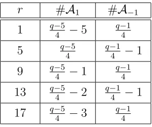
r #A1 #A−1
1 q−45 −5 q−41
5 q−45 q−41 −1
9 q−45 −1 q−41
13 q−45 −2 q−41 −1
17 q−45 −3 q−41
Table 1: Cardinalities of the sets A1,A−1, forq ≡1 (mod 4)
Finally, combining (9), (10) and Table (1), we compute:
ILS(q) =
(q+ 5)/6, if q ≡1 (mod 12),
(q+ 1)/6, if q ≡5 (mod 12),
(q+ 3)/6, if q ≡9 (mod 12),
(q−3)/4, if q ≡3 (mod 4),
which completes the proof of this lemma.
Lemma 2.3. For any primep≥3, for the numberILS1(q)ofFq-isomorphism
classes of the family (7), we have
ILS1(q) =
b(q+ 23)/24c if q ≡1,9,13,17 (mod 24),
(q−5)/24 if q ≡5 (mod 24),
(q−3)/4 if q ≡3 (mod 4).
Proof. Let
Q1 ={u∈ Q : χ(1−u) = 1}.
From [13, Lemma 4], we have #Q1 = (q−3)/4. For a fixed value u ∈ Q1,
we let
ILS1,u =
v : v ∈ Q1, EL,u ∼=Fq EL,v .
We note that
ILS1(q) =
X
u∈Q1
1 #ILS1,u
.
So, we need to compute the cardinality of the set ILS1,u for all u∈ Q1.
Forq≡3 (mod 4), we have χ(−1) =−1. For u∈ Q1, we have
χ(1−1/u) = χ((u−1)/u) = χ(u−1) =χ(−1)χ(1−u) =−χ(1−u).
So, 1/u6∈ Q1. Then, from Lemma 2.1, we have
ILS1,u={u}, if u∈ Q1.
Hence,
ILS1(q) =
X
u∈Q1
1 = #Q1 = (q−3)/4.
From now on, we assume that q ≡ 1 (mod 4). We use the proof of Lemma 2.2 and notice that, for v ∈ Q, we have v ∈ ILS1,u if and only if
v ∈ ILS,u and v ∈ Q1.
Foru∈ Q1, let v ∈ ILS1,u. From Lemma 2.1, we have
v ∈ {u,1/u,1−u,1/(1−u), u/(1−u),1−1/u}.
Since χ(u) =χ(1−u) =χ(−1) = 1, we see that χ(v) =χ(1−1/v) = 1. So,
v ∈ Q1, i.e., for u∈ Q1, we have ILS1,u=ILS,u Then, we write
ILS1(q) =
X
u∈Q1
1 #ILS1,u
= X u∈Q1
1 #ILS,u
= X
u∈B∩Q1
1 #ILS,u
+ X u∈A∩Q1
1 #ILS,u
We have
X
u∈B∩Q1
1 #ILS,u
= X
u∈B1∩Q1
1 #ILS,u
+ X
u∈B2∩Q1
1 #ILS,u
.
From the proof of Lemma 2.2, we see that, for p > 3, B1 ∩ Q1 is nonempty
if and only if q ≡ 1 (mod 8) and B2∩ Q1 is nonempty if and only if q ≡ 1
(mod 12). Furthermore,
X
u∈B
1 #ILS,u
=
2, if q ≡1 (mod 24),
0, if q ≡5. (mod 24).
1, if q ≡9,13,17. (mod 24).
(11)
It is easy to see that A ∩ Q1 =A1. Then, from the proof of Lemma 2.2, we
have
X
u∈A1
1 #ILS,u
= #A1 6 .
Then, using equation (11) and Table (1), we obtain
ILS1(q) =
(q+ 23)/24, if q≡1 (mod 24),
(q−5)/24, if q≡5 (mod 24),
(q+ 15)/24, if q≡9 (mod 24),
(q+ 11)/24, if q≡13 (mod 24),
(q+ 7)/24, if q≡17 (mod 24),
which completes the proof.
The following lemma shows the equality of the values ILT(q) and ILS(q)
for all p≥3.
Lemma 2.4. For any prime p ≥ 3, the number ILT(q) of Fq-isomorphism
classes of the family (6) is given by
ILT(q) =
( b(
q+ 5)/6c, if q ≡1 (mod 4),
(q−3)/4, if q ≡3 (mod 4).
α2X + 1 and Y −→ α3Y, where α2 = −1. So, for q ≡ 1 (mod 4), we
obviously have ILT(q) =ILS(q).
If insteadχ(−1) =−1 then the curveEL,1−u is notFq-isomorphic toEL,u, but rather to the nontrivial quadratic twist of EL,u. So, we have
LT =
Et:E ∈ LS ,
where Et is the nontrivial quadratic twist of the elliptic curve E. Hence, for
q ≡1 (mod 4), we see thatILT(q) =ILS(q).
The result now follow by Lemma 2.2.
3
Edwards curves
The numbers of distinct j-invariants of the families of Edwards curve (1) and (2) have been studied in [14, Theorems 3 and 5]. More precisely, for any prime p ≥ 3, the number JE(q) of distinct values of the j-invariant of the
family (1) is
JE(q) =
b(q+ 23)/24c if q ≡1,9,13,17 (mod 24),
(q−5)/24 if q ≡5 (mod 24),
b(q+ 1)/8c if q ≡3 (mod 4).
Also, the numberJBL(q) of distinct values of thej-invariant of the family (2)
is given by
JBL(q) =
(
b(5q+ 7)/12c if q≡1 (mod 4),
b(3q−1)/8c if q≡3 (mod 4).
In the remainder of this section, we find explicit formulas for the numbers of Fq-isomorphism classes of the Edwards families (1) and (2).
We consider the following family of elliptic curves overFq given by
E4,c: Y2 =X3+ (1−2c)X2+c2X, (12)
for c∈ Fq with c6= 0,1/4. The next lemma shows the equivalence between the above family (12) and the family of Edwards curves (2).
Lemma 3.1. Every Edwards curve EBL,d given by (2) over Fq with d6= 0,1
Proof. We recall from [2] that every elliptic curveE(Fq) with a point of order 4 is birationally equivalent to an Edwards curve EBL,d . It is easy to verify that P = (c, c) is a point of order 4 on the curve E4,c, and so the curve is birationally equivalent to a BL-Edwards curve.
Conversely, via the map ψ :EBL,d →E4,(1−d)/4
ψ(x, y) =c(1 +y) 1−y ,
c(1 +y)
x(1−y)
,
we have that the Edwards curveEBL,dis birationally equivalent to the elliptic curve E4,c, with c= (1−d)/4. The inverse is the map
ψ−1(x, y) =x
y, x−c x+c
.
This proves the lemma.
We now partition the Edwards curves (2) into two subfamilies. Recall that Q is the set of quadratic residues ofFq\ {0,1}. Let
BLS ={EBL,d : d ∈ Q}, (13)
and
BLT ={EBL,d : d6∈ Q}. (14)
As before, we useIBLS(q) andIBLT(q) to denote the numbers ofFq-isomorphism classes of this families (13) and (14).
Note that a point P = (x, y) on the curve E4,c has order 2 if and only if y = 0. There is always at least one rational point (0,0) of order 2, and possibly three points. The next remark shows how the number ofFq-rational points of order 2 relates to IBLT(q) and IBLS(q).
Remark 3.2. From Lemma 3.1, we know that every Edwards curve EBL,d is
birationally equivalent to the elliptic curve E4,c withd= 1−4c. Let δc be the
discriminant of the polynomial X2+ (1−2c)X+c2. We have
δc= (1−2c)2 −4c2 = 1−4c=d.
We see that E4,c(Fq) has a single rational point of order 2 if and only if
χ(δc) = χ(d) =−1. Similarly, E4,c(Fq) has three rational points of order 2if
and only if χ(δc) = χ(d) = 1.
Therefore, for the Edwards curve EBL,d, the group EBL,d(Fq) has a single
point of order 2 if and only if EBL,d ∈ BLT. Also, the group EBL,d(Fq) has
Lemma 3.3. For any prime p≥ 3, the number IBLT(q) of Fq-isomorphism
classes of the family (14) is
IBLT(q) = (q−1)/2.
Proof. By Lemma 3.1 and Remark 3.2, we can represent Edwards curves
EBL,d with d 6∈ Q using elliptic curves of the form E4,c with c= (1−d)/4. There are (q−1)/2 non-squares d inFq.
Suppose two Edwards curve, sayEBL,d1andEBL,d2, are isomorphic overFq.
Then the associated curves E4,c1 and E4,c2, with c1 = (1−d1)/4 and c2 =
(1−d2)/4, must be isomorphic overFq as well. The only admissible change of variables from E4,c1 to E4,c2 has α = 1, and r = s = t = 0 (see §2.1).
Therefore, c1 =c2 and d1 =d2. This shows each distinct non-square d leads
to a different isomorphism class. Hence, we have IBLT(q) = (q−1)/2.
We now turn our attention to the second case, i.e., the curves inBLS.
Lemma 3.4. For any primep≥3, for the numberIBLS(q)ofFq-isomorphism
classes of the family (13), we have
IBLS(q) =
(
b(q+ 5)/6c, if q ≡1 (mod 4),
(q−3)/4, if q ≡3 (mod 4).
Proof. Again, from Lemma 3.1 and Remark 3.2, we can represent an Edwards curve EBL,d with d∈ Qusing the curve E4,c with c= (1−d)/4. We write
X3+ (1−2c)X2+c2X =X(X+s2)(X+t2),
where s= 1+2δ, t= 1−2δ and δ2 =d.
First, we assume that q≡1 (mod 4). We then have −1∈ Q. Let i∈Fq such that i2 = −1. The elliptic curve E
4,c is isomorphic over Fq to the Legendre curve EL,u:Y2 =X(X−1)(X−u) with u= (t/s)2, via the map
(x, y)→(x/(is)2, y/(is)3).
Conversely, the Legendre curve EL,u with u = γ2 for some γ ∈ Fq, is iso-morphic to the elliptic curve E4,(1−d)/4 with d = (11+−γγ)2. Hence, for q ≡ 1
(mod 4), the curve family BLS is isomorphic to the curve family LS given by (6). Then, from Lemma 2.2, we have
IBLS(q) =
(q+ 5)/6, if q≡1 (mod 12),
(q+ 1)/6, if q≡5 (mod 12),
Second, we assume that q ≡ 3 (mod 4). The elliptic curve E4,c is iso-morphic over Fq to the Legendre curve EL,u with u = 1 −(t/s)2, via the map
(x, y)→(x/s2+ 1, y/s3).
Conversely, the Legendre curve EL,u with χ(1−u) = 1, where 1−u=γ2 for some γ ∈ Fq, is isomorphic to the elliptic curve E4,(1−d)/4 with d = (11+−γγ)2.
Therefore, for q ≡ 3 (mod 4), the curve family BLS is isomorphic to the curve family LT given by (8). Then, from Lemma 2.4, we have
IBLS(q) = (q−3)/4, if q ≡3 (mod 4).
This concludes the proof of this lemma.
Combining everything, we obtain the total number of Fq isomorphism classes of Edwards curves.
Theorem 3.5. For any prime p≥3, the number IBL(q) of Fq-isomorphism
classes of the family (2), is given by
IBL(q) =
2q+ 1 3
if q≡1 (mod 4),
3q−5
4 if q≡3 (mod 4).
Proof. We clearly have that
IBL(q) =IBLS(q) +IBLT(q).
From Lemmas 3.4 and 3.3, we obtain
IBL(q) =
(2q+ 1)/3, if q ≡1 (mod 12),
(2q−1)/3, if q ≡5 (mod 12),
2q/3, if q ≡9 (mod 12),
(3q−5)/4, if q ≡3 (mod 4),
which completes the proof.
We note that any Edwards curve EE,c, given by (1), is isomorphic to an Edwards curve EBL,c4 of the form
X2+Y2 = 1 +c4X2Y2
Theorem 3.6. For any primep≥3, for the numberIE(q)ofFq-isomorphism
classes of the family (1), we have
IE(q) =
b(q+ 23)/24c if q≡1,9,13,17 (mod 24),
(q−5)/24 if q≡5 (mod 24),
(q−3)/4 if q≡3 (mod 4).
Proof. We recall that any Edwards curve EE,c, given by (1), is isomorphic to an Edwards curve EBL,c4. From the proof of Lemma 3.4, we can represent
the Edwards curve EBL,c4 using the Legendre curve EL,u, where
u=
1−c2
1+c2 2
if q ≡1 (mod 4),
1−1−c2
1+c2 2
if q ≡3 (mod 4).
We see thatχ(u) = χ(1−u) = 1. So, u,1−u∈ Qand EL,u an elliptic curve in the family LS1 given by (7).
Conversely, the Legendre curve EL,u in LS1 with u= γ
2 and 1−u= λ2
for some γ, λ∈Fq, is isomorphic to the elliptic curve EBL,c4 with
c=
( λ
1+γ if q≡1 (mod 4), γ
1+λ if q≡3 (mod 4).
Therefore, the curve family (1) is isomorphic to the curve familyLS1 given
by (7). Then, we see that IE(q) = ILS1(q) and from Lemma 2.3, we have
ILS1(q) =
(q+ 23)/24, if q≡1 (mod 24),
(q−5)/24, if q≡5 (mod 24),
(q+ 15)/24, if q≡9 (mod 24),
(q+ 11)/24, if q≡13 (mod 24),
(q+ 7)/24, if q≡17 (mod 24),
(q−3)/4, if q≡3 (mod 4).
4
Twisted Edwards curves
We consider the twisted Edwards curvesETE,a,d given by the family (3) over a finite field Fq of characteristic p 6= 2. We note that a, d are in Fq with
It has been shown in [2] that twisted Edwards curves are birationally equivalent to Montgomery curves EM,A,B given by the family (4), where
B(A2−4)6= 0. This can be seen via the mapψ :ETE,a,d →EM,2(a+d)/(a−d),4/(a−d)
ψ(x, y) =1 +y 1−y,
1 +y x(1−y)
. (15)
Furthermore, the Montgomery curve EM,A,B is birationally equivalent to the twisted Edwards curve ETE,a,d where a= (A+ 2)/B and d= (A−2)/B.
We note that, the family (3) is the generalization of the families (1) and (2). Clearly, every Edwards curveEBL,d is a twisted Edwards. Moreover, a twisted Edwards curve ETE,a,d is a twist of the Edwards curve EBL,da. We note that a quadratic twist of EBL,d, which is not isomorphic to EBL,d over Fq, may not be in the family (2). Therefore, the family (3) includes the curves of (2) and the twists of the curves of (2). Moreover, thej-invariant of a curve and the j-invariant of its twist are equal. So, both families have the same number of distinctj-invariants. This establishes the following theorem.
Theorem 4.1. For any prime p ≥3, for the numbers JTE(q) and JM(q) of
distinct Fq-isomorphism classes of the families (3) and (4) respectively, we
have
JTE(q) = JM(q) =
b(5
q+ 7)/12c if q ≡1 (mod 4),
b(3q−1)/8c if q ≡3 (mod 4).
In the remainder of this section, we find explicit formulas for the number of Fq-isomorphism classes of Montgomery curves, which is the same as the number of Fq-isomorphism classes of twisted Edwards curves.
We partition Montgomery curves (4) into the following subfamilies. As usual, let Q be the set of quadratic residues of Fq\ {0,1}.Let
MS =
EM,A,B : A2−4∈ Q , (16)
and
MT =
EM,A,B : A2−46∈ Q . (17)
As before, we useIMS(q) andIMT(q) to denote the numbers ofFq-isomorphism
classes of this families (16) and (17). We now compute the values of IMS(q)
Lemma 4.2. For any primep≥3, for the numberIMS(q)ofFq-isomorphism
classes of the family (16), we have
IMS(q) =
( 2b(q+ 5)/6c, if q≡1 (mod 4),
(q−3)/4, if q≡3 (mod 4).
Proof. We note that the family MS is the set of Montgomery curves overFq with three 2-torsion points. From Remark 3.2, we know the family BLS is the set of Edwards curve EBL,d with three 2-torsion points.
Suppose first q ≡ 1 (mod 4). We recall from [2, Theorem 3.5] that for every Montgomery curve EM,A,B with A4 −4 ∈ Q, exactly one of EM,A,B and its nontrivial quadratic twist EM,A,cB (with χ(c) = −1) is birationally equivalent to an Edwards curve EBL,d. On the other hand, an Edwards curve
EBL,d via the map (15) is birationally equivalent to the Montgomery curve
EM,2(1+d)/(1−d),4/(1−d). This means, there is a 2 : 1 correspondence between
the Montgomery curves of the family MS and the Edwards curves of BLS. Therefore, we have IMS(q) = 2IBLS(q). Thus, from Lemma 3.4, for q ≡ 1
(mod 4), we have
IMS(q) =
(q+ 5)/3, if q≡1 (mod 12),
(q+ 1)/3, if q≡5 (mod 12),
(q+ 3)/3, if q≡9 (mod 12).
When q ≡ 3 (mod 4), every Montgomery curve over Fq is birationally equivalent to an Edwards curve [2]. So, the families (16) and (13) are equiv-alent. So in this case, by Lemma 3.4, we have
IMS(q) =IBLS(q) = (q−3)/4.
Lemma 4.3. For any primep≥3, then the numberIMT(q)ofFq-isomorphism
classes of the family (16) is
IMT(q) =
q−1 2 .
that the family BLT is the set of Edwards curveEBL,d with single 2-torsion point.
For the Montgomery curve EM,A,B in MT, we have A2 −4 6∈ Q. Let
a = (A+ 2)/B and d = (A−2)/B. It follows that exactly one of a and d is a square element of Fq. If a∈ Q, thenEM,A,B has the point (1,
√
a) of order 4. Similarly, if d ∈ Q, then the point (−1,√d) is of order 4. In either case we have that EM,A,B has a point of order 4, and so is birationally equivalent to an Edwards curve in BLT. So, we have
IMT(q) =IBLT(q) = (q−1)/2,
which completes the proof of this lemma.
Theorem 4.4. For any prime p≥ 3, for the numbers ITE(q) and IM(q) of
Fq-isomorphism classes of the families (3) and (4) respectively, we have
ITE(q) = IM(q) =
5q+ 7 6
if q ≡1,9 (mod 12),
5q−1
6 if q ≡5 (mod 12), 3q−5
4 if q ≡3 (mod 4).
Proof. As we have previously stated, every twisted Edwards curve ETE,a,d overFqis birationally equivalent overFqto the Montgomery curveEM, 4
a−d,
2(a+d)
a−d
(see Equation (15)). Conversely, every Montgomery curve EM,A,B is bira-tionally equivalent overFq to the twisted Edwards curveETE,AB+2,AB−2 (see [2, Theorem 3.2]). It follows that the families (3) and (4) have the same number of isomorphism classes over Fq. Therefore,
ITE(q) =IM(q).
For the number IM(q) of Fq-isomorphism classes of the family (4), we clearly have
IM(q) = IMS(q) +IMT(q).
By Lemmas 4.2, and 4.3, we have
IM(q) =
(5q+ 7)/6 if q ≡1 (mod 12),
(5q−1)/6 if q ≡5 (mod 12),
(5q+ 3)/6 if q ≡9 (mod 12),
(3q−5)/4 if q ≡3 (mod 4),
5
Conclusion
In this work we answered a question posed in [14]. That is, we found an exact formula for the number of Fq-isomorphism classes of Edwards curves, original Edwards curves, and twisted Edwards curves.
A natural and related question is to find a formula for the number of distinct isogeny classes for a given family of elliptic curves. Ahmadi and Granger recently were able to do this for Edwards curves [1], and Moody and Wu did the same for Hessian curves [19]. It is an open problem to find similar formulas for most other families of curves. This would include twisted Edwards curves, Jacobi quartics, Jacobi intersections, and Huff curves.
References
[1] O. Ahmadi, R. Granger, On isogeny classes of Edwards curves over finite fields, Preprint, 2011. Available at http://eprint.iacr.org/ 2011/135.pdf. Accessed April 2011.
[2] D. J. Bernstein, P. Birkner, T. Lange, C Peters, Twisted Edwards curves, in: S. Vaudenay (Ed.), Progress in Cryptology – Africacrypt 2008, Lecture Notes in Comput. Sci. 5023, Springer-Verlag, 2008, pp. 389–405.
[3] D. J. Bernstein, T. Lange, Faster addition and doubling on elliptic curves, in: K. Kurosawa (Ed.), Progress in Cryptology – Asiacrypt 2007, Lecture Notes in Comput. Sci. 4833, Springer-Verlag, 2007, pp. 29–50.
[4] D. J. Bernstein, T. Lange, Inverted Edwards coordinates, in: S. Boztas and H.-F. Lu (Eds.), Proceedings of AAECC’2007, Lecture Notes in Comput. Sci. 4851, Springer-Verlag, 2007, pp. 20–27.
[5] D. J. Bernstein, T. Lange, Analysis and optimization of elliptic-curve single-scalar multiplication, in: Finite Fields and Applications - Pro-ceedings of Fq8, Contemp. Math. 461, 2008, pp. 1–20.
[7] Y. Choie, E. Jeong, Isomorphism classes of elliptic and hyperelliptic curves over finite fields, Finite Fields Appl. 10 4 (2004) 583–614.
[8] Y. Choie, D. Yun, Isomorphism classes of hyperelliptic curves of genus 2 over Fq, in: L.M. Batten and J. Seberry (Eds.), Information Security and Privacy, Lecture Notes in Comput. Sci. 2384, Springer-Verlag, 2002, pp. 190–202.
[9] Y. Deng, Isomorphism classes of hyperelliptic curves of genus 3 over finite fields, Finite Fields Appl. 12 2 (2006) 248–282.
[10] H. M. Edwards, A normal form for elliptic curves, Bull. Amer. Math. Soc. 44 (2007) 393–422.
[11] L.H. Encinas, A.J. Menezes and J.M. Masqu´e. Isomorphism classes of genus-2 hyperelliptic curves over finite fields, Appl. Algebra Engrg. Comm. Comput. 13 (2002) 57–65.
[12] R. Farashahi, On the Number of Distinct Legendre, Jacobi, Hessian and Edwards Curves (Extended Abstract), in: Proceedings of the Workshop on Coding theory and Cryptology (WCC 2011), 2011, pp. 37–46. Avail-able at hal.inria.fr/docs/00/60/72/79/PDF/76.pdf.
[13] R. Farashahi, On the Number of Distinct Legendre, Jacobi, Hessian Curves, to appear, 2011. Available at http://arxiv.org/.
[14] R. Farashahi, I. Shparlinski, On the number of distinct elliptic curves in some families, Des. Codes Cryptogr. 54(1) (2010) 83–99.
[15] R. Feng, H. Wu, Elliptic Curves in Huff’s model, Preprint, 2010. Avail-able at http://eprint.iacr.org/2010/390.pdf. Accessed Dec 2010.
[16] R. Feng, and H. Wu, On the isomorphism classes of Legendre elliptic curves over finite fields, Sci China Math 54(9) (2011) 1885–1890. doi: 10.1007/s11425-011-4255-0.
[17] A.J. Menezes, Elliptic Curve Public Key Cryptosystems, Kluwer Aca-demic Publishers, 1993.
[19] D. Moody, and H, Wu, Families of elliptic curves with rational 3-torsion, Preprint, 2011.
[20] R. Schoof, Nonsingular plane cubic curves over finite field, J. Combin. Theory Ser. A 46 (1987) 183–211.
[21] J. H. Silverman, The arithmetic of elliptic curves, Springer-Verlag, Berlin, 1995.