Adaptive Neuro-Fuzzy Inference System for the Computation of the Characteristic Impedance and the Effective Permittivity of the Micro-Coplanar Strip Line

ADAPTIVE NEURO-FUZZY INFERENCE SYSTEM FOR THE COMPUTATION OF THE CHARACTERISTIC IMPEDANCE AND THE EFFECTIVE PERMITTIVITY OF THE MICRO-COPLANAR STRIP LINE

N. Sarikaya

Department of Aircraft Electrical and Electronics Civil Aviation School

Erciyes University Kayseri 38039, Turkey

K. Guney and C. Yildiz

Department of Electrical and Electronics Engineering Faculty of Engineering

Erciyes University Kayseri 38039, Turkey

Abstract—A method based on adaptive neuro-fuzzy inference system (ANFIS) for computing the effective permittivity and the characteristic impedance of the micro-coplanar strip (MCS) line is presented. The ANFIS is a class of adaptive networks which are functionally equivalent to fuzzy inference systems (FISs). A hybrid learning algorithm, which combines the least square method and the backpropagation algorithm, is used to identify the parameters of ANFIS. The effective permittivity and the characteristic impedance results obtained by using ANFIS are in good agreement with the theoretical and experimental results reported elsewhere.

1. INTRODUCTION

MCS line structure has been proposed as a measure to avoid these types of proximity effects. Namely, the structural dimensions of MCS lines are so designed that the characteristic impedance is kept at constant value even when the ground potential is located close to the strip con-ductor. With this structure, the packing density of microwave mono-lithic integrated circuits (MMICs) can be enhanced and shunt element connection between the strip and the upper ground conductor can be easily realized.

MCS lines have been analyzed by many other researchers with the use of different methods, but these methods have some disadvantages. The rectangular boundary division method (RBDM) was used to analyze the MCS line [1], which results in long polynomial formulas for computer aided design (CAD). In another study [2], closed-form design equations for 50 ohm MCS lines were obtained by curve fitting data obtained from RBDM. The lack of any fast closed-form equations for the MCS line is a severe handicap in using the line in microwave circuits. The MCS line has been analyzed and the closed-form design equations are obtained by using conformal mapping method (CMM) [3], but these equations consist of complete elliptical integrals of the first kind which are difficult to calculate. For this reason, the approximate formulas were proposed in calculation of elliptic integrals. Namely, classical techniques used in calculating the characteristic parameters of the MCS line require either tremendous computational efforts in calculating the elliptic integrals and the long polynomial formulas, which can not still make a practical circuit design feasible within a reasonable period of time, or strong background knowledge. Finally, a new method based on artificial neural network (ANN) has been proposed to compute the characteristic parameters of MCS line by Sagirogluand Yildiz [4] as an alternative method to the classical techniques in the literature.

both data and existing expert knowledge about the problem, and good generalization capability features have made neuro-fuzzy systems popular in the last few years [5, 6]. Because of these fascinating features, the ANFIS is used to compute the effective permittivity and the characteristic impedance of the MCS line in this paper. In previous works, we successfully used ANFIS for computing accurately the various parameters of the rectangular, triangular, and circular microstrip antennas, and for tracking multiple targets and estimating the phase inductance of the switched reluctance motors [7–11].

In the following sections, the effective permittivity and the characteristic impedance of MCS line and ANFIS are described briefly and the application of ANFIS to the calculation of the design parameters of the MCS line is explained. The results and conclusion are then presented.

2. THE EFFECTIVE PERMITTIVITY AND THE CHARACTERISTIC IMPEDANCE OF MCS LINE

The MCS line consists of a conductor of width w in parallel with a single infinite coplanar ground located on substrate of thicknesshwith relative permittivityεr, together with a bottom ground plane as shown in Figure 1. The zeroth-order approximation of a quasi TEM structure is assumed. The quasi-TEM analysis of MCS lines is based on the assumption that the air-dielectric interface can be modeled as perfect magnetic walls. Hence, the total capacitance per unit length of MCS line can be computed as the sum of the capacitance of the upper plane (in air) and the lower half plane (in dielectric). The conductor thickness is assumed to be infinitely thin. This approximation is satisfied if the substrate thickness h is larger than the lateral extension of the line (s+w).

s

r h

w

ε

∞

Figure1. Geometry of a MCS line.

characteristic impedance can be written as

εeff = C

Ca (1a)

and

Zo = 1

vphC

(1b) wherevphis the phase velocity of electromagnetic waves,C is the total capacitance per unit length of MCS line, andCa is the capacitance of corresponding line with all dielectrics replaced by air.

Thus, the total capacitance of the MCS line is

C =C1+C2 (2)

where C1 is the capacitance in the upper plane (air) and C2 is the

capacitance in the dielectric.

The capacitance of C1 and C2 are determined by means of the

CMM [3] and can be written as

C1 =ε0

K(k1)

K(k1)

(3a) and

C2=ε0εr

K(k2)

K(k2)

(3b) whereK(ki) andK(ki) are the complete elliptical integrals of the first kind. Thus, the effective permittivity and the characteristic impedance of MCS line can be rewritten, by substituting Eq. (3) in Eq. (1), as

εeff =

1 +εr

K(k2)

K(k2) ·

K(k1)

K(k1)

1 +K _(k

2)

K(k2) ·

K(k1)

K(k1)

(4a)

and

Zo=

120π √_ε

eff

K(k1)

K(k1)

+K(k2)

K(k2)

In Eq. (3) and Eq. (4),

k2₁ = s

s+w, k

1=

1−k2₁ (5a) and

k2₂ = s1

s1+w1

, k₂ =

1−k₂2 (5b) where

s1 = exp

sπ

h

−1, w1 = exp

(s+w)π

h −exp sπ h (5c) The obtained formulas are given in the form of complete elliptic integrals of the first kind which are difficult to calculate. For this reason, they can be simplified using the approximations given by [12], in which the ratio of K(k)/K(k) can be found from the tables available in the literature or it can be approximated by: for K(k)/K(k) ≥ 1 or k ≥ 0.707; K(k)/K(k) =

π/ln

2

1 +√k

/

1−√k

, and forK(k)/K(k)≤1 ork≤0.707;

K(k)/K(k) = 1/π

ln

2

1 +√k

/

1−√k

.

It is clear from the literature [1–3] that the effective permittivity and the characteristic impedance of MCS line is determined byw,h,εr, and s. In this paper, the effective permittivity and the characteristic impedance of the MCS line are easily computed by using a model based on ANFIS. Only four parameters,w,h,εr, andsare used in computing the effective permittivity and the characteristic impedance.

3. ADAPTIVE NEURO-FUZZY INFERENCE SYSTEM (ANFIS)

The FIS is a popular computing framework based on the concepts of fuzzy set theory, fuzzy if-then rules, and fuzzy reasoning [5, 6]. The ANFIS is a class of adaptive networks which are functionally equivalent to FISs [5, 6]. The selection of the FIS is the major concern in the design of an ANFIS. In this paper, the first-order Sugeno fuzzy model is used to generate fuzzy rules from a set of input-output data pairs. Among many FIS models, the Sugeno fuzzy model is the most widely applied one for its high interpretability and computational efficiency, and built-in optimal and adaptive techniques.

A1

A2

B1

B2 x

y

Π

Π

Π

Π µA1

µB1

µA1 µB2

µA2 µB1

µA2 µB2

N

N

N

N

z1

z2

z3

z4

Σ

1

2

3

4

x y

x y

x y

x y

1 1z 2z2

3 3z

4z4

Layer 1 Layer 2 Layer 3 Layer 4 Layer 5

z

1

2

3

4

ω

ω

ω

ω

ω

ω

ω

ω

ω

ω

ω

ω

Figure2. Architecture of ANFIS.

node. For simplicity, it was assumed that the FIS has two inputsxand

y and one output z. For the first-order Sugeno fuzzy model, a typical rule set with four fuzzy if-then rules can be expressed as

Rule 1: If x isA1 and y is B1, thenz1 =p1x+q1y+r1 (6a)

Rule 2: If x isA1 and y is B2, thenz2 =p2x+q2y+r2 (6b)

Rule 3: If x isA2 and y is B1, thenz3 =p3x+q3y+r3 (6c)

Rule 4: If x isA2 and y is B2, thenz4 =p4x+q4y+r4 (6d)

where Ai and Bi are the fuzzy sets in the antecedent, andpi, qi, and

ri are the design parameters which are determined during the training process. As in Figure 2, the ANFIS consists of five layers:

Layer 1: Each node in the first layer employs a node function given by

O_i1 = µAi(x), i= 1,2 (7a)

whereµAi(x) and µBi−2(y) can adopt any fuzzy membership function (MF). In this paper, the following MFs are used.

i) Triangular MFs

Triangle(x;a, b, c) =

            

0, x≤a x−a

b−a, a≤x≤b c−x

c−b, b≤x≤c

0, c≤x

(8a)

ii) Generalized bell MFs

Gbell (x;a, b, c) = 1 1 +x−c

a 2b

(8b)

iii) Gaussian MFs

Gaussian (x;c, σ) =e−12(

x−c σ )

2

(8c) where {ai, bi, ci, σi} is the parameter set that changes the shapes of the MFs. Parameters in this layer are referred to as the premise parameters.

Layer 2: Each node in this layer calculates the firing strength of a rule via multiplication:

O2_k=ωk=µAi(x)µBj(y), i= 1,2; j = 1,2; k= 2 (i−1) +j (9)

Layer 3: Theith node in this layer calculates the ratio of theith rule’s firing strength to the sum of all rules’ firing strengths:

O_i3 =ωi =

ωi

ω1+ω2+ω3+ω4

, i= 1,2,3,4 (10) whereωi is referred to asthe normalized firing strengths.

Layer 4: In this layer, each node has the following function:

O_i4 =ωizi=ωi(pix+qiy+ri), i= 1,2,3,4 (11) whereωi is the output of layer 3, and {pi, qi, ri} is the parameter set. Parameters in this layer are referred to as the consequent parameters.

Layer 5: The single node in this layer computes the overall output as the summation of all incoming signals, which is expressed as:

O₁5=

4

i=1

ωizi =

ω1z1+ω2z2+ω3z3+ω4z4

ω1+ω2+ω3+ω4

It is clear that the ANFIS has two set of adjustable parameters, namely the premise and consequent parameters. During the learning process, the premise parameters in the layer 1 and the consequent parameters in the layer 4 are tuned until the desired response of the FIS is achieved. In this paper, the hybrid learning algorithm [5, 6], which combines the least square method (LSM) and the backpropagation (BP) algorithm, is used to rapidly train and adapt the FIS. When the premise parameter values of the MF are fixed, the output of the ANFIS can be written as a linear combination of the consequent parameters:

z= (ω1x)p1+ (ω1y)q1+ (ω1)r1+. . .+ (ω4x)p4+ (ω4y)q4+ (ω4)r4

(13) The LSM can be used to determine optimally the values of the consequent parameters. When the premise parameters are not fixed, the search space becomes larger and the convergence of training becomes slower. The hybrid learning algorithm can be used to solve this problem. This algorithm has a two-step process. First, while holding the premise parameters fixed, the functional signals are propagated forward to layer 4, where the consequent parameters are identified by the LSM. Then, the consequent parameters are held fixed while the error signals, the derivative of the error measure with respect to each node output, are propagated from the output end to the input end, and the premise parameters are updated by the standard BP algorithm.

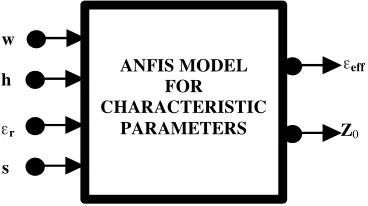
4. APPLICATION OF ANFIS TO THE COMPUTATION OF THE EFFECTIVE PERMITTIVITY AND THE CHARACTERISTIC IMPEDANCE

ANFIS MODEL FOR CHARACTERISTIC

PARAMETERS

h eff

r

w

Z0

s

ε

ε

Figure3. ANFIS model for the effective permittivity and the characteristic impedance computation of MCS line.

h, εr, s) and corresponding computed values (εeff orZo). Differences

between the target output (εeff or Zo) and the actual output of the

ANFIS are evaluated by the hybrid learning algorithm. The adaptation is carried out after the presentation of each set (w, h, εr, s) until the calculation accuracy of the ANFIS is deemed satisfactory according to some criterion (for example, when the error between the target output and the actual output for all the training set falls below a given threshold) or when the maximum allowable number of epochs is reached. The number of epoch is 2 for training. The number of MFs for the input variables w, h, εr, and s are 3, 3, 3, and 6, respectively. The number of rules is then 162 (3×3×3×6 = 162). The MFs for the input variables w, h, εr, and s are the triangular, generalized bell, gaussian, and gaussian, respectively. It is clear from Eq. (8) that the triangular, generalized bell, and gaussian MFs are specified by three, three, and two parameters, respectively. Therefore, the ANFIS used here contains a total of 846 fitting parameters, of which 36 (3×3 + 3×3 + 3×2 + 6×2 = 36) are the premise parameters and 810 (162×5 = 810) are the consequent parameters.

It is well known that the ANFIS has one output. For this reason, in this paper two separate ANFISs with identical structure are used for computing the effective permittivity and the characteristic impedance. Although the number of the inputs, the input values, the number of the MFs, and the types of MFs are the same for each ANFIS, the values of the premise and the consequent parameters for each ANFIS are different.

5. RESULTS AND CONCLUSION

The average absolute errors in training are 0.00140 and 0.31039 Ω, and in test are 0.00102 and 0.26994 Ω for both the effective permittivity and the characteristic impedance, respectively. In order to verify the validity and accuracy of the method proposed in this paper, the ANFIS results for the effective permittivity and the characteristic impedance of MCS line are compared with the experimental [2], theoretical [1, 3], and ANN results [4] in Table 1. It can be clearly seen from Table 1 that the results of ANFIS model proposed in this paper are in very good agreement with the results presented in [1–4].

Table1. Comparison of the experimental [2], theoretical [1, 3], ANN [4], and ANFIS results for the effective permittivity and the characteristic impedance of MCS line with h = 400µm, εr = 10.1,

s= 296µm, 95µm, 46µm, and w= 375µm, 374µm.

Parameters Experimental Results [2] RBDM [1] CMM [3] ANN [4] Present ANFIS Method

s= 296µm

w= 375µm

Z0 = 4 8.28

eff = 6 .47

Z0 = 4 7.52

eff = 6 .38

Z0= 4 9.90

eff = 6 .78

Z0 = 4 9.45

eff = 6 .77

Z0= 4 9.96

eff = 6 .78

s= 9 5µm

w= 374µm

Z0 = 4 3.05

eff = 6 .35

Z0 = 4 2.26

eff = 6 .07

Z0= 4 4.17

eff = 6 .44

Z0 = 4 4.41

eff = 6 .43

Z0= 4 4.21

eff = 6 .43

s= 4 6µm

w= 374µm

Z0 = 4 0.06

eff = 6 .28

Z0 = 3 8.25

eff = 5 .89

Z0= 4 0.06

eff = 6 .30

Z0 = 3 9.98

eff = 6 .28

Z0= 4 0.04

eff = 6 .30

Ω ε Ω Ω Ω Ω Ω Ω Ω Ω Ω Ω Ω Ω Ω Ω ε ε ε ε ε ε ε ε ε ε ε ε ε ε

The effective permittivity and the characteristic impedance test results of ANFIS model are compared with the results of CMM [3] in Figure 4. It is clear from Figure 4 that the results of ANFIS model proposed in this paper for the effective permittivity and the characteristic impedance of MCS are in very good agreement with the results of CMM. This very good agreement supports the validity of the neuro-fuzzy model and also illustrates the superiority of ANFIS.

70 140 210 280 350 420 490 560 630 5.5

6 6.5

7

Effective Permittivity

w

(a) The effective permittivity εeff.

70 140 210 280 350 420 490 560 630 30

40 50 60 70 80

90Characteristics Impedance

w

(b) The characteristic impedance Z0(Ω).

ANFIS CMM [3]

h= 400µm εr= 9.9

s= 46µm ♦

s= 144µm s= 192µm

set values for training.

As a consequence, a method based on the ANFIS for computing the effective permittivity and the characteristic impedance of MCS line is presented. The optimal values of premise parameters and consequent parameters are obtained by the hybrid learning algorithm. The results of ANFIS exhibit a good agreement with the experimental results. The proposed method is not limited to the calculation of the effective permittivity and the characteristic impedance of MCS line. We emphasize that this method can easily be applied to other microwave circuit problems.

REFERENCES

1. Yamashita, E., K. R. Li, and Y. Suzuki, “Characterization method and simple design formulas of MCS lines proposed for MMIC’s,”

IEEE Transaction on Microwave Theory and Techniques, Vol. 35, No. 12, 1355–1362, 1987.

2. Qian, Y. and E. Yamashita, “Additional approximate formulas and experimental data on micro-coplanar striplines,” IEEE Transaction on Microwave Theory and Techniques, Vol. 38, No. 4, 443–445, 1990.

3. Tan, K. W. and S. Uysal, “Analysis and design of conductor-backed coplanar waveguide lines using conformal mapping techniques and their application to end-coupled filters,” IEICE Transactions on Electronics, Vol. 82, No. 7, 1999.

4. Sagiroglu, S. and C. Yildiz, “A multilayered perceptron neural network for a micro-coplanar strip line,”Electromagnetics, Vol. 22, 553–563, 2002.

5. Jang, J.-S. R., “ANFIS: Adaptive-network-based fuzzy inference system,” IEEE Transaction on System, Man and Cybernetics, Vol. 23, 665–668, 1993.

6. Jang, J.-S. R., C. T. Sun, and E. Mizutani,Neuro-Fuzzy and Soft Computing: A Computational Approach to Learning and Machine Intelligence, Prentice-Hall, Upper Saddle River, NJ, 1997.

7. Guney, K. and N. Sarikaya, “Adaptive neuro-fuzzy inference system for the input resistance computation of rectangular microstrip antennas with thin and thick substrates,” Journal of Electromagnetic Waves and Applications, Vol. 18, No. 1, 23–39, 2004.

neuro-fuzzy inference system,” International Journal of RF and Microwave Computer-Aided Engineering, Vol. 14, 134–143, 2004. 9. Guney, K. and N. Sarikaya, “Input resistance calculation for circular microstrip antennas using adaptive neuro-fuzzy inference system,”International Journal of Infrared and Millimeter Waves, Vol. 25, 703–716, 2004.

10. Turkmen, I. and K. Guney, “Tabu search tracker with adaptive neuro-fuzzy inference system for multiple target tracking,”

Progress In Electromagnetics Research, Vol. 65, 169–185, 2006. 11. Daldaban, F., N. Ustkoyuncu, and K. Guney, “Phase inductance

estimation for switched reluctance motor using adaptive neuro-fuzzy inference system,” Energy Conversion and Management, Vol. 47, 485–493, 2006.