Title Page
Graph-embedding Enhanced Attention Adversarial Autoencoder
by
Yurong Chen
Bachelor of Science, Changsha University of Science & Technology, 2019
Submitted to the Graduate Faculty of the Swanson School of Engineering in partial fulfillment
of the requirements for the degree of Master of Science
University of Pittsburgh 2020
Committee Page
UNIVERSITY OF PITTSBURGH SWANSON SCHOOL OF ENGINEERING
This thesis was presented by
Yurong Chen
It was defended on March 31, 2020 and approved by
Liang Zhan, Ph.D., Assistant Professor, Department of Electrical and Computer Engineering Feng Xiong, Ph.D., Assistant Professor, Department of Electrical and Computer Engineering Jingtong Hu, Ph.D., Assistant Professor, Department of Electrical and Computer Engineering Thesis Advisor: Liang Zhan, Ph.D., Assistant Professor, Department of Electrical and Computer Engineering
Copyright © by Yurong Chen 2020
Abs tract
Graph-embedding Enhanced Attention Adversarial Autoencoder
Yurong Chen, MS University of Pittsburgh, 2020
When dealing with the graph data in real problems, only part of the nodes in the graph are labeled and the rest are not. A core problem is how to use this information to extend the labeling so that all nodes are assigned a label (or labels). Intuitively we can learn the patterns (or extract some representations) from those labeled nodes and then apply the patterns to determine the membership for those unknown nodes. A majority of previous related studies focus on extracting the local information representations and may suffer from lack of additional constraints which are necessary for improving the robustness of representation. In this work, we presented Graph-embedding enhanced attention Adversarial Autoencoder Networks (Great AAN), a new scalable generalized framework for graph-structured data representation learning and node classification. In our framework, we firstly introduce the attention layers and provide insights on the self-attention mechanism with multi-heads. Moreover, the shortest path length between nodes is incorporated into the self-attention mechanism to enhance the embedding of the node’s structural spatial information. Then a generative adversarial autoencoder is proposed to encode both global and local information and enhance the robustness of the embedded data distribution. Due to the scalability of our approach, it has efficient and various applications, including node classification, a recommendation system, and graph link prediction. We applied this Great AAN on multiple datasets (including PPI, Cora, Citeseer, Pubmed and Alipay) from social science and biomedical science. The experimental results demonstrated that our new framework significantly outperforms several popular methods.
Table of Contents
Preface ... viii
1.0 Introduction ... 1
2.0 Related Work ... 5
2.1.1 Graph Embedding ... 5
2.1.2 Shortest Path Length for Graph Learning ... 6
2.1.3 Adversarial Networks on Graph Embedding ... 7
3.0 Great ANN Architecture ... 8
3.1.1 Graph Shortest Path Length Attention Layer (GSA) ... 8
3.1.2 Enhanced Attention Autoencoder ... 12
3.1.3 Adversarial Networks for Graph Learning ... 16
4.0 Experiments ... 20 4.1.1 Datasets ... 20 4.1.2 Parameter Settings ... 21 4.1.3 Results ... 23 5.0 Conclusion ... 25 Bibliography ... 26
List of Tables
Table 1 Summary of the datasets ... 21
Table 2 Summary of testing Micro-F1 results on PPI in the inductive setting. ... 24 Table 3 Summary of testing results on Cora, Citeseer, Pubmed and Alipay in the
transductive setting ... 24 Table 4 Hyper-parameters analysis of the shortest path length ... 24
List of Figures
Figure 1 The main process of the Great AAN ... 4
Figure 2 The Graph Shortest Path Length Attention Layer. ... 9
Figure 3 The Multi-Heads Attention Mechanism ... 11
Preface
This basis for this research is for developing better methods of research about graph-structured network like social science and biomedical science network. As the world moves further into the digital age, and with the rapid growth of emerging applications such as social network analysis, Web semantic analysis, bioinformatics network analysis, and traffic navigation, large-scale graph data with large large-scales, complex internal structures, and diverse have appeared. In our research, we study the better methods for representation those larger graph datasets and have proved our methods archived great performance.
In the end, I cannot have achieved my current success without strong supports. First of all, my parents and family, who supported me with love and understanding. And secondly, my advisor, Professor Zhan who give me lots of guidance and direction during my research. And he encouraged me when I face difficult. Also, thanks for my committee members, each of whom has provided patient advice and guidance throughout the research process. Thank you all for your support.
1.0 Introduction
Low-dimensional vector embeddings of nodes in the large social networks have proved quite useful as feature inputs for various graph analysis tasks. The low-dimensional embedding meaningful vector of nodes which can capture and preserve the network structure has attracted great researchers’ attention. The key idea of node embedding methods is to distill high dimensional sparse data vector into a useful dense vector. With the reduced dimensionality, various graph analysis tasks can be conducted efficiently, such as node classification [1], link prediction [2], knowledge graph representation [3] and biological networks [4] or brain connectomes classification [5] node clustering [6].
In the past decades, the most common practical methods for graph embedding are Locally Linear Embedding [7], which assume one node can be represented by the linear combination of its neighborhoods and to minimize the loss of real data value and the linear combination value; Laplacian Eigenmaps [8], which proposed that the nodes which have high similarity (measure by the edge) should be homologous in the embedding space domain so that the cost function is the edge weight multiplying the difference of two nodes; And Graph Factorization [9], which achieved graph embedding via matrix factorization. Since the underlying network structure is complex with high dimensional data information, those traditional methods cannot capture the non-linear the node features and network structure and preserve the global and local node information.
However, those traditional algorithms face the challenge when embedding non-linear node features and lack the ability to deal with sparse high dimensional information. Based on the previous graph work and introducing some concept of work2vec, Deepwalk [10] adopted a random
walk to construct the “sentence sequence” of a node, in that way, the embedding features which provide the “symbiotic relationship” of nodes can be formed by the Deepwalk sentence. Unlike Depth First Search (DFS) random walk of Deepwalk, LINE [11] is proposed to respectively optimize the first order proximity and second-order proximity via Breadth-First Search (BFS). Based on this, node2vec [12] combined BFS with DFS for considering both local information from BFS and global structure information from DFS achieved successful results.
In recent years, with the development of deep learning, researchers explored deep learning algorithms to make up for deficiencies of previous shallow-level methods. SDNE [13] proposed deep autoencoder to learn embedding of the graph adjacent matrix to preserve both global structure and local structure. Other than unsupervised graph embedding learning methods, Graph Convolutional Neural Network (GCN) [14] is one of the most significant milestones. Based on the huge successful application of convolutional neural networks (CNNs) on grid-like structure data, GCN achieved generalizing convolutions on graph domain. In conclusion, GCN is categorized as spectral domain methods and non-spectral domain methods. On the spectral approaches, the key idea is the convolutional transform computed by the eigendecomposition of the graph Laplacian on the Fourier domain. Depend on this, the spectral convolutional neural networks [15] are proposed based on the spectrum of the graph Laplacian. However, the high complexity, lack of spatial localization motivated the second-generation Spectral Convolution [16] adopting Chebyshev expansion and the third generation Spectral Convolution network [17] increased the depth of layer with decreasing the breath of layer. Although the complexity and computational cost are reduced, the need for eigendecomposition and spatial limitations impeded spectral approaches to be a generalized framework on different datasets. On the other hand, non-spectral
algorithms have to be addressed the problem that the nodes in the graph have different numbers of neighbors. Learning Convolutional Neural Networks for Graphs (CNN4G) [18] selected particular nodes via centrality and assigned them specific features number, then adopted convolutional operation on the constructed matrix. Moreover, GraphSAGE [19] for computing node representations in an inductive manner can operate by sampling neighborhoods of each node and then feeding them through a recurrent neural network.
Nowadays, the attention mechanism attracted lots of attention [20][21] due to its highly efficient learning ability. Graph Attention Networks (GATs) [22] dynamically computed the hidden representations of each node in the graph and stacked a multi GAT layer to get a larger receptive field. Although its’ results on several datasets proved it is state-of-the-art methods, it only focuses on first order proximity and lack of second-order proximity so that it cannot represent node global structure information and only count those directly connected nodes which make lack those structurally connected nodes impact.
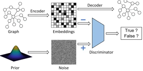
Inspired by those recent work, we proposed an end-to-end graph-embedding enhanced attention adversarial autoencoder networks as Figure 1 shown. The idea is that firstly compute the latent representations of each node via graph attention networks with multi- heads self-attention strategy combined shortest path length coefficient; secondly, based on the embedding vectors, we build two parallel decoder architecture networks: one is for minimizing the difference between decoder vectors and the node features, anther is for minimizing the difference between decoder vectors and the node adjacency matrix; In the end, the adversarial network is designed to discriminate the real data (the noise data with prior distribution) and the fake data (the generated
embedded features by encoder). In our method, the first order proximity of the node-local information is learned by the modified GAT layers which can conduct on a query (Q) and a set of key (K) value (V) pairs to compute the output. The graph structural information and node global features are mapped though our constructed second-order proximity loss function of the autoencoder. Moreover, for improving the features data distribution network structural information, the adversarial game is used to tuned embedded feature vectors with a data distribution that we can as the prior data distribution. After the latent representation matches the prior distribution, the decoder of the autoencoder is trained to map the imposed prior to the data distribution which enhanced the model representation robustness against uncertainty.
Figure 1: The main process of theGreat AAN consisting of two parts: (1) on the top line, the autoencoder for node features embedding; (2) on the bottom line, the adversarial network for embedding representation data distribution learning.
2.0 Related Work
Related works mainly consist of three categories: Algorithms for graphs embedding, applications of shortest path length for graph learning, and applying adversarial networks on graph embedding. Each will be discussed below and compared with our proposed model.
2.1.1 Graph Embedding
As mentioned in the introduction, there are many effective graph embedding algorithms and can mainly be divided into two categories: random walk based methods and deep learning-based methods. For the random walk learning-based methods, Deepwalk [10] is introduced to preserves higher-order proximity with node sequences by maximizing the likelihood 𝒍𝒐𝒈𝑷𝒓 = {𝑣𝑖−𝑘, … , ℎ𝑖−1, ℎ𝑖+1, … , ℎ𝑖+𝑘|𝑌𝑖}, here 2𝑘 + 1 is the length of the random walk. Similar to DeepWalk, LINE [11] and node2vec [12] produce higher-quality and more informative embedding representations. Hierarchical representation learning for networks (HARP) [23] proposed another algorithm with aggregating previous layers’ nodes using graph coarsening to improve the local optima. Recently, Discriminative Deep Random Walk (DDRW) [24] extended the random walk technique to learn the network structure and node attributes and achieved great performance. ON the other hand, deep learning-based methods have grown rapidly due to its high performance on graph-related tasks. SDNE [13] and DNGR [25] firstly introduced deep autoencoder to generate non-linear embeddings. Then GCN [14] is proposed to reduce the computationally cost and for larger sparse graph networks. Recently, Deep Attributed Network Embedding [26] designed a
novel deep attributed network embedding approach which can preserve various proximities in both node attributes and topological structure. And via introducing the attention mechanism, GAT [22] addressed several key challenges in graph neural networks. In our paper, based on GAT, we adopt the shortest path length to preserve more structural spatial information in the graph and the details will be explained in the next section.
2.1.2 Shortest Path Length for Graph Learning
Most previous graph learning works focus on the 1st-order or 2nd-order proximity. The 1st-order proximity considers those nodes with the only direct connection that should be embedded closely while the 2nd-order proximity will translate those nodes sharing with the same neighborhoods using similar embedding representations. However, some studies on the shortest path length between nodes demonstrated that the shortest path length can be one of the most important measures to quantify the relationship among nodes [27]. For example, Path length associated community estimation (PLACE) [28] has been proposed to estimate the modular structure for brain structural networks by differentiating the difference between nodes using the shortest path length. Especially in the larger graph-structure network, the shortest path length provides a different way to quantify the distances between pair of nodes [29]. In this paper, by including the Shortest Path length into our graph attention layer, we can explore more higher-order node information to preserve global and local node structure with more precious and robustness.
2.1.3 Adversarial Networks on Graph Embedding
Recently, Generative Adversarial Network (GAN) [30] has attracted a lot of attention because of its huge success in various applications such as word sequence generation [31] and graph representation learning [32]. GAN [30] plays an important role in deep learning which can be formulated as a minimax adversarial game. This minimax adversarial game consists of a generator and a discriminator. Due to the superior performance of GAN, Self-Paced Network Embedding [33] extended the sampling strategy to the generative adversarial network which can sample difficult negative nodes. Moreover, GraphGAN [34] tried to reconstruct the distribution of nodes’ underlying true connectivity, while the discriminator is trained to detect whether the sampled node is from the ground truth or generated. Unlike those aforementioned studies, WGAN [35] enhanced the training of the GAN network by introducing the minimizing the Wasserstein distance as the following:
𝑊(𝑃𝑟, 𝑃𝑔) = inf
𝛾~ ∏(𝑃𝑟,𝑃𝑔)𝔼(𝑥,𝑦)~𝛾[||𝑥 − 𝑦||] (1) between the prior data distribution (x) and the generator data distribution (y), which can let the embedded features from the generator be closer to the prior distribution. Based on this, Adversarial network embedding [36] aims to capture stable and robust latent feature representations with regularizing data distribution. In our paper, following with [36] where the goal of the generator is to map data samples from some prior distribution to data space, while the discriminator tries to differentiate fake samples from true data, we incorporate this component into our graph attention autoencoder showing.
3.0 GREAT AAN Architecture
In this section, we will present the graph shortest path length attention layer in Section 3.1, the autoencoder network in the section Section 3.2. And the adversarial mechanism network will be introduced in Section 3.3.
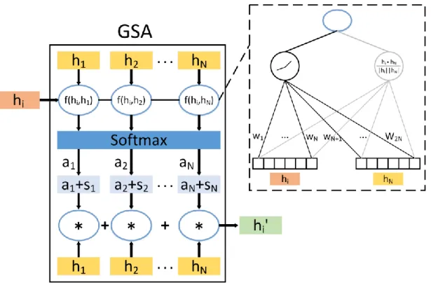
3.1.1 Graph Shortest Path Length Attention Layer (GSA)
The inputs of GSA block layers are a branch of nodes' features, 𝒉 = {ℎ1, ℎ2, … , ℎ𝑖, … , ℎ𝑁}, ℎ𝑖 𝜖 ℝ𝐹; nodes' corresponding adjacency vectors can be denoted as 𝒂 = {𝑎1, 𝑎2, … , 𝑎𝑖, … , 𝑎𝑁}, 𝑎𝑖 𝜖 ℝ𝑁 , and the shortest path length nodes' vectors 𝒔 = {𝑠1, 𝑠2, … , 𝑠𝑖, … , 𝑠𝑁}, 𝑠𝑖 𝜖 ℝ𝑁, where 𝑁 represents the number of nodes, and 𝐹 is the number of dimension of features of each node. The output of GSA is a new set of nodes embedding features, 𝒉′ = {ℎ
1′, ℎ2′, … , ℎ𝑖′, … , ℎ𝑁′}, ℎ𝑖′𝜖 ℝ𝐹 ′
where 𝐹′ can be any number of dimension of embedding features. The main graph attention layer follows the work of [20][22], and we particularly incorporate multiple shortest path lengths, from the Dijkstra's Shortest Path First algorithm [37] and Bellman–Ford algorithm [38] into the attention mechanism to improve (1) the node structural spatial information; (2) network global information representation; (3) the robustness of graph structural representations.
In order to project the high dimensional sparse features data into a meaningful expressive manifold space and prepare for the downstream multi-heads attention strategy on the multi embedding sub-spaces, the weight matrix for linear transformation, 𝑊𝐾 𝜖 ℝ𝐹′× ℝ𝐹 is adopted on
Figure 2: The Graph Shortest Path Length Attention Layer. 𝒉𝒊 represents the input node features. The
function 𝒇 (𝒉𝒊, 𝒉𝑵) consists of the average of the cosine similarity (gray line) and one LeakReLU activation function (black line). The output node feature vector 𝒉𝒊′ will be the sum of all nodes’contributing weights
generated by our similarity matrices.
α, instead of normal processes that take their dot product and using SoftMax to normalize, both fully connected layer and cosine similarity are adopted, and the resulted output vectors are concatenated as the output of attention coefficients α. In this process, the transformed features of each node are taken as the query to match others for retrieval of the similarity of the query node and other nodes. And then the weighted sum is the similarity coefficient with the value that in the self-attention and the value is the same as the key. For one single node, this operation is shown as the following:
{ 𝑓(ℎ𝑖, ℎ𝑁) =1 2(𝐹𝐶(ℎ𝑖, ℎ𝑁) + 𝐶𝑜𝑠𝑖𝑛𝑒(ℎ𝑖, ℎ𝑁)), 𝛼𝑖 = 𝑆𝑜𝑓𝑡𝑚𝑎𝑥(𝑓(ℎ𝑖, ℎ𝑁)), ℎ𝑖′= ∑(𝛼𝑖 ℎ𝑖) 𝑁 𝑛=1 (2)
For avoiding the inaccuracy caused by “Curse of Dimensionality” [3] of computing the similarity coefficient using single dot product or cosine operation and uninterpretability using neural perceptron, in this paper, we take the average of the output of perceptron and modified cosine similarity.
One important issue in previous works is that they only compute the αi for those nodes that are neighbors in the adjacency matrix of the query node. In other words, only those directly connected nodes are computed in the attention layer. However, due to the sparse, there are a few nodes connected with each other and just sticking to count the first-order information of the node would lead to the loss of many correlations or information form indirectly connected nodes, which also preserve important implications. Motivated by this, we proposed a novel shortest path length attention mechanism based normal self-attention layer for ameliorating those mentioned problems. The main process is shown in Figure 2.
It's worth noting that the introduction of the shortest path length leads to two changes: the first one is the extra calculation of the attention coefficients for those indirectly connected nodes as taking considering of 𝑠𝑖 in Figure 2; another modification is that the attention coefficient 𝑎𝑖 is combined with the original attention coefficient 𝑎𝑖 and the normalized shortest path length 𝑠𝑖 by
Path First algorithm [37] and Bellman-Ford algorithm [38] are adopted to computing the shortest path length between two nodes. Briefly, given a weighted graph network of 𝐺 = {𝐸, 𝑉} where 𝑉
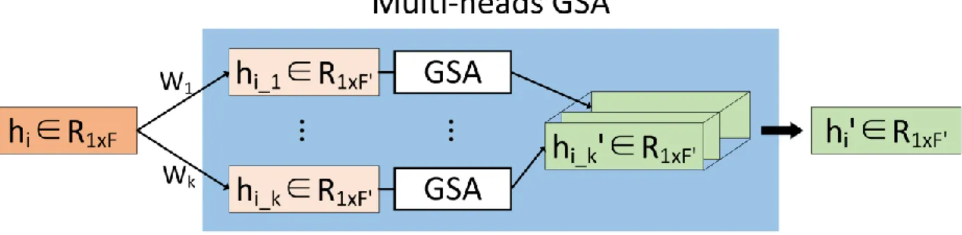
Figure 3: The Multi-Heads Attention Mechanism. 𝑾𝟏, 𝑾𝟐, … , 𝑾𝒌 represent the different feature transformation matrixes that can transform hi into 𝒉𝒊_𝟏, 𝒉𝒊_𝟐, … , 𝒉𝒊_𝒌 , which can consider different aspects node attention at each sub-space. Through our GSA layer, all output features vectors can be averaged or fed into a neural layer to get the final output node representation features hi.
represents all vertices (nodes) and 𝐸 denotes the set of edges, the output of the Dijkstra’s algorithm is the 𝑆𝐷 = [𝑠𝑖𝑗] 𝜖 ℝ𝑁×𝑁, where 𝑠
𝑖𝑗 is the shortest path length between node i and node j with Dijkstra's algorithm, Bellman-Ford proceeds by relaxation, that is the approximation of the correct distance is replaced by a better approximation until the final solution is reached and output 𝑆𝐵 = [𝑠𝑖𝑗] 𝜖 ℝ𝑁×𝑁, and in the result section, we will discuss the different results of the rate of weights of shortest path length.
Moreover, considering the information from different embedding representations may comprehensively pay attention to different aspects of the information, the multi-head attention strategy is adopted to stabilize the training process and provide more robust results. Figure 3 shows the execution processes, where 𝐾 is the number of independent different transformations. Each node features at different sub-space will be taken as the input of the self-attention layer mentioned
before to get the attention coefficient. Then the final attention coefficient is computed by one fully connected layer that concatenates all individual attention coefficients. Lastly, we will apply the nonlinear activation function LeakyReLU (with negative slope 𝑎 = 0.2) as follows:
ℎ𝑖′= 𝑀𝑢𝑙𝑡𝑖𝐻𝑒𝑎𝑑(ℎ𝑖, ℎ𝑁) = 𝐿𝑒𝑎𝑘𝑅𝑒𝐿𝑈 (𝐶𝑜𝑛𝑐𝑎𝑡(ℎ𝑖𝑘)). (3) To sum up, each embedded node features ℎ𝑖′ in GSA is calculated by the multi-head transformation of original node features ℎ𝑖 with a query-retrieval self-attention layer incorporated with shortest path length, and the cross-entropy loss function is adopted for the classification during the encoder training and for regularizing the data which can enforce the embedding node vectors be closer in the hidden space to preserve the first order proximity. The final encoder loss function is shown as follows:
𝐿𝑜𝑠𝑠𝐸𝑛𝑐𝑜𝑑𝑒𝑟 = 𝐿𝑜𝑠𝑠𝐶𝑟𝑜𝑠𝑠𝐸𝑛𝑡𝑟𝑜𝑝𝑦 + 𝐿𝑜𝑠𝑠1𝑠𝑡 , 𝐿𝑜𝑠𝑠𝐶𝑟𝑜𝑠𝑠𝐸𝑛𝑡𝑟𝑜𝑝𝑦 = ∑𝑁𝑖=1(𝐿𝑎𝑏𝑒𝑙𝑖)log (𝑦𝑖) , (4) 𝐿𝑜𝑠𝑠1𝑠𝑡 = ∑ ||𝑦𝑖− 𝑦𝑗|| 2 2 = 2𝑡𝑟𝑎𝑐𝑒(𝑌𝑇 𝐿 𝑌) 𝑁 𝑖,𝑗=1 .
where 𝑦𝑖 is the embedding representation of 𝑛𝑜𝑑𝑒𝑖 , 𝑌 is the embedding graph and 𝐿 is the Laplacian Eigenmaps.
3.1.2 Enhanced Attention Autoencoder
Although existing methods [11][12][22] did the node classification task based on the embedding features and achieved remarkable results, those studies built the network only focusing on the encoder network and ignored the decoder part. Due to the excellent performance, the autoencoder becomes more and more popular on the graph embedding tasks. However, in previous
works [13], the fully connected layer is the prior option to build the autoencoder. Although it can achieve satisfying performance in some certain cases, it is hampered by carefully-crafted the number of layers and/or the number of neural cells.
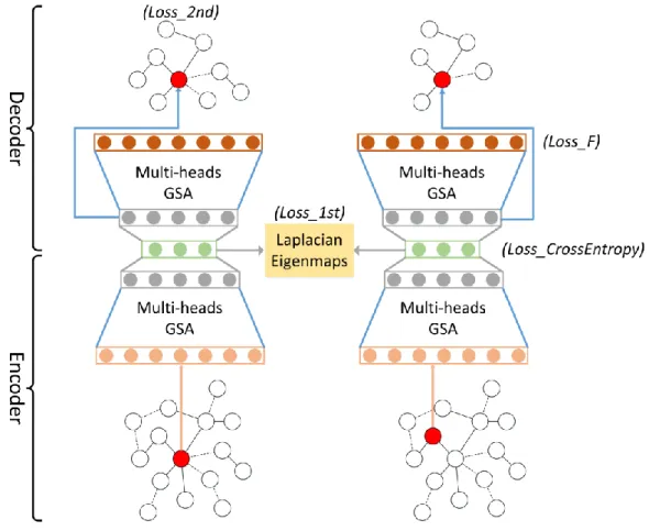
Apparently, another issue is that only the first order proximity will be optimized to make two nodes closer in the embedding manifold space when there is a high similarity in the raw data space. However, the first order proximity is not enough, and the second order proximity is also crucial [11], because it represents the similarity of two nodes’ neighbor sets. So that it can help the model to learn more local and global structure information and improve the robustness to the sparse network which results from embedding two nodes closer when their neighbors’ sets are similar. Considering this and for better model generalization, we propose a novel autoencoder attention network. The encoder part adopts the GSA layer as described in Section 3.1, in this section, we will focus on the decoder part.
As we mentioned before, given the node features of the graph to the encoder part, the output will be the features representations for each node. Taken the outputs of the encoder as the inputs of decoder, we built two parallel decoder networks: the first one is for reconstructing the node neighborhood’s relationship which is the graph adjacency matrix and the second one is to conjecture the node features. Both decoder networks are stacked by our GSA layers. Similar to the architecture in the encoder, two graph attention layer blocks are adopted. The purpose of the first layer is to project the linear transformation of the embedded features into the hidden space. For the feature decoder network, the dimension of hidden features is 1 × 𝐹 where 𝐹 is the original dimension of node features; After that, another independent layer is followed. In the feature decoder network, it is the self-attention query-retrieval layer for minimizing the difference of the
data distribution between the real data and the reconstructed data. Also, in this layer the multi- head method is adopted with the same number of 𝐾 used in the encoder GSA layers. The normal loss function used in previous work is the Kullback–Leibler (𝐾𝐿) divergence for decoding same data distribution as following:
𝐷𝐾𝐿(𝑝||𝑞) = ∑ 𝑝(ℎ𝑖)𝑙𝑜𝑔𝑝(ℎ𝑖) 𝑞(ℎ𝑖) , 𝑁
𝑖=1
(5) where 𝑝(ℎ𝑖) represents the true features of data distribution while the 𝑞(ℎ𝑖) is the modeling features data distribution. In order to achieve a data distribution 𝑞(ℎ𝑖) that is the closest to 𝑝(ℎ𝑖), we can minimize the 𝐾𝐿 divergence information gain. However, it is hard to converge at the low dimensional embedding space and easy to cause simplifying problems in generating the samples. In detail, the 𝐾𝐿 divergence tends to infinity when there is no overlap between two distributions and has a mutation when states from non-overlap to overlap. One alternative solution to avoid this issue is to adopt the Wasserstein distance (Equation 1) as the loss function [35]. Unlike 𝐾𝐿 divergence, the Wasserstein distance can provide smoothing useful gradient even there is no overlap between two distributions. Based on the Equation 1 that for ∏(𝑃𝑟, 𝑃𝑔) each marginal distribution is 𝑃𝑟 or 𝑃𝑔 and for each joint probability distribution 𝛾 of true sample 𝑥 and generating sample 𝑦, we want to minimize the lower bound of the expected value of distance. So, the features decoder loss function is defined as following:
𝐿𝑜𝑠𝑠𝐹 = 1
𝑁∑(𝔼ℎ𝑖~𝑝(ℎ) − 𝔼ℎ𝑖′~𝑝(ℎ′)) , 𝑁
𝑖=1
(6)
where ℎ𝑖is the input node features and ℎ𝑖′ is the output reconstructed node features of autoencoder.
vector to preserve the network structural spatial information, the second layer of another network of decoder is built to recover the graph adjacency matrix using the self-attention transfer. And for this decoder network, the dimension of the hidden features is 1 × 𝑁 where 𝑁 is the number of
Figure 4: The Enhanced Attention Autoencoder. Each node features would be fed into the autoencoder whose parameters are shared. In the encoder part, the loss function includes CrossEntropy function that can map node features into right classes and the first order proximity loss function which can guarantee connected nodes will be mapped closer. And in the decoder network, we minimize data distribution of reconstructed node features and the second order proximity which can ensure those node embedded closer when they share with the same neighborhood relationship.
nodes. The detailed architecture of the combined autoencoder network is shown in Figure 4. Beside reducing the common mean square loss (MSL) of the data, the zero may take the dominating part
in each adjacency matrix for some sparse graph cases. In those cases, the model can easily achieve the optimal solution but hard to use a gradient descent method to optimize the mean square error loss function with given output all zero. Inspired by the loss function of SDNE, the penalty coefficient 𝛽 is used to control the zero elements. More minutely, if there is no connection between 𝑛𝑜𝑑𝑒𝑖 and 𝑛𝑜𝑑𝑒𝑗, 𝛽 equals to 1. Else, 𝛽 is set to larger than 1. In the end, the loss function of second order proximity preserving with adjacency decoder as shown in the following equation:
𝐿𝑜𝑠𝑠2𝑛𝑑 = ∑ ||(𝑎𝑖𝑗− 𝑎𝑖𝑗′)𝛽𝑖𝑗|| 2 2 𝑁 𝑖,𝑗=1 , (7) Where 𝑎𝑖𝑗′ represents the value of two nodes’ reconstructed adjacency matrix, 𝛽𝑖𝑗 is the correspond penalty coefficient. With minimizing this loss function, the nodes which have similar neighborhood structure are embedded near in the representations space.
In conclusion, the first order proximity is guaranteed by the encoder network to preserve the local structural node information which map the vertexes near which have multi edges between them. And the second order proximity can keep the global network structure by reconstructing the neighborhood set of vertexes. The final loss function will jointly encoder part and decoder part as following:
𝐿𝑜𝑠𝑠_𝐴𝐸 = 𝐿𝑜𝑠𝑠_𝐸𝑛𝑐𝑜𝑑𝑒𝑟 + 𝐿𝑜𝑠𝑠_𝐷𝑒𝑐𝑜𝑑𝑒𝑟, (8) 𝐿𝑜𝑠𝑠𝐷𝑒𝑐𝑜𝑑𝑒𝑟 = 𝐿𝑜𝑠𝑠𝐹+ 𝐿𝑜𝑠𝑠2𝑛𝑑.
3.1.3 Adversarial Networks for Graph Learning
The most impactful framework that introducing GAN into the graph learning is the GraphGAN [34], which training the generator 𝐺 to the distribution of neighborhoods of one node that try to cheat the discriminator; on the other hand, the discriminator is honed to differentiate between the real node and the generated node. Different from common GAN, Adversarial Network Embedding [36] conducts the adversarial idea on the graph tasks that train the generated data distribution closer to the prior data distribution in order to regularize the representation features. Due to the simple network structure of the normal graph embedding network, it is difficult to preserve the node information comprehensively and robustly, which only receives very little attention in the graph research. Motivated by the great performance of Adversarial Network Embedding, we introduce the idea of the adversarial network into our method. The idea of the adversarial network is incorporated with the autoencoder. Specifically, the generator (𝐺) is played by the encoder part of autoencoder, which tries to represent a serious of non-linear attention transformations of the input sparse high dimensional features into embedding features. The discriminator (𝐷) is designed with a 1-dimension convolution layer and the fully connected layer which aims to differentiate the embedding features from the valid data which the sample possesses at the set prior distribution. The detailed network layer is shown in the bottom part of Figure 1, and in the training process, the alternative update strategy is used to train the autoencoder network and the discriminator. The generator optimization is provided in the previous section, therefore, in the last section, we will only focus on discriminator optimization. This training process can be treated as a two-player minimax game with the discriminator and generator playing against each other. After optimization, the generator (the encoder of autoencoder) aims to embed features vector with the target distribution.
In our framework, given the valid samples from the prior distribution 𝑝(𝑧) data, while fake samples are embedded feature vectors from the encoder generator as the inputs, the goal for discriminator is to tell apart the prior distribution valid data from the fake data of embedded vectors. Selecting a proper prior distribution is the most significant step during the adversarial training. Like previous work in graph GANs research [40], the data prior distribution is commonly defined as Gaussian noise or Uniform noise which helps autoencoder network to learn useful and
robust embedding representations against uncertainty. In our experiments, we test those two prior data distributions and show almost have the same impact on results. However, here we only proposed a generalized framework that other researchers can further used with their particular data distribution which can enhance the application applied task performance. The detailed network layers are built by three fully connected layers, the front two layers are both set with 𝑁 neural cells and the final layer is set with 1 neural cell which makes a distinction between the valid samples and fake samples. The solution to this training process of discriminator can be expressed as following:
The encoder is trained to minimize the second term in order to camouflage its output as prior samples.
In conclusion, we propose an end-to-end adversarial autoencoder graph shortest path length attention network for node classification and graph embedding combined with supervised and unsupervised learning. The GAN-like network is introduced with the autoencoder as generator whose loss function is 𝐿𝑜𝑠𝑠𝐴𝐸 in Equation 8 and the neural network as discriminator whose loss function is the Equation 9. In the training process, the alternative updating weights strategy is used for finally achieving the steady model in two stages: (1) Train the autoencoder to fool the discriminator with its generated embedding node representations. (2) Train the discriminator to distinguish the true samples data distribution from the fake samples generated by the autoencoder.
4.0 Experiment
We have conducted on the multi evaluation of the Great AAN model against various strong and performance baselines and previous works, on one inductive task and four prevalent graph-based benchmark transductive tasks, achieving or surpassing sota performance across all of them. The following section will provide datasets, our experimental set-up details, results, and qualitative analysis of Great AAN compared with others.
4.1.1 Datasets
Transductive learning: Three standard citation network benchmark datasets— Citeseer, Cora, Pubmed [42] and one account-device network Alipay [43]. In those three citation datasets, documents are treated as nodes and the citation links correspond to undirected edges. The datasets include elements of a bag-of-words feature vectors representation for each document and all citation links between documents. It is usually that only using 20 labeled samples per class to train the model and evaluating on 1000 or 1500 test nodes. The Citeseer dataset includes 3327 documents, 4732 citation links, 6 classes and 3703 features for each node. The Cora dataset contains 2708 documents, 5429 citation links, 7 classes and 1433 features per node. The Pubmed dataset contains 19717 documents, 44338 citation links, 3 classes and 500 features per node as shown in Table 1. And the Alipay dataset is built for detecting malicious accounts in the online payment. The nodes represent the users’ accounts. The edges mean the login relationships between accounts and their using devices during a period. Discretization of login behaviors into hours and account profiles treated as node features. The class labels consist of malicious accounts and normal
accounts. This dataset includes 981748 nodes, 2308614 edges and 4000 features per node. Inductive learning: For the graph leaning task on biological networks, we make use of a protein-protein interaction (PPI) dataset [41] for multi-label node classification. The dataset contains 24 graphs with 20 graphs for training, 2 for validation and 2 for testing. And each graph represents a different human tissue with each node corresponds a protein and edges mean the interaction between proteins. Each protein has input 50 features that include of positional gene sets, motif gene sets and immunological signatures and 121gene ontology sets as labels. The average number of nodes per graph is 2372 as shown in Table 1. The goal is to predict which labels are contained in each node.
4.1.2 Parameter Settings
For the encoder part, a two-layer graph shortest path length attentional layer is adopted. The first layer includes a set of a linear transformation with 𝐹′= 128 and 6-heads graph shortest path length attentional layer for a total output with 768 features with leaky ReLU activations (with a leak of 0.2) and batch normalization (BN) [44]. Then a fully connect layer as the second layer is followed for node classification with transforming 768 hidden layer features to 𝑁 features where
𝑁 represents the number of the node classes. In the combination function of adjacency matrix weights and two shortest path length values, the weight of computed attention coefficient 𝜆𝛼 is 0.7 and both two shortest path length weights 𝜆𝑠 are 0.15. Also, we show the choosing different rate of 𝜆𝛼 and 𝜆𝑠 will make different results in Table 4. During the whole training process, the dropout layer [45] with 𝑝 = 0.5 is used to each layer for avoiding overfitting and λ = 0.001 is applied in the 𝐿2 regularization. Those parameters are all suitable inductive learning, but for transductive leaning, except the 𝐹′= 8 with 48 hidden features are different, other parameters are the same. Also, Adam optimizer with an initial learning rate of 0.005 for all datasets. For the decoder part, the same structure as the encoder is applied with a two-layer graph shortest path length attentional layer which the first layer consists of a linear transformation with 𝐹′ = 128. And then followed by the fully connected layer with output F features, where F represents the row feature dimension of the node. Also, anther fully connected layer for reconstructed the neighborhood relationship via adjacency matrix transfers hidden features to 𝑁 features where 𝑁 is the number of nodes. For the discriminator (𝐷) of the framework, the standard three neural layer network is applied, which consists of a 512-512-1 layer structure. For the first two layers, leaky ReLU activations (with the leak of 0.2) and batch normalization are also followed and the dropout layer with 𝑝 = 0.5. For the final output layer, the sigmoid activation function is used for classification. The prior distribution of adversarial learning is set to U [-1, 1] or N [-1, 1]. Finally, all training processes are conducted on NVIDIA Tesla P100 GPUs with the Pytorch framework.
4.1.3 Results
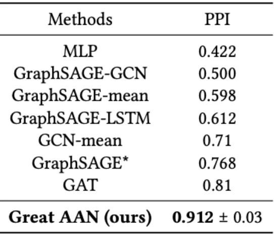
For the inductive task on the PPI dataset, we provided the 𝑚 − 𝐹1 score as the evaluation metric, which has an overall evaluation of precision and recall. Training on the nodes of the 20 graphs, 2 for validation and testing on 2 untrained graphs. We compared our Great AAN model with several baselines, such as MLP (multilayer perceptron), utilizes the node features but not the structures of the graph, and state-of-art models such as GraphSAGE [19]. GraphSAGE* represents the best GraphSAGE result we are able to obtain by just modifying its architecture. GCN [14] that “GCN-mean” by averaging the neighborhoods instead of GCN and GAT Table 2. The results obviously show the effectiveness and performance of graph attention autoencoder with the shortest path length connections and adversarial learning. More specifically, we are able to improve upon GAT by a margin of 0.102 on the PPI dataset demonstrating that our model has the potential to be applied in inductive settings. For the transudative learning task of node classification, the experiments conducted on several graph benchmark datasets including Cora, Citeseer, Pubmed and Alipay. The accuracy and F1 are reported on testing nodes. Comparing with nowadays state-of-the-art techniques such as DeepWalk, node2vec, ICA [46], Chebyshev, GCN, MoNet [47], GraphSAGE and GAT. We report the comparison results of transudative settings on those datasets in Table 3. In most cases, we found our method achieved or matched state-of-the-art results.
Furthermore, for analyzing the hyper-parameters weights of the shortest path length in of 𝜆𝑠. We changed each of 𝜆𝑠 and 𝜆𝑎 = (1 − 2 × 𝜆𝑠) to analyze the impact of joining the shortest path length with attention layer. The results are shown in Table. 4 and all these results are obtained from the Cora dataset. And as we can see, the best performance archived at 𝜆𝑠 equals 0.15 so that 𝜆𝑎 is 0.7.
Table 3: Summary of testing results on Cora, Citeseer, Pubmed and Alipay in the transductive setting. In accordance comparison and with former benchmarks, we report accuracy for Cora, Citeseer, Pubmed, and F1 for Alipay.
5.0 Conclusion
In this work, we presented a novel, generalized framework, graph-embedding enhanced attention adversarial autoencoder networks (Great AAN) for Social Network which focuses on studying the graph embedding features representation and applying the learned embedding features to address the node classification task. The Graph Shortest Path Length Attention Layer (GSA) improved assigning different significance to different nodes within a neighborhood even though there is no direct connection with preserving the structural shortest path length. Our network can copy with different sized neighborhoods of nodes, which does not rely on the whole graph structure, thus it can address many previous spectral-based approaches challenges. With the decoder network, we further address the problem of preserving structure information and sparsity by jointing the first order proximity and second-order proximity, so that the features of the learned representation can be local and global structure-preserving. A particularly interesting research GAN is taken as embedding features adversarial leaning with a prior data distribution to enhance the robustness. Finally, Our models have successfully achieved state-of-the-art performance across four well- established node classification benchmarks, both inductive task (PPI) and transductive task (Cora, Citeseer, Pubmed and Alipay).
Bibliography
[1] H. L. Jiliang Tang, “Node classification in signed social net- works,” 16th SIAM International Conference on Data Mining 2016, SDM 2016, pp. 54–62, 2016.
[2] G. P. Gao S, “Temporal link prediction by integrating content and structure information,” In CIKM, pp. 1169–1174, 2011.
[3] Y. Lin, “Learning entity and relation embeddings for knowledge graph completion,” Twenty-ninth AAAI conference on artificial intelligence, 2015.
[4] M. Zhang, “An end-to-end deep learning architecture for graph classification,” Thirty-Second AAAI Conference on Artificial Intelligence, 2018.
[5] H.Tang, “Classifying stages of mild cognitive impairment via augmented graph embedding,” MBIA 2019, MFCA 2019, pp. 30–38, 2019.
[6] S.Wang, “Structural deep brain network mining,” the 23rd ACM SIGKDD International Conference on Knowledge Discovery and Data Mining, pp. 475–484, 2017.
[7] S.T. RoweisandL.K. Saul, “Nonlinear dimensionality reduction by locally linear embedding,” Science, vol. 290, no. 5500, pp. 2323–2326, 2000.
[8] M. Belkinand, “Laplacian eigenmaps for dimensionality reduction and data representation,” Neural computation, vol. 15, no. 6, pp. 1373–1396, 2003.
[9] D. Cai, “Graph regularized nonnegative matrix factorization for data representation,” IEEE transactions on pattern analysis and machine intelligence, vol. 33, no. 8, pp. 1548– 1560, 2010.
[10] B. Perozzi, “Deepwalk: Online learning of social representations,” the 20th ACM SIGKDD international conference on Knowledge discovery and data mining, pp. 701– 710, 2014.
[11] J. Tang, “Line: Large-scale information network embedding,” the 24th international conference on world wide web, pp. 1067–1077, 2015.
[12] A. Grover “node2vec: Scalable feature learning for networks,” the 22nd ACM SIGKDD international conference on Knowledge discovery and data mining, pp. 855–864, 2016. [13] D. Wang, “Structural deep network embedding,” the 22nd ACM SIGKDD international
conference on Knowledge discovery and data mining, pp. 1225–1234, 2016.
[15] J. Bruna, “Spectral networks and locally connected networks on graphs,” International Conference on Learning Representations (ICLR2014), 2014.
[16] M. Defferrard, “Convolutional neural networks on graphs with fast localized spectral filtering,” Advances in Neural Information Processing Systems 29, pp. 3844–3852, 2016. [17] G. Li, “Can gcns go as deep as cnns?” the IEEE International Conference on Computer
Vision, pp. 9267–9276, 2019.
[18] M. Niepert, “Learning convolutional neural networks for graphs,” International conference on machine learning, no. 2014-2023, 2016.
[19] W. Hamilton, “Inductive representation learning on large graphs,” Advances in neural information processing systems, pp. 1024–1034, 2017.
[20] A.Vaswani, “Attention is all you need,” Advances in neural information processing systems, pp. 5998–6008, 2017.
[21] Z. Lin, “A structured self-attentive sentence embedding,” International Conference on Learning Representations 2017, 2017.
[22] Pelinkovac ,“Graph attention networks,” ICLR 2018, 2018.
[23] H. Chen, “Harp: Hierarchical representation learning for networks,” Thirty-Second AAAI Conference on Artificial Intelligence, 2018.
[24] J. Li, “Discriminative deep random walk for network classification,” the 54th Annual Meeting of the Association for Computational Linguistics, pp. 1004–1013, 2016. [25] S.Cao, “Deep neural networks for learning graph representations,” Thirtieth AAAI
conference on artificial intelligence, 2016.
[26] H.Gao, “Deep attributed network embedding,” the Twenty-Seventh International Joint Conference on Artificial Intelligence (IJCAI-18), pp. 3364–3370, 2018.
[27] T.H.Byers, “Determining all optimal and near-optimal solutions when solving shortest path problems by dynamic programming,” Operations Research, vol. 32, no. 6, pp. 1381– 1384, 1984.
[28] J.J.GadElkarim, “Investigating brain community structure abnormalities in bipolar disorder using path length associated community estimation,” Human Brain Mapping, vol. 35, pp. 2253–2264, 2014.
[29] X.Zhao, “Efficient shortest paths on massive social graphs,” the 7th International Conference on Collaborative Computing, vol. 77-86, 2011.
[30] I. Goodfellow, “Generative adversarial nets,” Advances in neural information processing systems, pp. 2672–2680, 2014.
[31] J. Guo, “Long text generation via adversarial training with leaked information,” the Thirty-Second AAAI Conference on Artificial Intelligence, 2018.
[32] H.Gao, “Progan: Network embedding via proximity generative adversarial network,” the 25th ACM SIGKDD International Conference on Knowledge Discovery and Data
Mining, pp. 1308–1316, 2019.
[33] H.Gao, “Self-pacednetworkembedding,”the24th ACMSIGKDD International
Conference on Knowledge Discovery and Data Mining, no. 10, pp. 1406– 1415, 2018. [34] H.Wang, “Graphgan: Graph representation learning with generative adversarial nets,”
AAAI, 2017.
[35] M. Arjovsky, “Wasserstein generative adversarial networks,” ICML, pp. 214–223, 2017. KDD 2020, August 22-27, 2020, San Diego, United States
[36] Q. Dai, “Adversarial network embedding,” Thirty- Second AAAI Conference on Artificial Intelligence, 2018.
[37] E. W. Dijkstra, “A note on two problems in connexion with graphs,” Numerische Mathematik, vol. 1, no. 1, pp. 269–271, 1959.
[38] B. J. Jorgen, “Section 2.3.4: The bellman-ford-moore algorithm,” Digraphs: Theory, Algorithms and Applications, 2000.
[39] R. E. Bellman, “Adaptive control processes: a guided tour,” Princeton university press, 2015.
[40] A. Radford, “Unsupervised representation learning with deep convolutional generative adversarial networks,” ICLR, 2016.
[41] B.-J. Breitkreutz, “The biogrid interaction database: 2008 update,” Nucleic acids research, vol. 36, pp. D637–D640, 2007.
[42] P. Sen, “Collective classification in network data,” AI magazine, vol. 29, no. 3, pp. 93– 93, 2008.
[43] Z. Liu, “Neural network-based graph embedding for malicious accounts detection,” the 2017 ACM SIGSAC Conference on Computer and Communications Security, vol. 3, pp. 2543–2545, 2017.
[44] S. Ioffe, “Batch normalization: Accelerating deep network training by reducing internal covariate shift,” International Conference on Machin Learning, 2015.
[45] N. Srivastava, “Dropout: a simple way to prevent neural networks from overfitting,” The journal of machine learning research, vol. 15, no. 1, pp. 1929–1958, 2014.
[46] Q. Lu, “Link-based classification,” the 20th International Conference on Machine Learning (ICML-03), pp. 496–503, 2003.
[47] F. Monti, “Geometric deep learning on graphs and manifolds using mixture model cnns,” the IEEE Conference on Computer Vision and Pattern Recognition, pp. 5115– 5124, 2017.