Western University Western University
Scholarship@Western
Scholarship@Western
Electronic Thesis and Dissertation Repository
8-8-2019 11:30 AM
Polynomial and Rational Convexity of Submanifolds of Euclidean
Polynomial and Rational Convexity of Submanifolds of Euclidean
Complex Space
Complex Space
Octavian Mitrea
The University of Western Ontario
Supervisor Shafikov, Rasul
The University of Western Ontario Graduate Program in Mathematics
A thesis submitted in partial fulfillment of the requirements for the degree in Doctor of Philosophy
© Octavian Mitrea 2019
Follow this and additional works at: https://ir.lib.uwo.ca/etd
Part of the Analysis Commons
Recommended Citation Recommended Citation
Mitrea, Octavian, "Polynomial and Rational Convexity of Submanifolds of Euclidean Complex Space" (2019). Electronic Thesis and Dissertation Repository. 6303.
https://ir.lib.uwo.ca/etd/6303
Abstract
The goal of this dissertation is to prove two results which are essentially independent, but which do connect to each other via their direct applica-tions to approximation theory, symplectic geometry, topology and Banach algebras. First we show that every smooth totally real compact surface in
C2 with finitely many isolated singular points of the open Whitney umbrella
type is locally polynomially convex. The second result is a characterization of the rational convexity of a general class of totally real compact immersions in Cn.
Summary for Lay Audience
Statement of Co-authorship
Acknowledgements
I would like to sincerely thank my advisor, Prof. Rasul Shafikov, for his most valuable guidance and inspiring mentorship offered throughout the learning and research process. My deep gratitude to Prof. Shafikov for giving me the opportunity to study mathematics at Western University.
I am expressing my deepest thanks to Prof. Massoud Khalkhali for his participation in my defence session as a member of the examination board and for providing valuable feedback on my dissertation. The same special thanks go to Prof. Graham Denham for his kind acceptance of being a member of the examination board, as well as for his constant support throughout my studies here at Western. Many thanks to Prof. Serguey Primak for agreeing to be part of the examination committee.
My gratitude goes to Prof. Adam Coffman of Purdue University, for serv-ing as the external examiner in the defence committee. I greatly appreciate his most valuable input on the topics presented in this thesis.
I wish to offer my sincere thanks to Prof. Alexandre Sukhov, Universit´e des Sciences et Technologies de Lille, for granting me the opportunity to learn from him, either from his most valuable work in Several Complex Variables, or in person during my stay in Lille.
Many thanks to Prof. Janusz Adamus and Prof. Martin Pinnsonault for serving in the supervision committee during my PhD studies at Western, for their support and for their offering additional advice when I needed it.
I thank Dr. Purvi Gupta of Rutgers University for the extremely use-ful and numerous discussions of mathematics we had, especially during her tenure as a postdoctoral fellow at Western University. Also, many thanks for being a great friend.
My very special thanks to Prof. Debraj Chakrabarti of Central Michigan University for his constant support and great mathematical conversations we had either at conferences or during invited talks.
I thank my friends, either fellow students from Western University, or good friends of mine from all over the world for their support in this endeav-our and for being present in my life. Special thanks go to my good friend, Dr. Paul Horja, who encouraged and guided me throughout the application process, once I decided to attend a PhD program in mathematics.
Contents
Abstract ii
Summary for Lay Audience iii
Statement of Co-authorship iv
Acknowledgements v
List of Figures viii
1 Introduction and Main Results 1
1.1 The Open Whitney Umbrella . . . 1
1.2 Rationally Convex Immersions . . . 3
2 Preliminaries 6 2.1 General Background . . . 6
2.2 Polynomial and Rational Convexity . . . 10
2.3 A Brief Review of Some Basic Notions in the Qualitative The-ory of Differential Equations . . . 16
2.4 Bruno’s Method of Normal Forms . . . 18
3 Polynomial Convexity of the Open Whitney Umbrella 26 3.1 Reduction to a Dynamical System . . . 26
3.2 Calculation of the System . . . 32
3.3 Reduction to the Principal Part . . . 37
3.4 Final Step: the Phase Portrait . . . 39
List of Figures
Chapter 1
Introduction and Main Results
The notion of convexity of compact sets in Euclidean complex spaceCnplays
a fundamental role in complex analysis. In particular, polynomial and ratio-nal convexity (See Section 2.2 for the definitions) are of crucial importance in the general theory of approximation of continuous functions, uncovering deep connections to topology, Banach algebras, symplectic geometry, and other areas of mathematics.
In general, it is difficult to show that a compact subset of Cn is
polyno-mially or rationally convex. Therefore it is important to search for criteria that may help with this task. One active area of interest is the study of the polynomial and rational convexity of embedded or immersed smooth submanifolds of Cn with finitely many “singular” points. Such singulari-ties include self-intersections, complex points and other kinds, such as open Whitney umbrellas. Substantial progress has been made in this direction for Lagrangian and totally real submanifolds, thanks to the work of Alexander [2], Bedford-Klingenberg [5], Duval-Sibony [14], Forstneriˇc-Stout [15], Gayet [16], Gromov [18], Shafikov-Sukhov [37, 38] and other authors. However, there are still many unanswered questions in this area, two of which we are addressing in this dissertation, as described in Sections 1.1 and 1.2.
1.1
The Open Whitney Umbrella
π :R2
(t,s)→R 4
(x,u,y,v) ∼=C 2
(z=x+iy,w=u+iv) given by
π(t, s) =
ts,2t
3
3 , t
2, s
. (1.1.1)
The map π is a smooth homeomorphism onto its image, nondegenerate ex-cept at the origin. It satisfies π∗ωst = 0, whereωst =dx∧dy+du∧dv is the
standard symplectic form on C2, hence Σ :=π(
R2) is a Lagrangian
embed-ding (see Section 2.1) in C2, with an isolated singular point at the origin. If φ :C2 →C2 is a local symplectomorphism, i.e., a local diffeomorphism which
preserves the standard symplectic form, which we may assume, without loss of generality, to preserve the origin, then the image φ(Σ) is called an open Whitney umbrella. The first main result is the following:
Theorem 1.1.1. [26]Letφ :C2 →C2 be an arbitrary smooth symplectomor-phism. Then the surface φ(Σ) is locally polynomially convex at the origin.
This result was proved for a generic real-analytic φ in [36] and for a generic smooth φ in [37]. Our theorem establishes polynomial convexity in
full generality in this context. One immediate application of our main result is the following.
Corollary 1.1.2. [26] For Σ and φ as in Theorem 1.1.1, there exists ε >0
sufficiently small, such that any continuous function on φ(Σ)∩B(φ(0), ε)can be uniformly approximated by holomorphic polynomials.
so-called principal part of the vector field arising from the foliation. Under certain nondegeneracy conditions on the principal part, its phase portrait is topologically equivalent to that of the original vector field. The system obtained in [36] has degenerate principal part, and therefore, the result in [6] could not be applied in that case. However, a suitable modification of the auxiliary hypersurface M, introduced in [26], gives a system with a nonde-generate principal part. Our final calculations of the phase portrait of the principal part also use Bruno’s normal form theory.
The proof of the corollary uses local polynomial convexity of the umbrella established in Theorem 1.1.1 and the result of Anderson, Izzo and Wermer [3]. The proof of Cor. 1 in [36] goes through in our case without any further modifications. For a better reading experience we included the proof at the end of Section 3.1.
Our interest in open Whitney umbrellas originates in the paper of Given-tal [17], who showed that any compact real surface S, orientable or not, admits a so-called Lagrangian inclusion, a map F :S →C2, which is a local
Lagrangian embedding except a finite number of singularities that are either double points or Whitney umbrellas. It is well-known (see, e.g., [4] or [31]) that certain surfaces do not admit a Lagrangian inclusionF without umbrel-las, and so open Whitney umbrellas appear to be intricately related to the topology of the surfaces. The study of convexity properties near Whitney umbrellas is an instrumental part in this investigation. In particular, combin-ing Theorem 1.1.1 with the results in [37] we conclude that any Lagrangian inclusion is locally polynomially convex at every point.
1.2
Rationally Convex Immersions
Our second main result is the following characterization of a class of rationally convex, totally real immersions in Cn of compact real manifolds. We refer the reader to Section 2.1 for the definitions of totally real submanifolds of
Cn and plurisubharmonic functions, notions that are being used in the main
theorem of this section.
times. Suppose ι(S)is totally real and locally polynomially convex. Then the following are equivalent:
(i) ι(S) is rationally convex;
(ii) There exist contractible neighborhoods Wj of pj in ι(S), j = 1, . . . , N, such that for every neighborhood Ω of ι(S), there exist neighborhoods Uj ⊂ Vj of pj in Cn, j = 1, . . . , N, with {Vj}j pairwise disjoint, and a smooth plurisubharmonic function ϕ:Cn →
R, satisfying the following properties:
(a) Uj∩ι(S) = Wj, j = 1, . . . , N; (b) ∪N
j=1Vj is compactly included in Ω; (c) ddcϕ= 0 on ∪N
j=1Uj;
(d) ϕ is strictly plurisubharmonic on Cn\ ∪N j=1Vj; (e) ι∗ddcϕ= 0.
A first characterization of the rational convexity of a smooth totally real compact submanifold S ⊂ C2 was given by Duval [10], [12], who showed
that S is rationally convex if and only if S is Lagrangian with respect to some K¨ahler form in C2. Subsequently, applying a different method that
makes use of H¨ormander’s L2 estimates, Duval and Sibony [14] extended the result to totally real embeddings of any dimension less than or equal to n. It is thanks to these remarkable results that the intrinsic connection between rational convexity and symplectic properties of real submanifolds has been revealed. In [16] Gayet analyzed totally real immersions in Cn of
maximal dimension, with finitely many transverse double self-intersection points, showing that being Lagrangian with respect to some K¨ahler form in
Cn is a sufficient condition for such immersions to be rationally convex. A
similar result was proved later by Duval and Gayet [13] for immersions of maximal dimension with certain non-transverse intersections.
Theorem 1.2.1 gives a characterization of the rational convexity of a more general class of immersions in Cn with finitely many self-intersection points:
Theorem 1.2.1 is true. It is important to note that the proof of Proposi-tion 4.1.1 does not require S to be polynomially convex near the singular points. Proposition 4.2.1 proved in Section 4.2 shows that the other direc-tion of Theorem 1.2.1 holds true. In the proof we follow closely the method introduced in [14] (see also [16], [38]). The condition forSto be polynomially convex near the singular points plays a key role in the proof. Note, however, that all the submanifolds considered in [10], [12], [14], [16] are polynomially convex near every point. This is a classical result for smooth totally real embeddings and, in the case of the class of immersions considered in [16], the property follows from a result of Shafikov and Sukhov [37, Theorem 1.4] who showed that every Lagrangian immersion with finitely many transverse self-intersections is locally polynomially convex. The second example in Sec-tion 4.3 shows that in general an immersion that is not locally polynomially convex may fail to be rationally convex. It is natural to ask whether local polynomial convexity is also guaranteed for immersions that are isotropic with respect to a ”degenerate” K¨ahler form, as described in Theorem 1.2.1. This remains an open problem
In Section 4.3, using a theorem of Weinstock [41], we show that there is a “large” family of compact, totally real immersions in C2 with one transverse
self-intersection, which are rationally convex but are not isotropic with re-spect to any K¨ahler form onC2, thus Gayet’s theorem [16] cannot be applied to this case. However, by Theorem 1.2.1 they are isotropic with respect to a degenerate K¨ahler form.
We also remark that the main result in [16] is implied by Theorem 1.2.1. Indeed, in the first step of the proof of the theorem in [16] it is shown that
S being Lagrangian with respect to a K¨ahler form ω =ddcϕ implies that S
is isotropic with respect to a nondegenerate closed (1,1)-form defined onCn, that vanishes on sufficiently small neighborhoods of the singular points and is positive in the complement of some slightly larger neighborhoods. This is done by composing the original potential ϕ with a suitable non-decreasing, convex function. We note that, prior to such composition, one can multiply
Chapter 2
Preliminaries
2.1
General Background
In this section we review the basic background necessary for understanding the rest of this thesis. Unless otherwise specified, by “smooth” we shall mean
C∞-smooth and by a neighborhood of a compact connected subset X ⊂
Cn
we shall mean a connected open set containing X, having compact closure. Throughout the material B(p, r) denotes the open ball in Cn centered at p∈Cn and of radius r >0.
IfX is a real submanifold ofCn and p∈X, we say that X is totally real at p if the tangent space TpX does not contain any complex lines. X is said
to be totally real if it is totally real at every point. An immediate example of a totally real submanifold of the n-dimensional euclidean complex space is Rn⊂
Cn.
Let Ω be an open subset of Cn
(z1,...,zn), zj =xj+iyj, j = 1, . . . , n, and let
ϕ: Ω→R be a real-valued smooth function. As usual, we define
∂ϕ:=
n X
j=1 ∂ϕ ∂zj
dzj, ∂ϕ:= n X
j=1 ∂ϕ ∂zj
dzj.
It follows that the usual differential ofϕis given bydϕ=∂ϕ+∂ϕ. We shall also need the dc differential operator, defined when acting on ϕas
or, in real coordinates,
dcϕ=
n X j=1 ∂ϕ ∂xj
dyj− ∂ϕ ∂yj
dxj
. (2.1.1)
Definition 2.1.1. (see for example [40]) Let D ⊂ Cn be a domain. A
function ϕ : D → [−∞,∞) is said to be plurisubharmonic if it is upper semicontinuous inD and for each complex lineλ ⊂Cn the restriction ϕ|
D∩λ
is subharmonic on D∩λ.
If ϕ is smooth, Definition 2.1.1 is equivalent to the following statement ([35], [41]): ϕ is plurisubharmonic if the (1,1)-form ddcϕ is nonnegative
definite (or, using another common terminology, positive semidefinite). Also, when ϕ is smooth, we say that ϕ is strictly plurisubharmonic if ddcϕ is positive definite.
AK¨ahler form onCnis a nondegenerate closed form ω of bidegree (1,1),
which is positive definite. Recall that a nondegenerate formω is a form with the property that if ω(z, w) = 0 for all w∈Cn thenz = 0. For example, the
standard symplectic form on R4
(x,u,y,v), ω = dx∧dy+du∧dv, is a K¨ahler
form, since it is clearly positive definite.
A smooth function ϕ is called a potential for ω if ω = ddcϕ. A real m
-dimensional submanifold S⊂Cn,m≤n, is said to beisotropic with respect
to a K¨ahler form ω if ω|S = 0. If in the above case m =n then we say that S is Lagrangian with respect toω.
Let F : D ⊂ Cn →
Cn, F = (u1 +iv1, . . . , un+ivn), be a smooth map,
where D is a domain in Cn and uj, vj are smooth real-valued maps on D.
For every p∈D and j ∈ {1, . . . , n}let
[dcpuj] := − ∂uj ∂y1 p ∂uj ∂x1 p
. . . − ∂uj
∂yn p ∂uj ∂xn p
[dcpvj] := − ∂vj ∂y1 p ∂vj ∂x1 p
. . . − ∂vj
∂yn p ∂vj ∂xn p
be the 1×2n matrices associated with the operator dc acting on TpCn and
let
where z = (z1, . . . , zn) ∈ TpCn, zj = xj +iyj, j = 1, . . . , n. Then, for all z ∈TpCn we define
dcpF(z) := [dpcF]·[z]T,
where [dc
pF] is the 2n×2n matrix with complex entries, given by
[dcpF] :=
[dc pu1]
[dcpv1] . . .
[dc pun]
[dc pvn]
.
The next technical result is required in the proof of Theorem 1.2.1.
Lemma 2.1.2. Let D⊂Cn be a domain, F :D→
Cn, F = (F1, . . . , Fn), a smooth map such that F(D) is a domain in Cn and h:F(D)→
R a smooth function. Then
dcp(h◦F) = dF(p)h◦dcpF, at any point p∈D.
Proof. Let p∈D. By the complex chain rule (see for example [23, p.6]),
∂p(h◦F) =∂F(p)h◦∂pF + ¯∂F(p)h◦∂¯pF,
¯
∂p(h◦F) = ¯∂F(p)h◦∂pF +∂F(p)h◦∂¯pF.
So,
dcp(h◦F) =i∂¯p(h◦F)−∂p(h◦F)
=i¯
∂F(p)h◦∂pF +∂F(p)h◦∂¯pF −∂F(p)h◦∂pF −∂¯F(p)h◦∂¯pF
= ¯∂F(p)h◦[−i(∂pF −∂¯pF)] +∂F(p)h◦[i( ¯∂pF −∂pF)]
= ( ¯∂F(p)h+∂F(p)h)◦dcpF
=dF(p)h◦dcpF.
One other important tool we will make use of is the standard Euclidean
distance function defined for a subset M ⊂Cn
(z=x1+iy1...z=xn+iyn) as
dist(z, M) = inf{dist(z, p) :p∈M}
Proposition 2.1.3. Let M be a smooth totally real submanifold ofCn There exists a neighborhood U of M such that ρ := dist2(z, M) is smooth and strictly plurisubharmonic on U.
Proof. The smoothness ofρin some small neighborhoodU ofM is a classical result (see for example [1, Theorem 3.1]) and we shall not insist on proving this in detail. Now, let z0 ∈ U and let p ∈ M be the unique point such
that ρ(z0) = dist2(z0, p), the uniqueness of p being guaranteed if U is small
enough. Denote byρpthe square distance function to the tangent spaceTpM.
We have ρ(z0) = ρp(z0) ([1, Theorem 3.1]). For simplicity, suppose n = 2
and dimRM = 2 (the general case follows similarly). Since M is totally real, we can assume that TpM = R2(x1,x2). If we prove that ρp is strictly
plurisubharmonic atz0 then it follows thatρis also strictly plurisubharmonic
atz0. Indeed, since by continuityρ(z) gets arbitrarily close toρ(z0) =ρp(z0),
as z approaches z0, the eigenvalues of ddczρ approach those of ddcz0ρp since ρ
is smooth (in particular, C2-smooth). The eigenvalues ofddc
z0ρp are positive,
which implies that ddc
zρ is positive definite in a small neighborhood of z0.
Finally, to see that ρp is strictly plurisubharmonic at z0 (in fact everywhere
in C2) an easy computation shows that ddcρ
p = 2(P2j=1dxj ∧dyj) which is
clearly positive definite.
LetD⊂Cn be a domain. A continuous functionρ:D→
R that satisfies ρ(z) → ∞ as z approaches ∂D (the boundary of D) is called anexhaustion function for D. The domain D is said to be pseudoconvex if it admits an exhaustion function which is plurisubharmonic in D.
Suppose now that ∂D is C2-smooth and that D is compactly included
in a domain Ω ⊂ Cn. A function ρ : Ω →
R is called globally defining for D if it is C2-smooth in some neighborhood U ⊂ Ω of ∂D, ∇ρ 6= 0 on ∂D
and D∩U = {ρ < 0}. In this case, we say that D is pseudoconvex if it admits a globally defining function ρ which is plurisubharmonic on ∂D, i.e., if (ddcρ)|∂D is non-negative definite. If (ddcρ)|∂D is positive definite we say
that Dis strictly pseudoconvex. In the above two cases, we also say that ∂D
is pseudoconvex, or strictly pseudoconvex, respectively.
We also mention the following classical result which we shall make use of in the proof of Theorem 1.2.1: if the functionϕis (strictly) plurisubharmonic in a domain D ⊂ Cn and ψ : ϕ(D) →
R is a smooth (strictly) increasing
and (strictly) convex function then ψ ◦ϕ is (strictly) plurisubharmonic on
D. The result is a direct consequence of the (strict) positiveness of ddcϕand
2.2
Polynomial and Rational Convexity
Let X be a compact subset of Rn, n ≥1. Recall that one way to define the
convex hull of X, denoted here by C−hull (X), is as the set of all finite real linear combinations of points of X, whose coefficients are positive and add up to 1. Let L denote the set of all real-linear functions defined on Rn. It is not difficult to see that the above definition is equivalent to the following one,
C−hull (X) ={x∈Rn :|F(x)| ≤sup
X
|F|, F ∈ L}. (2.2.1)
We say that X is convex if X = C−hull (X). If X is a compact subset of
Cn ∼= R2n, n ≥ 1, the convex hull of X is recovered by replacing R2n with Cn in equation (2.2.1).
It turns out that important notions of convexity can be defined by us-ing a similar form of equation (2.2.1), applied to new families of functions. The following example is key for the theory of functions of several complex variables. If D is a domain in Cn and O(D) is the set of all holomorphic functions defined on D, then we may define the holomorphically convex hull
of a compact X ⊂D as
H−hull (X) ={z ∈D:|f(z)| ≤sup
X
|f|, f ∈ O(D)}. (2.2.2)
As expected, we say thatX ⊂Disholomorphically convexifX=H−hull (X). A domain D⊂Cn is holomorphically convex if for any subset X compactly
contained inD,H−hull (X) is also compactly contained inD. As mentioned before, the notion of holomorphic convexity plays a fundamental role in the theory of several complex variables, in particular in the study of analytic continuation: it is a classical result that a domain D ⊂ Cn is
holomorphi-cally convex if and only if it is a domain of holomorphy, i.e., if there exists a function that is holomorphic on D but it cannot be extended holomorphi-cally outside of D. Furthermore, the Levi problem, which was solved in the early 1950’s by Oka, Bremermann and Norguet [40, p.25 ], states that every domain in Cn is a domain of holomorphy if and only if it is pseudoconvex.
In this dissertation we focus on two other types of convexity of compact subsets in Cn: polynomial and rational convexity. Next, we discuss these
Definition 2.2.1. The polynomially convex hull of a compact subset X ⊂
Cn is defined as
b
X :={z ∈Cn :|P(z)| ≤ sup w∈X
|P(w)|, for all holomorphic polynomials P},
and the rationally convex hull of X as
R−hull (X) :={z ∈Cn :|R(z)| ≤ sup w∈X
|R(w)|,
for all rational functions R holomorphic on X}.
We say thatX ispolynomially convex if X =Xb and rationally convex if X = R−hull (X). It is immediate to see that if X is polynomially convex then it is also rationally convex. X is said to be polynomially convex near p ∈ X if for every sufficiently small ε > 0, the compact set X ∩B(p, ε) is polynomially convex. We say that X is locally polynomially convex if X is polynomially convex near all of its points.
The following statement is true.
Proposition 2.2.2. Let X ⊂Cn be compact. Then,
(a) X is polynomially convex if and only if for every point z ∈Cn\X there exists a holomorphic polynomial P such that |P(z)|> sup
w∈X
|P(w)|;
(b) X is rationally convex if and only if for each pointz ∈Cn\X there exists a holomorphic polynomial P such that P(z) = 0 and P−1(0)∩X =∅. Proof. Point (a) is an immediate consequence of the definition of polynomial convexity, so we focus on proving point (b). We follow the proof in [39, (1.1) page 262]. Let
R(X) = {z ∈Cn :P(z)∈P(X), for all holomorphic polynomials P}.
It is clear that point (b) is true if we prove that R−hull (X) =R(X): 1. (⊆). Suppose that z0 6∈ R(X), which means that P(z0) 6∈ P(X) for
some holomorphic polynomial P. It follows that the rational function
R(z) = (P(z)−P(z0))−1 is holomorphic in a neighborhood of X (or,
using Stolzenberg’s terminology [39], it is holomorphic about X). But
R has a pole at z0 which implies that z0 6∈ R−hull (X). This proves
2. (⊇). Assume that z0 6∈ R−hull (X). Then, there exists a rational
function R holomorphic about X, such that
|R(z0)|>sup X
|R|. (2.2.3)
In fact, we may assume that R(z0) = 1. Indeed, write R(z) = P(z)
Q(z), where P, Q are (coprime) holomorphic polynomials, such that Q has no zeroes on X and define Re(z) = QP((zz0)
0)R(z) (by (2.2.3), P(z0) 6= 0).
Recycling the notation and putting R:=Re, we have
1 =R(z0)>sup X
|R|. (2.2.4)
Write again (the new) rational function R satisfying (2.2.4) as R(z) =
P(z)
Q(z), where once again P, Q are coprime polynomials. Define H(z) =
P(z)− Q(z) which satisfies H(z0) = 0. However 0 6∈ H(X).
In-deed, assuming otherwise there would be a point z ∈ X such that
H(z) = P(z)− Q(z) = 0, i.e. R(z) = 1 > supX|R| by (2.2.4) so
z 6∈ R−hull (X) which is a contradiction, since z ∈X ⊂ R−hull (X).
It is easy to see that the polynomially convex hullXb of a compactX ⊂Cn
is also compact. Indeed, we can write Xb = ∩PXP, where the
intersec-tion is taken over all holomorphic polynomials P and, for a fixed such P,
XP = {z ∈ Cn : |P(z)| ≤ supw∈X|P(w)|}. XP is closed as the preimage
of the continuous function |P| of the closed set (−∞,supw∈X|P(w)|] ⊂ R. Therefore, Xb is closed as the intersection of closed sets in Cn. It remains
to show that Xb is bounded. Let B ⊂ Cn be a closed ball that contains X
compactly. Such ball exists since X is compact, hence bounded. As men-tioned in Example 2.2.3 (a) below, B is polynomially convex, i.e., B = Bb.
It is indeed immediate to see from the definition of the polynomial hull that
X ⊂B implies Xb ⊂Bb =B, so Xb is bounded, hence compact.
The fact thatR−hull (X) is compact follows from the following observa-tion ([40, page 2]):
the intersection being taken over all holomorphic polynomials on Cn.
The simplest examples of polynomially and rationally convex compact sets occur when n = 1. It can be easily seen that every compact X ⊂ C is rationally convex. Indeed, forz0 ∈C\X choose the polynomialP(z) = z−z0
whose zero locus clearly contains z0 but it misses X. Thus, X is rationally
convex by Proposition 2.2.2 (b).
It can be proved that a compact X ⊂ C is polynomially convex if and only if C\X is connected. To prove one direction, let X be polynomially convex and suppose that C\X is disconnected. ThenC\X has a bounded component, say D. By the Maximum Principle, for all z ∈ D and all holo-morphic polynomials P, we have |P(z)| ≤ sup
w∈X
|P(w)|which by Proposition 2.2.2 (a) is in contradiction with the fact thatX is polynomially convex. The other direction is a direct consequence of Runge’s theorem (see [40, page 2] for details).
If n > 1 we do not have such a simple classification of polynomial or rationally convex subsets of Cn. In fact it is in general very difficult to verify that compacts in Cnare polynomially or rationally convex. There are,
however, some simple examples of polynomially convex (hence, rationally convex) compact subsets of Cn, two of which we list here without proof (see [40] for details),
Example 2.2.3.
(a) Every compact convex subset ofCnis polynomially convex. In particular
closed balls and polydisks in Cn are polynomially convex;
(b) Every compact subset of Rn is a polynomially convex subset of Cn;
For a compact X ⊂Cn we can define the hull with respect to the family
of plurisubharmonic functions [40, page 24],
psh−hull (X) =∩u{z ∈Cn :u(z)≤sup X
u},
where the intersection is taken over all plurisubharmonic functions (Defini-tion 2.1.1) onCn. It is a classical result that
b
X = psh−hull (X) [40, Theorem 1.3.11].
every such holomorphic function can be approximated by polynomials. The generalization of Runge’s theorem to complex dimensions higher than 1 is given by the Oka-Weil Theorem: if X is polynomially (rationally) convex then every function holomorphic in a neighborhood of X is the uniform limit of holomorphic polynomials (rational functions with poles off X). Note that in C every compact is rationally convex and every compact with connected complement is polynomially convex, thus the Oka-Weil Theorem is a true generalization of Runge’s Theorem.
Remark 2.2.4. If X ⊂ Cn is compact then b
X = H−hull (X), where the holomorphic hull is taken with respect to all functions holomorphic onCn.
In-deed, the inclusionH−hull (X)⊂Xbfollows immediately from the definitions
of the two respective hulls. The converse inclusion is a direct consequence of the Oka-Weil Theorem. It follows that the interior of a polynomially convex set is holomorphically convex hence, by the Levi problem, it is pseudocon-vex. In fact, if X is such a polynomially convex compact subset of Cn, with interior, and K b X is also compact, then Kb b X. But, by the above
ob-servation, Kb is also holomorphically convex, which proves that the interior
of X is holomorphically convex, hence pseudoconvex.
There is also a natural connection between polynomial convexity, ratio-nal convexity and uniform algebras. For a compact X ⊂ Cn let C(X) be
the uniform algebra of complex-valued functions continuous on X. Denote byP(X) (respectively,R(X)) the subalgebras of continuous complex-valued functions on X that are uniform limits of holomorphic polynomials (respec-tively, rational functions with no poles in X). It is a classical result that if
P(X) = C(X), then X is polynomially convex. Similarly, if R(X) = C(X), then X is rationally convex. Therefore, these two types of convexity are necessary conditions for a continuous function to be approximated by poly-nomials and rational functions, respectively.
Ne-mirovski proved that any finite union of closed balls, which as we mentioned are individually polynomially convex, hence rationally convex, is rationally convex.
2.2.1
Polynomial Convexity of the Union of Two
To-tally Real Subspaces
We include here some results of Weinstock [41] which we use in Section 4.3 to construct two examples relevant for Theorem 1.2.1. Let Abe a real n×n
matrix such that i ∈ C is not an eigenvalue of A and A+i is invertible. Define M(A) = (A+i)Rn = {(A+i)vT : v ∈ Rn}. We say that z ∈
C is purely imaginary if the real part of z is zero. The first result in [41] that we will be making use of is the following,
Theorem 2.2.5 (Weinstock). Each compact subset of M(A)∪Rn is polyno-mially convex if and only ifA does not have any purely imaginary eigenvalues of modulus greater than 1.
Let R > 0 and D = {ζ ∈ C : |ζ| ≤ R}. An analytic disc in Cn is the image of D via an injective map F : D → Cn which is continuous in D
and holomorphic in the interior of D. If X is a subset of Cn we say that
the analytic disc F(D) is attached to X if ∂F(D) ⊂ X and F(D) 6⊂ X, where ∂F(D) is the boundary of F(D). Similarly, let 0 < r < R and Ω = {ζ ∈ C : r ≤ |ζ| ≤ R} be an annulus in C. An analytic annulus
in Cn is the image of an injective continuous map F : Ω→Cn, such that F
is holomorphic in the interior of Ω. We say that the analytic annulus F(Ω) is attached to some set X ⊂Cn, if∂F(Ω) ⊂X and F(Ω) 6⊂X.
Remark 2.2.6. Note that the above two definitions (analytic disk, analytic annulus) can be adapted to any bounded domain in C with smooth bound-aries.
Of course, not every subset ofCn can have an analytic annulus attached
to it. One interesting such situation is when X is a compact polynomially convex subset of Cn. Indeed, any such attached annulus would have to be
Theorem 2.2.7 (Weinstock). Let A be an n ×n matrix with real entries whose characteristic polynomial has the form P(ζ) = (ζ2 +t2)Q(ζ), where t >1and Qis a polynomial of degreen−2with no purely imaginary roots of modulus greater than 1. Then there exists a one-parameter family of analytic annuli Fs⊂Cn, s >0, that are attached to M(A)∪Rn.
In his proof, Weinstock also shows that as s approaches 0 the boundary of Fs collapses to the origin. We refer the reader to [41] for the details of the
proof.
2.3
A Brief Review of Some Basic Notions
in the Qualitative Theory of Differential
Equations
The following are well known notions and results used in the theory of dy-namic systems. We follow closely the material and notations in [9] and we shall restrict the presentation only to the concepts necessary to prove the main result of Chapter 3. Let us consider a system of differential equations in the real plane
(
˙
x=P(x, y),
˙
y=Q(x, y), (2.3.1)
where P, Q are polynomials with complex coefficients and of real variables (x, y) ∈R2. Most quantitative methods fail to solve system (2.3.1) because
they involve finding an explicit analytic solution which in most cases is im-possible. A qualitative approach enables us to understand the geometry of such global solutions in the plane and in many cases provides important in-formation that can be further used in the analysis at hand. We associate to system (2.3.1) the following planar vector field
X =P(x, y) ∂
∂x +Q(x, y) ∂ ∂y,
thus, (2.3.1) becomes
˙
z =X(z), (2.3.2)
A point z ∈ R2 is called regular if X(z) 6= 0 and singular if X(z) = 0.
Note that in the case of a singular point z, the constant map ϕ(t) =z,∀t∈
(−∞,∞), is a solution of (2.3.2): ϕ˙ = 0 = X(z) = X(ϕ(t)). If I ⊂ R2
is an interval containing 0 and ϕ : I → R2 is a solution of (2.3.2) with ϕ(0) = z0 ∈ R2, we say that ϕ is maximal if for every solution ψ : J → R2
such that I ⊂ J and ϕ = ψ|I we have I = J and therefore ϕ = ψ. We
say that ϕ is regular if ˙ϕ 6= 0 at every point in t. The image γϕ = ϕ(I)
of a maximal solution ϕ which, in case ϕ is regular, is endowed with the orientation induced by ϕ, is called the orbit (or trajectory) of the maximal solution. We also say that γϕ is the orbit of the associated vector field X.
The following result holds (see [9] for the proof):
Theorem 2.3.1. Letϕ:I →R2 be a maximal solution of the system (2.3.1). Then exactly one of the following three statements is true:
1. ϕ is a bijection onto its image;
2. I =R and ϕ is constant (hence the orbit γϕ is a point);
3. I = R and there exists τ > 0 such that ϕ(t+τ) = ϕ(t),∀t ∈ R and ϕ(t) 6= ϕ(s) if |t−s| < τ. In this case we say that ϕ is periodic of minimal period τ.
The phase portrait of the vector field X is the set of orbits of X. It includes points (constant orbits) and regular orbits oriented according to the orientation inherited from the regular maximal solutions defining them.
Definition 2.3.2. Let X1, X2 be two planar vector fields defined on the
open subsets Ω1 and Ω2 of R2, respectively. We say that X1 is topologically equivalent to X2 if there exists a homeomorphismh: Ω1 →Ω2 sending orbits
of X1 to orbits ofX2. More precisely, ifγ1 is the orbit of X1 passing through p ∈ Ω1, then h(γ1) is the orbit of X2 passing through h(p). In this case we
say that X1 and X2 belong to the same topological class of vector fields.
Let z ∈ R2 be a singular point of the vector field X. The linear part of X at z is given by
DX(p) =
∂P ∂x(p)
∂P ∂y(p)
∂Q ∂x(p)
∂Q ∂y(p)
We have the following classification of singular points:
Definition 2.3.3. (a) the pointpisnondegenerate if no eigenvalue ofDX(p) is equal to 0;
(b) pis said to be anonelementary singular point if both eigenvalues vanish; otherwise, it is said to be an elementary singular point;
(c) p is said to be a saddle if both eigenvalues of DX(p) are real, nonzero and of opposite signs;
(d) pis called acenterif there exists an open neighborhood that, in addition to the singular point, it consists of periodic orbits;
Please note that the above is by no means a complete classification of the types of singular points of planar vector fields. We just listed the ones that are of interest in our work presented in this thesis.
2.4
Bruno’s Method of Normal Forms
In this section we describe the method of normal forms and sector decompo-sition introduced by Alexander D. Bruno [7] to describe the phase portrait of a planar system of ODE’s with a singular point at the origin. As before, we shall focus on the concepts and results that are relevant for the proof of the main result of Chapter 3. We will make extensive use of the material in Bruno’s textbook [7] and in the synthesis presented in [36, Section 5].
Consider the following system of two ordinary differential equations inR2
dx1/dt= ˙x1 =ϕ1(x1, x2), dx2/dt= ˙x2 =ϕ2(x1, x2)
(2.4.1)
where ϕ1, ϕ2 are real analytic. Suppose that the origin is a regular point for
(2.4.1). Then, the following is true [7, Theorem 1, page 98]
Theorem 2.4.1. There exists an invertible, real analytic change of coordi-nates in a neighborhood of the origin,
xi =ξi(y1, y2), ξi(0,0) = 0, i= 1,2, under which system (2.4.1) becomes
˙
Remark 2.4.2. In his textbook [7], Bruno calls the regular points of (2.4.1)
simple. Theorem 2.4.1 states that, in a sufficiently small neighborhood of the origin, the solutions of system (2.4.1) are topologically equivalent (Definition 2.3.2) to those of (2.4.2) which is a simpler system. Citing Bruno, ”(the theorem) says that the solutions of the system in a neighborhood of a simple point have simple structure”.
When the origin is a singular point, i.e., whenϕ1(0,0) = ϕ2(0,0) = 0, the
analysis of the phase portrait of (2.4.1) becomes more complicated. For clar-ity, throughout this dissertation we deal with only isolated singular points so, in this case, the origin is such a point. In the proof of Theorem 1.1.1 we analyse the phase portrait of a system of ordinary differential equations with a non-elementary singular point (Definition 2.3.3) at the origin. By applying suitable changes of coordinates, Bruno’s method allows for the transforma-tion of the original ODE system to one whose singular point is elementary and whose phase portraits are topologically related in a way that we shall describe in the remainder of this section. By using Bruno’s normal forms, which we discuss below, it is somewhat easier to determine the phase portrait of an isolated elementary singular point.
2.4.1
Normal Forms of Elementary Singular Points
Consider the following ODE system
˙
xi =λixi+σixi−1+ϕi(X), i= 1,2, (2.4.3)
wherexiare smooth functions of a real variable,λi, σiare real withσ1 = 0 and ϕi are real analytic inX = (x1, x2), such that their power series expansion at
the origin do not contain constant or linear terms. We make the assumption that at least one of the eigenvaluesλi is non-zero, i.e.,|λ1|+|λ2| 6= 0, which
makes the origin an elementary singular point of (2.4.3). The goal is to transform system (2.4.3) into the simplest possible form
˙
yi =λiyi+σiyi−1+ψi(X), i= 1,2, (2.4.4)
by using a local invertible coordinate transformation
where Y = (y1, y2) and the power series expansions of ξi do not contain
constant or linear terms. In general, such change of coordinates are not necessarily real analytic, which means that ξi can be divergent.
In what follows, for every X = (x1, x2) ∈ R2 and Q = (q1, q2) ∈ Z2
we shall use the notations XQ = xq1
1 x q2
2 and |Q| = |q1|+|q2|. With these
notations, the expansion of ξi can be written as
ξi(Y) = X
|Q|>1
hiQYQ, i= 1,2.
It is helpful to write system (2.4.4) in the following form
˙
yi =yi X
Q∈Ni
giQYQ, i= 1,2, (2.4.6)
where
N1 ={Q= (q1, q2)∈Z2 :q1 ≥ −1, q2 ≥0, q1+q2 ≥0}, N2 ={Q= (q1, q2)∈Z2 :q1 ≥0, q2 ≥ −1, q1+q2 ≥0}.
Let Λ = (λ1, λ2) whereλ1, λ2 are the eigenvalues of (2.4.4) and denote by
h·,·i the dot product inR2. The following statement is true ([7, Theorem 2,
page 105])
Theorem 2.4.3 (The Principal Theorem on the Normal Form). For every system of the form (2.4.3) there exists a change of coordinates (2.4.5) which transforms it into a system (2.4.4) for which giQ = 0 whenever hQ,Λi = q1λ1+q2λ2 6= 0.
This means that the only non-zero terms in system (2.4.4) are the terms of the form yigiQYQ for which hQ,Λi= 0. Such terms are calledresonant.
Definition 2.4.4. A planar ODE system for which all terms are resonant is called a normal form. A change of coordinates that transforms a given system into a normal form is called a normalizing transformation.
Let us consider now the following system of two differential equations
˙
xi =λixi+xi X
Q∈V
fiQXQ =λixi +xifi, i= 1,2, (2.4.7)
where Λ = (λ1, λ2) 6= 0 and the set V ⊂ Z2 is to be specified. In the
hypothesis of the Principal Normal Form Theorem, ϕi(X) are power series
in nonnegative powers of variables and the corresponding V is almost com-pletely contained in the first quadrant of the plane.
Let R∗ and R∗ be two vectors in R2 contained in the second and the
fourth quadrant respectively and denote by Vthe sector bounded byR∗ and
R∗ such that V contains the first quadrant. We choose R∗ and R∗ in such
way that the sector V is the convex cone generated by R∗ and R∗, i.e., it
consists of the vectors α1R∗+α2R∗ with αj ≥0.
Denote by V(X) the space of power series P
QfQXQ, where Q ∈ V.
Since in our situation such a series can have an infinite number of terms with negative exponents (even after multiplication by xi), the notion of its
convergence requires clarification. Consider first a numerical series
X
Q∈Z2
aQ, (2.4.8)
where the indices Q run through Z2. Let (Ωn) be an increasing exhausting
sequence of bounded domains in R2. Set
Sn= X
Q∈Ωn aQ
(the partial sums). If the sequence (Sn) admits the limit S and this limit
is independent of the choice of the sequence (Ωn), then we say that series
(2.4.8) converges to the sum S. It is well-known that if for some sequence (Ωn) the sequence of the partial sums of the series
X
Q∈Z2
|aQ| (2.4.9)
converges, then series (2.4.8) and (2.4.9) converge. In this case we say that series (2.4.8) converges absolutely.
Under the above assumptions onR∗ andR∗a series of classV(X) is called
convergent if it converges absolutely in the set
UV(ε) =
X :|X|R∗ ≤ε,|X|R∗ ≤ε,|x
for some ε >0. As explained in detail in [7], this subset of the real plane is a natural domain of convergence for such a series. As an example we notice that when the sector Vis defined by the vectors R∗ = (1,0) and R∗ = (0,1),
i.e., when it coincides with the first quadrant, then the class V(X) coincides with the class of usual power series with nonnegative exponents and the set
UV(ε) coincides with the bidisc of radius ε.
LetV be a sector which determines system (2.4.7). We consider changes of variables of the form
xi =yi+yihi(Y), i= 1,2, (2.4.11)
where hi ∈ V(Y), i.e., hi(Y) = PQ∈VhiQYQ. In the new coordinates the
system takes the form
yi =λiyi+yigi(Y), i= 1,2. (2.4.12)
Theorem 2.4.5 (Second Normal Form). Suppose that V is a sector as de-scribed above. Then system (2.4.7) can be transformed by a formal change of variables (2.4.11) into a normal form (2.4.12) with gi ∈ V(Y). The coef-ficients of gi satisfy giQ = 0 if hQ,Λi 6= 0.
The normalizing change of coordinates in the above theorem in general is not convergent, even if system (2.4.7) is analytic. However, such a change of coordinates is always convergent or C∞-smooth in UV(ε). For this reason
the behaviour of the integral curves of systems (2.4.7) and (2.4.12) coincide in the sector given by (2.4.10) for sufficiently small ε >0.
2.4.2
The Newton Diagram
Let X be a real analytic vector field on R2
(x1,x2). Its power series expansion
at 0 can be written as
X(x) = X
j=1,2 X
Q
fjQxQxj ∂ ∂xj
, (2.4.13)
where x = (x1, x2) ∈ R2, Q = (q1, q2) ∈ Z2, qj ≥ −1 and xQ = xq11x q2
2 .
We also assume that f1(i,−1) = f2(−1,i) = 0 for all i ∈ N∪ {−1} (here N =
{0,1,2, . . .}). We call the subset of R2 defined by
D={Q∈Z2 :|f
the support of the vector fieldX. TheNewton polygon ofX is defined as the convex hull Γ of the set
[
Q∈D
{Q+P :P ∈R2+},
where R+ = [0,+∞). It coincides with the intersection of all support half spaces of D (see [7], [36, Section 5]). The boundary of Γ consists of edges, which we denote by Γ(1)j , and vertices, which we denote by Γ(0)j , where j is some enumeration and the upper index denotes the dimension of the object. The union of the compact edges of Γ, which we denote by ˆΓ, is called the
Newton diagram of X.
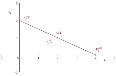
Example 2.4.6. If D consists of the points (0,2),(0,1),(1,0),(2,0) the Newton diagram is formed by the two vertices, Γ(0)1 = (0,1),Γ(0)2 = (1,0) and the edge connecting them Γ(1)1 .
2.4.3
Nonelementary Singular Points
We consider now the system
˙
xi =ϕi(x1, x2), ϕi(0,0) = 0, i= 1,2, (2.4.15)
whereϕiare real analytic and the origin is an isolated nonelementary singular
point. The vector field defined by (2.4.15) can be written as
X(x1, x2) = X
i=1,2 X
Q
fiQ (x1, x2)Qxi ∂ ∂xi
, (2.4.16)
where ϕi(x1, x2) = xifi(x1, x2) and
fi(x1, x2) = X
Q
fiQ (x1, x2)Q. (2.4.17)
As per Bruno’s method, for each element Γ(jd) of the Newton diagram ˆΓ as-sociated with (2.4.16), there is a corresponding sector Ud
j in the phase space R2(x1,x2), so that together they form a full neighbourhood of the origin (here
the boundaries of the sectors are not necessarily integral curves). In each
Ud
(quasihomogeneous blow-ups) which reduces the problem to the study of elementary singularities of the transformed system. This allows one to deter-mine the behaviour of the orbits in each sector. After that the results in each sector are glued together to obtain the overall phase portrait of the system near the origin. We distinguish between two cases: that of a vertex and that of an edge.
The Case of a Vertex. We define aunit vectorR∈R2to be a vector whose
coordinates are coprime integers. Let Q = Γ(0)j be a vertex of ˆΓ. Consider the unit vectors Rj−1 = (r1,j−1, r2,j−1) and Rj = (r1,j, r2,j) directional to
Γ(1)j−1 and Γ(1)j respectively, assuming that r2,j−1 >0 andr2,j >0, so that the
vectors are determined uniquely. Set R∗ = −Rj−1 and R∗ = Rj. If Q is a
boundary point of ˆΓ, we set R∗ = (1,0) if Q is the right boundary point of
ˆ
Γ, denoted as Q∗, and we set R∗ = (0,1) if Q is the left boundary point of
ˆ
Γ, which we denote as Q∗. Bruno’s method associates to Q a set defined by
Uj(0)(ε) = {(x1, x2)∈R2 :(|x1|,|x2|)R
∗
≤ε,
(|x1|,|x2|)R∗ ≤ε,|x1| ≤ε,|x2| ≤ε},
(2.4.18)
for some ε > 0. Applying the change of time coordinate from the old time
τ to τ1 which satisfies dτ1 = (t, s)Qdτ, the system (2.4.15) transforms into
one of the form (2.4.7). The resulting system satisfies the assumptions of the Principal or the Second Normal Form Theorem. The behaviour of the integral curves of the normal form and the original system coincides in Uj(0)(ε) for ε
sufficiently small. See [7, page 138] for a detailed discussion and justification of these facts.
The Case of an Edge. Let Γ(1)j be an edge of ˆΓ and let R = (r1, r2) , r2 > 0 be a unit directional vector of Γ
(1)
j . The corresponding set in the
phase space is given by
U1
j(ε) ={(t, s)∈R
2 :ε≤(|t|,|s|)R ≤1/ε, |t| ≤ε,|s| ≤ε}. (2.4.19)
Consider the power transformation given by y1 = tk1sk2, y2 = tr1sr2, where
the integers k1, k2 are chosen such that the matrix
A=
k1 k2 r1 r2
(2.4.20)
has the determinant equal to 1. In the matrix form, we can writeX = (t, s),
Q=
q1 q2
FQ=
f1q f2q
.
Then (2.4.15) can be given by
˙
(lnX) = X
Q∈D
FQXQ, (2.4.21)
where XQ = tq1sq2. The power transformation can be expressed now as
Y =XA taking (2.4.21) into
˙
(lnY) = X
Q0∈D0
FQ00YQ 0
,
with Y = (y1, y2), Q0 = (AT)−1Q, D0 = (AT)−1D, and FQ00 = AFQ. After
division by the maximal power of y1 one obtains a new system. Here the y2-axis corresponds to {t=s= 0}in the original coordinates, and therefore
Chapter 3
Polynomial Convexity of the
Open Whitney Umbrella
In this Chapter we prove Theorem 1.1.1 (see Section 1.1). The approach uses the method introduced in [36].
3.1
Reduction to a Dynamical System
We first review how the problem of local polynomial convexity near a Whit-ney umbrella can be reduced to the computation of the phase portrait of a certain dynamical system, a method that was introduced in [36]. In fact, the procedure works without modifications for a somewhat more general type of isolated singularities.
3.1.1
The characteristic foliation
Let τ : R2 → R4 ∼=
C2, τ(0) = 0, be a homeomorphism onto its image,
smooth except at the origin, and such thatS =τ(R2) is a totally real surface
in C2 with an isolated singular point at the origin. Suppose S is embedded
in a real hypersurfaceM inC2. We define a field of lines determined at every
p∈S\ {0}by
Lp =TpS∩HpM,
whereHpM =TpM∩J TpM is the complex tangent space ofM atpand J is
curves corresponding to this field is called the characteristic foliation of S
(with respect to M).
Let us also suppose that M is defined as the zero locus of a function
ρ:C2 →
R, smooth and strictly plurisubharmonic near the origin,
M =M(ρ) ={(z, w)∈C2 :ρ(z, w) = 0}, ∇ρ|
M\{0} 6= 0,
and let
Ω(ρ) ={(z, w)∈C2 :ρ(z, w)<0}.
The essential hull Kess of a compact set K ⊂ C2 is defined by Kess =
ˆ
K\K, and itstrace Ktr by Ktr =Kess∩K. We note that
Kess⊆Kdtr. (3.1.1)
Indeed, a local Maximum Principle due to Rossi [33, 40] states that if K is a compact set in Cn,E is a compact subset of ˆK and U is an open subset of
Cn that contains E, then for all f ∈ O(U),kfkE =kfk(E∩K)∪∂E, where the
boundary of E is taken with respect to ˆK. Now, by choosing E =Kess and
U =C2, we obtain (3.1.1).
Sinceτ is continuous, the set S =τ(R2) is connected. Let ε >0 be such
that ρ is strictly plurisubharmonic in B(0;ε). By a classical result (see, for example, [19, 40]), the polynomially convex hull ofS∩B(0;ε) agrees with its psh-hull (see Section 2.2). Hence, the polynomial hull of the set S∩B(0;ε) is contained in Ω(ρ)∩B(0;ε). Let X be the connected component of S∩
B(0;ε) containing the origin. ThenX\ {0}is a smooth compact real surface embedded in∂Ω(ρ). The following key proposition is essentially due to Duval [11] (see also J¨oricke [21]).
Proposition 3.1.1. Xtrcannot intersect a leaf of the characteristic foliation at a totally real point of X without crossing it.
The original proof of Duval can be easily adapted to our situation. It is an application of Oka’s characterization of polynomially convex subsets of
Cn. Oka’s family of algebraic curves can be constructed from the leaves of
the characteristic foliation, and because Ω is strictly pseudoconvex, it suffices to ensure that the family leaves Ω. See [36] for details.
Proposition 3.1.2. Suppose that there exist two rectifiable arcs γ1, γ2 in X such that
(i) γ1∩γ2 ={0};
(ii) γj are smooth at all points except, possibly, at the origin;
(iii) For any compact subset K ⊂ X not contained in γ1 ∪γ2, there exists a leaf γ of the characteristic foliation of S such that K∩γ 6=∅ but K does not meet both sides of γ.
Then, X is polynomially convex.
Proof. It follows from Proposition 3.1.1 that Xtr ⊆γ
1∪γ2 and from (3.1.1)
that Xess ⊆ γ\
1∪γ2. A rectifiable arc is polynomially convex [40,
Corol-lary 3.1.2]. Moreover, by [40, Theorem 3.1.1], if Y is a compact polynomi-ally convex subset of Cn and Γ is a compact connected set of finite length,
then (Y\∪Γ)\(Y ∪Γ) is either empty or it contains a complex purely one-dimensional analytic subvariety of the complementC2\(Y ∪Γ). By takingY
and Γ to be the arcsγ1, γ2, it can be shown by following the same rationale as
in [36, Corollary 2], that the union of the two arcs cannot bound a complex one-dimensional variety. Therefore, γ\1∪γ2 = γ1 ∪γ2 ⊂ X, so Xess ⊂ X.
Since Xb\X ⊆Xess\X =∅, it follows that X is polynomially convex.
Before we proceed to the proof of Theorem 1.1.1 let us present the proof of the corollary stated in Section 1.1, assuming that Theorem 1.1.1 is true. The proof is exactly the same as the one in [36, page 9].
Proof of Corollary 1.1.2. Let φ(0) =p. By Theorem 1.1.1 there exists ε >
0 such that X = φ(Σ)∩B(p, ε) is polynomially convex. For sufficiently small ε we may further assume that φ(Σ)∩∂B(p, ε) is a smooth curve. By the result of J. Anderson, A. Izzo, and J. Wermer [3, Thm. 1.5], if X is a polynomially convex compact subset of Cn, and X0 is a compact subset of X such that X \X0 is a totally real submanifold of Cn, of class C1, then
continuous functions on X can be approximated by polynomials if and only if this can be done on X0. We apply this result to X = φ(Σ)∩B(p, ε) and X0 ={p} ∪(φ(Σ)∩∂B(p, ε)). The set X0, is polynomially convex. Indeed,
if not, we obtain as in the proof of Proposition 3.1.2 that Xb0 \X0 contains
a complex purely 1-dimensional analytic subvariety V of C2\X
example [40], p. 122, continuous functions on X0 can be approximated by
polynomials. From this the corollary follows.
Our next goal is to find a suitable hypersurface containing the open Whit-ney umbrella, such that the properties of Proposition 3.1.2 are satisfied.
3.1.2
The characteristic foliation of the open Whitney
umbrella
We identifyR4(x,u,y,v)withC(2z,w) for computational purposes. IfI2 is the 2×2
identity matrix, we denote by
J =
0 −I2 I2 0
the matrix defining the standard complex structure on C2. Let φ:
C2 →C2
be a local symplectomorphism which, without loss of generality, is assumed to preserve the origin. Let the Jacobian matrix of φ at 0 be
Dφ(0) =
A B
C D
,
whereA, B, C, D are the 2×2 block components given by the partial deriva-tives of φ. Sinceφ is symplectic, we have
AtD−CtB =I2, AtC =CtA, DtB =BtD. (3.1.2)
Let ψ :R4 →R4 be the linear transformation given by the matrix
Ψ =
Dt −Bt Bt Dt
.
Since ΨJ = JΨ, the map ψ is complex linear. We now show that Ψ is invertible. From (3.1.2) we get
D(ψ◦φ)(0) =
I2 0
E G
, E = (eij), eij ∈C, (3.1.3)
where
Since Dψ(0) is symplectic, detDφ(0) = 1, and so detG = det Ψ. We claim that
detG=g11g22−g212>0. (3.1.5)
Indeed, let B = (bjk), and D= (djk). A straightforward computation gives
detG= (b11b22−b12b21)2+ (b11d12−b12d11)2 + (b11d22−b12d21)2
+ (b21d12−b22d11)2 + (b21d22−b22d21)2+ (d11d22−d12d21)2,
which is obviously nonnegative. If detG= 0, then, forj = 1,2, the following hold
(bj2 = 0)⇒(bj1 = 0), (dj2 = 0)⇒(dj1 = 0).
On the other hand, if any two or more of b12, b22, d12, d22do not equal 0, then
the corresponding ratios b11
b12 ,b21
b22 ,d11
d12 ,d21
d22
are equal, e.g., if b12 6= 0, b22 6= 0, d12 6= 0, and d22 6= 0, then
b11 b12
= b21
b22
= d11
d12
= d21
d22
=λ∈R.
It is not difficult to see that all possible combinations lead to Dφ(0) either having two identically zero columns in the verticalB|Dblock, or one column being a λ multiple of another. In both scenarios detDφ(0) = 0, which is a contradiction. It follows then, that detG > 0, which proves that Ψ is nonsingular. Furthermore, (3.1.4) and (3.1.5) imply that g11 >0, g22>0.
Now, let
Σ0 = (ψ◦φ)(Σ),
which by construction is a totally real surface with an isolated singular point at the origin. We consider the following auxiliary hypersurface which contains Σ,
M =M(ρ) ={(z, w)∈C2 :ρ(z, w) :=x2−yv2+9
4u
2−y3+C(xy−3
2uv) = 0}, where C >0. A direct computation shows that for any C >0, the gradient
∇ρ does not vanish in some punctured neighbourhood of the origin. Now, put
M0 = (ψ◦φ)(M) = M0(ρ0), ρ0 :=ρ◦(ψ◦φ)−1.
(ψ◦ϕ)(Σ) is. We next show that, for someC > 0,M0 is strictly pseudoconvex near the origin. Let (x0, u0, y0, v0) be the coordinates in the target space of
ψ◦φ and let
(D(ψ◦φ)(0))−1 =
I2 0 E0 G0
, E0 = (e0ij), G0 = (g0ij), eij, gij ∈C.
The formal Taylor expansion of (ψ◦φ)−1 is given by
(ψ ◦φ)−1(x0, u0, y0, v0) =
x0+σ1, u0+σ2, e011x0+e120 u0+g011y0 +g012v0+σ3,
e021x0+e022u0+g012y0+g022v0+σ4
,
where
σi = X
j+k+l+m≥2
hijklmx0ju0ky0lv0m, hijklm∈C, i∈ {1,2,3,4}.
Then,
ρ0(x0, u0, y0, v0) = (x0 +σ1)2
−(e011x0+e012u0+g011y0 +g012v0+σ3)
·(e021x0+e022u0+g120 y0+g022v0 +σ4)2
+9 4(u
0
+σ2)2−(e011x0 +e012u0+g110 y0+g120 v0+σ3)3 +C(x0+σ1)(e011x0+e012u0 +g011y0+g120 v0+σ3)
− 3C
2 (u
0
+σ2)(e021x0+e022u0+g120 y0+g220 v0+σ4).
A direct computation gives the Levi form ofρ0,
Lρ0 =
2 + 2Ce011 Ce012− 3
2Ce 0 21+ 5i 2Cg 0 12
Ce012− 3
2Ce 0 21− 5i 2Cg 0 12 9
2−3Ce
0 22 .
origin, hence M0 is strictly pseudoconvex in some punctured neighbourhood of the origin. Note that the constant C depends on the symplectomorphism
φ.
We will show that S = Σ0 and M = M0(ρ0) satisfy the conditions of Proposition 4.2.1. For this, in Section 3.2, we compute the dynamical system describing the characteristic foliation of Σ0, and in Section 3.3 we describe the method of reduction to the principal part of a vector field due to Brunella and Miari [6]. We use this in Section 3.4 to determine the phase portrait of the characteristic foliation.
3.2
Calculation of the System
In this section we compute the relevant low order terms of the pullback to the parameterizing plane R2(t,s) of the dynamic system that determines the characteristic foliation of Σ0. We introduce the following notation for the components of the gradient of ρ0,
∇ρ0 = (Rx(t, s), Ru(t, s), Ry(t, s), Rv(t, s)),
and we also set
σxi = ∂σ
i ∂x0, σ
i u =
∂σi ∂u0, σ
i y =
∂σi ∂y0, σ
i v =
∂σi
∂v0, i∈ {1,2,3,4}.
A straightforward computation gives the Jacobian matrix of (ψ◦φ)−1 at the
origin,
D(ψ ◦φ)−1(0) =
I2 0 E0 G0
=
I2 0
−G−1E G−1
. (3.2.1)
The characteristic foliation of Σ0 is determined at every p∈Σ0 \ {0} by
LpΣ0 =TpΣ0 ∩HpM0, HpM0 =TpM0∩J(TpM0).
It follows that
We thus obtain a smooth vector field X ∈TΣ0, given by
X =α∂f ∂t +β
∂f
∂s, (3.2.2)
where f :R2 →R4 is defined as
f =ψ◦φ◦π,
and α, β are smooth functions on R2, satisfying Xp=f(t,s) ∈ Lp=f(t,s)Σ0, for p6= 0. Consequently, we can choose
α(t, s) = hJ∂f ∂s,∇ρ
0i
, β(t, s) =−hJ∂f ∂t,∇ρ
0i
. (3.2.3)
We conclude that the characteristic foliation of Σ0 is defined by the following system of ODE’s
(
˙
t =α(t, s) ˙
s =β(t, s). (3.2.4)
Writing
f(t, s) = (f1(t, s), f2(t, s), f3(t, s), f4(t, s)),
and using (3.1.3) and (1.1.1), we can express eachfi as a formal power series
in (t, s):
f1(t, s) =ts+f021 s 2+f1
12ts 2 +f1
21t
2s+f1 03s
3+ X
j+k≥4
fjk1 tjsk,
f2(t, s) =
2 3t
3+f2 02s
2+f2 12ts
2+f
21t2s+f03s3+ X
j+k≥4
fjk2 tjsk,
f3(t, s) =g12s+g11t2+e11ts+f023s
2+ 2e12
3 t
3+f3 12ts
2
+f213 t2s+f033 s3+ X
j+k≥4
fjk3 tjsk,
f4(t, s) =g22s+g12t2+e21ts+f024s
2+ 2e22
3 t
3+f4 12ts
2
+f214 t2s+f034 s3+ X
j+k≥4
fjk4 tjsk,
From the above identities, putting Xt= ∂f
∂t, Xs= ∂f
∂s, we get
Xt =
s+ 2f211 ts+f121s2
2t2+ 2f2
21ts+f122s2
2g11t+e11s+ 2e12t2+ 2f213 ts+f123 s2
2g12t+e21s+ 2e22t2+ 2f214 ts+f124 s2
+o(|(t, s)|2), (3.2.6)
and
Xs=
t+ 2f021 s+f211 t2+ 2f121 ts+ 3f031s2
2f2
02s+f212t2+ 2f122 ts+ 3f032s2
g12+e11t+ 2f023 s+f213 t2+ 2f123 ts+ 3f033 s2
g22+e21t+ 2f024 s+f214 t2+ 2f124 ts+ 3f034 s2
+o(|(t, s)|2). (3.2.7)
It follows from (3.2.3) that
α(t, s) =−(Xs)3Rx−(Xs)4Ru+ (Xs)1Ry+ (Xs)2Rv = X
j,k≥0
αjktjsk,
β(t, s) = (Xt)3Rx+ (Xt)4Ru−(Xt)1Ry−(Xt)2Rv = X
j,k≥0
βjktjsk,
(3.2.8)
where (Xt)i,(Xs)i, i = 1, . . . ,4, are the components of Xt, Xs, respectively.
Rx = 2A(x0+σ1)(1 +σ1x)−A(e
0
11+σx3)(e
0
21x
0
+e022u0+g120 y0+g220 v0+σ4)2
−2A(e021+σx4)(e021x0+e022u0+g120 y0+g220 v0+σ4)
·(e011x0+e012u0 +g011y0+g120 v0+σ3)
+9 2B(u
0
+σ2)σx2−3B(e011+σx3)(e011x0+e012u0 +g011y0+g120 v0+σ3)2,
+C(1 +σx1)(e011x0 +e012u0+g110 y0+g120 v0 +σ3) +C(x0+σ1)(e011+σx3)
−3
2Cσ
2 x(e
0
21x
0
+e022u0 +g012y0+g022v0+σ4)
−3
2C(u
0
+σ2)(e021+σx4),
Ru = 2A(x0+σ1)σu1 −A(e
0
12+σ 3 u)(e
0
21x
0
+e022u0 +g012y0+g022v0+σ4)2
−2A(e022+σ4u)(e021x0+e022u0 +g012y0+g220 v0+σ4)
·(e011x0+e012u0 +g011y0 +g012v0+σ3)
+9 2B(u
0
+σ2)(1 +σu2)−3B(e012+σu3)(e011x0+e012u0+g110 y0+g120 v0+σ3)2 +Cσu1(e011x0+e012u0+g110 y0+g120 v0+σ3)
+C(x0+σ1)(e012+σu3)
−3
2C(1 +σ
2 u)(e
0
21x
0
+e022u0+g120 y0+g220 v0+σ4)
−3
2C(u
0