1
What’s in a Smile? Initial Analyses of Dynamic Changes
in Facial Shape and Appearance
DJJ Farnell1†, J Galloway1, A Zhurov1, S Richmond1, D. Marshall2, PL Rosin2,
K Al-Meyah2, P Pirttiniemi3,4, and Raija Lähdesmäki3,4
1School of Dentistry, Cardiff University, Heath Park, Cardiff CF14 4XY, UK
2School of Computer Science and Informatics, Cardiff University, CF24 3AA, Cardiff, UK.
3Research Unit of Oral Health Sciences, Faculty of Medicine, University of Oulu, Oulu,
Finland
4Medical Research Center Oulu (MRC Oulu), Oulu University Hospital, Oulu, Finland
[email protected] (†corresponding author)
[email protected] [email protected] [email protected] [email protected]
2
Abstract
Single-level Principal Components Analysis (PCA) and multi-level PCA (mPCA) methods are applied here to a set of (2D frontal) facial images from a group of 80 Finnish subjects (34 male; 46 female) with two different facial expressions (smiling and neutral) per subject. Inspection of eigenvalues gives insight into the importance of different factors affecting shapes, including: biological sex, facial expression (neutral versus smiling), and all other variations. Biological sex and facial expression are shown to be reflected in those components at appropriate levels of the mPCA model. Dynamic 3D shape data for all phases of a smile made up a second dataset sampled from 60 adult British subjects (31 male; 29 female). Modes of variation reflected the act of smiling at the correct level of the mPCA model. Seven phases of the dynamic smiles are identified: rest pre-smile, onset 1 (acceleration), onset 2 (deceleration), apex, offset 1 (acceleration), offset 2 (deceleration), and rest post-smile. A clear cycle is observed in standardized scores at an appropriate level for mPCA and in single-level PCA. mPCA can be used to study static shapes and images, as well as dynamic changes in shape. It gave us much insight into the question “what’s in a smile?”
Keywords: multilevel principal components analysis; shape and image texture; facial expression
3
Introduction
Human faces are central to our identity and they are important in expressing emotion. The act of smiling is important in this context and the exploration of facial changes and dynamics during the act of smiling [1,2] is an ongoing topic of investigation in fields of research in orthodontics and prosthodontics, both of which aim to improve the function and appearance of dentition. Aesthetics (e.g., of smiles [3]) are therefore an important aspect of these fields. Much research into the “science of a smile” also focuses on the effects of aging and biological sex on the shape and appearance [4-5] and also the dynamics [6-8] of smiling. Recent investigations have been greatly enhanced by the use of three-dimensional (3D) imaging techniques [9-13] that allow both static and dynamic imaging of the face. Clinically, this research has led to improved understanding of orthognathic surgery [9], malocclusion [10], associations between facial morphology and cardiometabolic risk [11], lip shape during speech [12], facial asymmetry [13], and sleep apnea [14] (to name but a few examples). Clearly also, facial simulation is of much interest for human-computer interfaces (see, e.g., Refs. [15,16]). The role of genetic factors on facial shape has also been the subject of much recent attention [17-20] and many factors (sex, age, and genetic factors) across a set of subjects can affect the shape and dynamics of facial and / or mouth shape.
4
effects was observed. Finally, principal component “scores” also showed strong clustering, which were again at the correct levels of the mPCA model.
Another method that allows us to investigate the effects of covariates on facial shape to be modeled is called bootstrapped response-based imputation modeling (BRIM) [19-20]. The effects of covariates such as sex and genomic ancestry on facial shape were summarized in Ref. [19] as response-based imputed predictor (RIP) variables and the independent effects of particular alleles on facial features were uncovered. Indeed, the importance of modeling the effects of covariates in images is also becoming increasingly recognized, e.g., such as in variational auto-encoders (see, e.g., Refs. [37-39]) in which the effects of covariates are modeled as latent variables sandwiched between encoding (convolution) and decoding (deconvolution) layers. However, the topic of variational auto-encoders lies beyond the scope of this article. Linear discriminant functions have also been used previously (see, e.g., Refs. [40.41]) to explore groupings in the subject population for image data.
Figure 1. Flowchart illustrating the multilevel model of facial shape for dataset 1
The work presented here is also an expansion of Ref. [25] that extended the mPCA approach from shape data also to include image data, where a set of (frontal) facial images from a group of 80 Finnish subjects (34 male; 46 female) each for two different facial expressions (smiling and neutral) were considered. A three-level model illustrated by Figure 1 was constructed that contains biological sex, facial expression, and “between-subject variation” at different levels of the model and we use this model again here for this dataset. However, we also compare results of mPCA to those results of single-level PCA, which was not carried out in Ref. [25]. Furthermore, the dynamic aspects of a smile are considered here in a new (time series) dataset of 3D mouth shape captured during all phases of a smile, which was also not considered in Ref. [25]. We present here firstly the subject characteristics and details of image capture and
Level 1
• Variation due to biological sex
Level 2
• Between-subject variation: all other
variation not due to sex or facial expression
Level 3
• Within-subject variation: facial
5
6
Materials and Methods
Image Capture, Preprocessing, and Subject Characteristics
Figure 2. Illustration of the 21 landmark points for dataset 1 ((1) Glabella (g); (2) Nasion (n); (3) Endocanthion left (enl); (4) Endocanthion right (enr); (5) Exocanthion left (exl); (6) Exocanthion right (exr); (7) Palpebrale superius left (psl); (8) Palpebrale superius right ( psr); (9) Palpebrale inferius left ( pil); (10) Palpebrale in-ferius right (pir); (11) Pronasale (prn); (12) Subnasale (sn); (13) Alare left (all); (14) Alare right (alr); (15) Labiale superius (ls); (16) Crista philtri left (cphl); (17) Crista philtri right (cphr); (18) Labiale inferius (li); (19) Cheilion left (chl); (20) Cheilion right (chr); (21) Pogonion (pg)).
7
points are used here in the analysis of shape. Preprocessing of the shapes included centering, alignment, and adjustment of overall scale only. Preprocessing of image texture [25] also included the definition of a region of interest (ROI) around edges of the face (7339 pixels) and the overall illumination of the grayscale images was standardized.
Dataset 2 consisted of 3D video shape data during all phases of a smile, where 13 points placed (and tracked) along the outer boundary of mouth. Subjects were 60 adult staff and students at Cardiff University (31 male and 29 female). The number of frames in the video was between approximately 100 and 250 frames during all phases of a smile for each subject. In these initial calculations, preprocessing consisted of centering the 3D shapes only. The (normalized) smile amplitude was defined by using the following equation
0 at time chelion right and left the between Distance 2 at time chelion right and left the between Distance Amplitude Smile = × = t t
. (1)
8
Figure 3. Schematic illustration of a time series of smile amplitudes from Eq. (1) for 3D shape data in dataset 2. Including rest phases, seven phases can be identified manually: rest pre-smile; onset acceleration; onset deceleration; apex; offset acceleration; offset deceleration; and, rest post-smile.
Multilevel Principal Components Analysis (mPCA)
ASMs [26-30] are statistical models of shape only and AAMs [31-36] are statistical models of both shape and appearance. The term “image texture” is taken to refer to the pattern of intensities or colors across an image (or image patch) as in AAMs and we adopt this usage here. For ASMs, features may be segmented from an image by firstly forming the shape model over some “training” set of shapes. Single-level principal component analysis (PCA) may be used to define the distributions of points or intensities (and / or color) at given pixel positions, respectively. For single-level PCA of shape, the mean shape vector (averaged over all N subjects) is given by z and a covariance matrix, C, is then found by evaluating
) ( ) ( 1 1 2 2 1 1 2 1 1
, ik ik
N
i
ik ik k
k z z z z
N
C − −
−
=
=
, (2)
where k1 and k2 indicate elements of this covariance matrix. We find the eigenvalues λl and (orthonormal) eigenvectors ul of this matrix. All eigenvalues are non-negative, real numbers because covariance matrices are symmetric and positive semi-definite. For PCA, one ranks all of the eigenvalues λl into descending order and we retain the first l1 components in the model.
Any new shape is then modeled by
= + = 1 1 l l l l au zz . (3)
The coefficients, al, for a fit of the model to a new shape vector, z, are found readily by using a scalar product with respect to the set of orthonormal eigenvectors ul, i.e.,
) (z z u ⋅ −
= l
l
a , (4)
9
al. This process is iterated until convergence and so the final segmentation never “strays too far” from a plausible solution with respect to the underlying shape model. In this article, we are concerned only with the modeling of shape and appearance and we do not carry out the “active” image searches. However, the methods presented here could be extended to such image searches via ASMs or AAMs, although this is not the primary focus of this article.
Multilevel PCA (mPCA) allows us to isolate the effects of various influences on shape or image texture at different levels of the model. For the case of the act of “smiling,” this allows us to adjust for each subjects’ individual shape or appearance (and biological sex also for dataset 1) in order can get a clearer picture of these general changes due to a primary factor (here, facial expression due to smiling). This is illustrated schematically in Figure 1 for dataset 1. Multiple levels are used in mPCA to model the data and covariance matrices are formed at each level. For the model for dataset 1 illustrated by Figure 1, the covariance matrix at level 3 is formed with respect to the two expressions (neutral smiling) for each subject and then these covariance matrices are averaged over all 80 subjects. By contrast, the covariance matrix at level 2 is formed with respect to shapes or image texture averaged over the 2 expressions for each of the 80 subjects. Covariance matrices are formed for males and females separately and then they are averaged over 2 sexes to find the final covariance matrix at level 2 of this model. Finally, the covariance matrix at level 2 is formed with respect to shapes or image texture sex only, i.e., averaged over all subjects and expressions for the two sex groups separately. The number of shapes or images equals 2 at this level of the model and so the rank of this matrix is 1. Clearly, any restriction on the rank of the covariance matrix is a limitation of the mPCA model, although other multilevel methods (such as multilevel Bayesian approaches) ought not to be as strongly constrained as mPCA. An exploration of these topics will form the contents of future research. A three-level mPCA model was also used in this initial exploration for dataset 2: level 1, “between subject” due to natural face shape not attributed to smiling; level 2, “between smile phases” variation due to differences between seven different phases of a smile; level 3, “within smile phases” variation due to residual differences within the different phases of a smile.
mPCA then uses PCA with respect to these covariance matrices at each of the three levels separately. The lth eigenvalue at level 1 is denoted by 1
l
λ with associated eigenvector 1 l
u, whereas
the lth eigenvalue at level 2 is denoted by 2 l
λ with associated eigenvector is denoted by 2 l
u , and
10
separately, and then we retain the first l1, l2 … eigenvectors of largest magnitude for all of the
levels, respectively. Any new shape is modeled by
= = = + + += 1 2 3
1 3 3 1 2 2 1 1 1 l
l l l l
l l l l
l l l
a a
au u u
z
z , (5)
where z is the “grand mean.” The coefficients { 1},{ 2},
l l a
a (also referred to here as
“component scores”) are determined for any new shape, z, by using a global optimization procedure in MATLAB R2017 with respect to the cost function
2 1 3 3 1 2 2 1 1 1 1 2 1 ) ( )
(
1
2
3
= = = = = − − − − = − = Δ ll l lk l l lk l l l lk l k k k k k
k z z z au a u au
z model . (6)
(Note again that zk is the kth element of the shape vector z, and ulk1 indicates the kth element of
the lth eigenvector at level 1 (etc.)) Another method of obtaining a solution is to iterate the
following equations directly,
α α α κ l l l a a a ∂ Δ ∂ −
← (7)
(where α = 1, 2, 3, here and for all values l appropriately) for our three-level models from some “starting point” (often taken to be the average shape, i.e., all coefficients are zero) until convergence. (An appropriate choice of κ is found to be κ = 0.01.) It is straightforward to see that
= = = − − − − − = ∂ Δ ∂ k l m mk m l m mk m l m mk m k k lk l u a u a u a z z ua 2 ( )
3 2 1 1 3 3 1 2 2 1 1 1 α
α . (8)
Note that this approach finds identical solutions to that provided by MATLAB. Finally, standardized coefficients may be found by dividing the {al} coefficients by the square root of
the corresponding eigenvalue λl for single-level PCA and by dividing the {a1m} coefficients by
the square root of the corresponding eigenvalue 1
m
11 3 Results
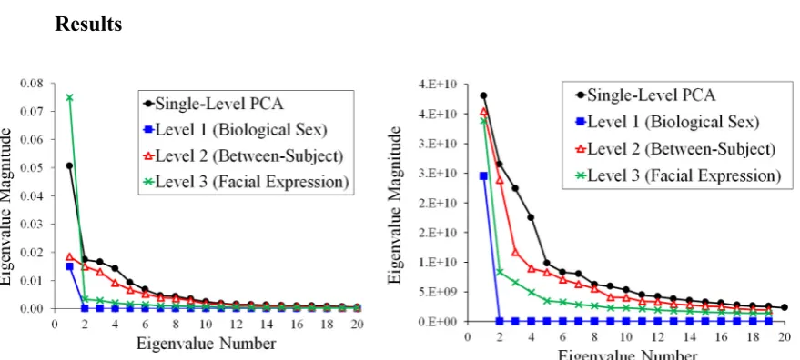
Figure 4. Eigenvalues for dataset 1 from single-level PCA and from mPCA level 1 (biological sex), level 2 (between-subject variation), and level 3 (within-subject variation: facial expression). (Left) shape data; (Right) image texture data. (All shapes have been scaled so that the average point-to-centroid distance equals 1.)
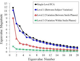
Eigenvalues for both shape and also image texture via mPCA are shown in Figure 4 for dataset 1. The results for mPCA demonstrated a single non-zero eigenvalue for the level 1 (biological sex). A single large eigenvalue for the level 3 (facial expression) for mPCA occurs for shape and also for image texture, although many non-zero (albeit of much smaller magnitude) eigenvalues occur for image texture. Level 2 (between-subjects variation) via mPCA tends to have the largest number of non-zero eigenvalues for both shape and image texture. The first two eigenvalues are (relatively) large at level 2, mPCA for image texture. mPCA results suggest that biological sex seems be the least important for this group of subjects for both shape and texture, although caution needs to be exercised as the rank of the matrix is 1 at this level for both shape and texture. Results for the eigenvalues from single-level PCA are of comparable magnitude to those results of mPCA, as one would expect, and they follow a very similar pattern. Inspection of these results for the eigenvalues tell us broadly that facial expression and natural facial shape (not dependent on sex or expression) are strong influences on facial shapes in the dataset. Biological sex was found to be a weaker effect comparatively, especially for shape, although again caution needs to be exercised in interpreting eigenvalues at this level for mPCA.
12
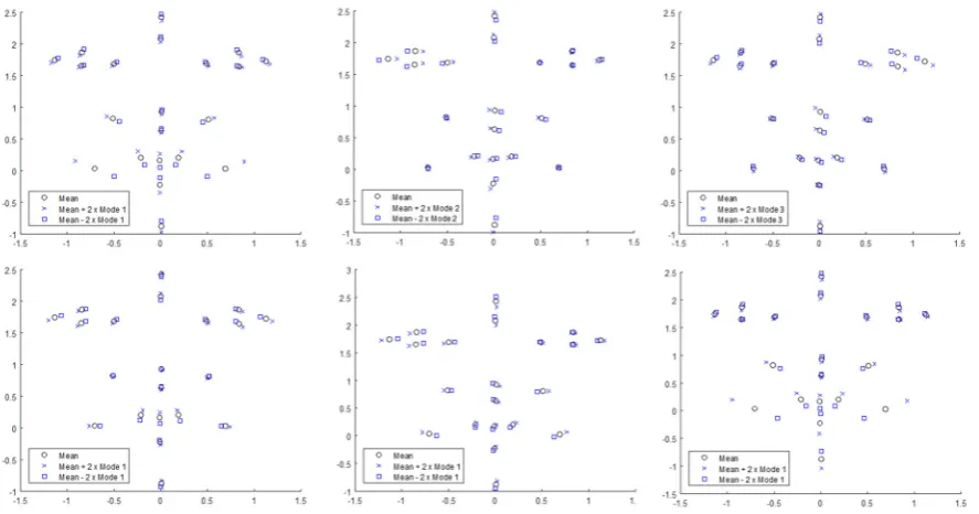
Figure 5. Modes of variation for shape for dataset 1 for the first three modes from single-level PCA in the upper set of images: top left = mode 1; top middle = mode 2; top right = mode 3. The first modes from levels 1 to 3 mPCA in the bottom set of images: bottom left = mode 1, level 1 (biological sex); bottom middle = mode 1, level 2 (between subjects); bottom right = mode 1, level 3 (facial expression).
13
mPCA should focus more clearly on individual influences because they are modeled at different levels of the mPCA model. The first mode at level 2 (between-subject variation) for mPCA in Figure 5 (middle row) corresponds to changes in the relative thinness / width of the face (presumably) that can occur irrespective of sex.
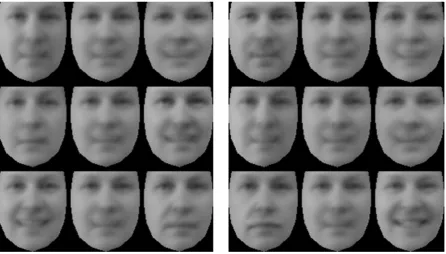
Figure 6. Modes of variation for image texture for dataset 1 for the first three modes (top = mode 1; middle = mode 2; bottom = mode 3) from single-level PCA in the left-hand set of images, and the first modes from levels 1 to 3 (top = level 1; middle = level 2; bottom = level 3) from mPCA in the right-hand set of images. (Note that for each set of three images: left image = mean – SD; middle image = mean; right image = mean + SD.)
14
to interpret, although arguably less so than for the first mode at each level from mPCA. For example, mode 1 possibly corresponds to residual changes in illumination and / or also to slight changes to the nose and prominence of the cheeks, which might be associated with biological sex [43,44]. Modes 2 and 3 correspond clearly to changes due to the act of smiling.
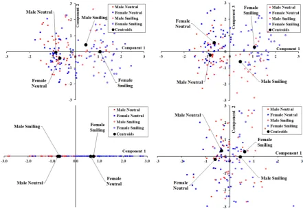
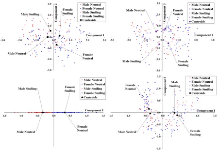
Figure 7. Standardized component scores with respect to shape for dataset 1: (top left) Components 1 and 2 for single-level PCA; (top right) Components 1 and 3 for single-level PCA; (bottom left) Component 1 for level 1 (biological sex) for mPCA; (bottom right) Components 1 and 2 for level 3 (facial expression) for mPCA.
15
mPCA. The centroids in Figure 7 at level 3 (facial expression) for mPCA are strongly separated by facial expression (neutral, smiling), although not by biological sex. Strong clustering by facial expression (alone) is therefore observed at level 3 (facial expression) for mPCA, also as required. Strong clustering by facial expression or biological sex is not seen at level 2 (between-subject variation) mPCA (not shown here), i.e., all centroids by biological sex and facial expression are congruent on the origin.
Figure 8. Standardized component scores with respect to image texture for dataset 1: (top left) Components 1 and 2 for single-level PCA; (top right) Components 1 and 3 for single-level PCA; (bottom left) Component 1 for level 1 (biological sex) for mPCA; (bottom right) Components 1 and 2 for level 3 (facial expression) for mPCA.
16
Figure 9. Eigenvalues for dataset 2 (shape data only) from single-level PCA and from mPCA level 1 (between-subject variation), level 2 (variation between smile phases), and level 3 (variation within smile phases).
17
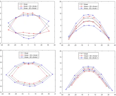
Figure 10. Modes of variation for dataset 2 from mPCA: (top left) level 1 (between-subjects variation), mode 1, coronal plane; (top right); level 1 (between-subjects variation), mode 1, transverse plane; (bottom left) level 2 (variation between smile phases), mode 1, coronal plane; (bottom right) level 2 (variation between smile phases), mode 1, transverse plane.
18
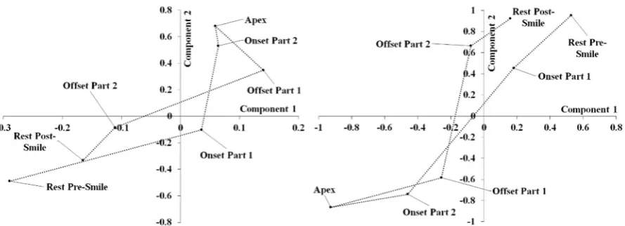
Figure 11. Centroids over smile phases for standardized component scores with respect to shape for dataset 2: (left) Components 1 and 2 for single-level PCA; (right) Components 1 and 2 at level 2 (variation between smile phases) for mPCA.
19
Conclusions
We have shown in this article that mPCA provides a viable method of accounting for groupings in our population subject set and / or for adjusting for potential confounding covariates. For example, natural face or lip shape was represented at one level of the mPCA model and shapes changes due to the act of smiling at another level (or levels) of the model. By capturing these different sources of variation we represented at different levels of the model, we are able to isolate those changes in expression due to smiling that are consistent over the entire populate much more effectively than single-level PCA. All results were found to agree with results of single-level PCA, although mPCA results were (arguably) easier to interpret than those results of single-level PCA.
For the first dataset considered here that contained two “expressions” per subject (neutral or smiling), both obvious effects (widening of the mouth, corners of mouth raised slightly, exposure of teeth, and increased prominence of cheeks) and subtle effects (narrowing of the eyes and a slight widening at bottom of nose during smile) were detected in major modes of variation for the facial expression level of the mPCA model. Inspection of eigenvalues suggested that facial expression and “between-subject” effects were strong influences on shape and image texture, although biological sex was a weaker effect especially for shape. Indeed, another study [24] has noted that sexual dimorphism was weakest for a Finnish population in comparison to other ethnicities (i.e., English, Welsh, and Croatian). Furthermore, the first major mode for shape showed clearly that males have longer / thinner faces on average than women [43,44] at an appropriate level of the mPCA model. Changes in image texture also clearly corresponded to biological sex, again at an appropriate level of the mPCA model. Model fits gave standardized scores for each principal component / mode of variation that show strong clustering for both shape and texture by biological sex and facial expression also at appropriate levels of the model. mPCA correctly decomposes sources of variation due to biological sex and facial expression (etc.). These results are an excellent initial test of the usefulness of mPCA in terms of modeling either shape or image texture.
20
includes rests pre and post smiling, standardized component scores from both mPCA (at the appropriate level of the model) and single-level PCA demonstrated clear evidence of a cycle containing seven phases of a smile: rest pre-smile, onset 1 (acceleration), onset 2 (deceleration), apex, offset 1 (acceleration), offset 2 (deceleration), and rest post-smile. This is strong evidence that seven phases of a smile do indeed exist and it is another excellent test of the mPCA method, now also for dynamic 3D shape data. Furthermore, by considering two separate datasets, we have shown that mPCA has thereby given us much insight into the question: “what’s in a smile?”
Future research will focus on modeling the effects of ethnicity, gender, age, genetic information, or diseases (e.g., effects perhaps previously hidden in the “final 5% of variation”) on facial shape or appearance. The present study has not considered the effects of “outliers” in the shape or image data. Clearly, the effects of outliers (either as isolated points, subjects or indeed even entire groups of subjects) might strongly affect mean averages used to estimate centroids of groups and also covariance matrices at the various levels of the model. The simplest method of addressing this problem is to use robust centroid and covariance matrix estimation [45-47] and then to carry out PCA as normal at each level. Note that robust covariance matrix estimation is included in MATLAB (2017a) and so this may be implemented easily, although a sample size of at least twice the length of the feature vector z is required. Furthermore, the mPCA method uses averages of covariance matrices (e.g., over all subjects in the population or over specific subgroups) and robust averaging of these matrices might also be beneficial. Clearly also, we can use other forms of robust PCA [48-50] and M-estimators [51,53] might also to deal with the problem of outliers. Finally, future research will attempt to extend existing single-level probabilistic methods of modeling shape and / or appearance (e.g., mixtures models [29,53] and extensions of Bayesian methods used in ASMs or AAMs [54-55]) to multilevel formulations. The use of schematics such as Figure 1 will hopefully prove just as useful in visualizing these models as they have for mPCA.
21
component “scores,” especially for small numbers of mark-up points, although this did not seem to be a problem here. However, it might be that certain covariates affect facial or mouth shape in ways that are, in fact, inherently non-orthogonal. mPCA method provides a way of addressing this issue, whereas we would strongly expect single-level PCA to mix effects between different covariates in the principal components in such cases.
22
Author Contributions. Conceptualization: S.R., D.M., P.L.R., R.L., P.P.; Methodology: D.J.J.F., J.G.; Software: D.J.J.F., A.Z.; Investigation: R.L., P.P., K.A.-M., D.J.J.F; Writing, Original Draft Preparation: D.J.J.F.; Writing, Review & Editing: All Authors. Supervision: D.M., P.L.R.; Funding Acquisition: R.L.
Funding: NFBC1966 received financial support from University of Oulu Grant no. 24000692, Oulu University Hospital Grant no. 24301140, ERDF European Regional Development Fund Grant no. 539/2010 A31592.
Acknowledgments: We thank all cohort members and researchers who participated in the “46 years” study. We also wish acknowledge the work of the NFBC project center.
23 References
1. Sarver, D.M.; Ackerman, M.B. Dynamic smile visualization and quantification: part 1. Evolution of the concept and dynamic records for smile capture. Am. J. Orthod. Dentofacial Orthop. 2003, 124, 4–12. DOI: 10.1016/S0889-5406(03)00306-8
2. Sarver, D.M.; Ackerman, M.B. Dynamic smile visualization and quantification: Part 2. Smile analysis and treatment strategies. Am. J. Orthod. Dentofacial Orthop. 2003, 124, 116–27. DOI: 10.1016/S0889-5406(03)00307-X
3. Dong, J.K.; Jin, T.H.; Cho, H.W.; Oh, S.C. The esthetics of the smile: a review of some recent studies. Int. J. Prosthodont. 1999, 12, 9–19.
4. Otta, E. Sex differences over age groups in self–posed smiling in photographs. Psychol. Rep. 1998, 83, 907–13. DOI: 10.2466/pr0.1998.83.3.907
5. Drummond, S.; Capelli Jr, J. Incisor display during speech and smile: Age and gender correlations. Angle Orthod. 2015, 86, 631–7. DOI: 10.2319/042515-284.1
6. Chetan, P.; Tandon, P.; Singh, G.K.; Nagar, A.; Prasad, V.; Chugh, V.K. Dynamics of a smile in different age groups. Angle Orthod. 2012, 83, 90–6. DOI: 10.2319/040112-268.1
7. Dibeklioğlu, H.; Gevers, T.; Salah, A.A.; Valenti, R. A smile can reveal your age: Enabling facial dynamics in age estimation. In Proceedings of the 20th ACM
International Conference on Multimedia 2012 (pp. 209–218). DOI:
10.1145/2393347.2393382
8. Dibeklioğlu, H.; Alnajar, F.; Salah, A.A.; Gevers T. Combining facial dynamics with appearance for age estimation. IEEE Trans. Image Process.2015, 24, 1928–43. DOI: 10.1109/TIP.2015.2412377
9. Kau, C.H.; Cronin, A.; Durning, P.; Zhurov, A.I.; Sandham, A.; Richmond, S. A new method for the 3D measurement of postoperative swelling following orthognathic surgery. Orthod. Craniofac. Res. 2006, 9, 31–7. DOI: 10.1111/j.1601-6343.2006.00341.x
10. Krneta, B.; Primožič, J.; Zhurov, A.; Richmond, S.; Ovsenik, M. Three-dimensional evaluation of facial morphology in children aged 5–6 years with a Class III malocclusion. Eur. J. Orthod.2012, 36, 133–9. DOI: 10.1093/ejo/cjs018
24
and cardiometabolic risk factors in adolescence. BMJ Open. 2013, 3, e002910. DOI: 10.1136/bmjopen-2013-002910
12. Popat, H.; Zhurov, A.I.; Toma, A.M.; Richmond, S.; Marshall, D.; Rosin, P.L. Statistical modeling of lip movement in the clinical context. Orthod. Craniofac. Res. 2012, 15, 92–102. DOI: 10.1111/j.1601-6343.2011.01539.x
13. Alqattan, M.; Djordjevic, J.; Zhurov, A.I.; Richmond, S. Comparison between landmark and surface–based three–dimensional analyses of facial asymmetry in adults.
Eur. J. Orthod.2013, 37, 1–2. DOI: 10.1093/ejo/cjt075
14. Al Ali, A.; Richmond, S.; Popat, H.; Playle, R.; Pickles, T.; Zhurov, A. I.; Marshall, D., Rosin, P. L.; Henderson, J.; Bonuck, K. The influence of snoring, mouth breathing and apnoea on facial morphology in late childhood: a three–dimensional study. BMJ Open. 2015, 5, e009027. DOI: 10.1136/bmjopen-2015-009027
15. Vandeventer, J. 4D (3D Dynamic) statistical models of conversational expressions and the synthesis of highly–realistic 4D facial expression sequences. PhD thesis, Cardiff University, 2015.
16. Vandeventer, J.; Graser, L.; Rychlowska, M.; Rosin, P.L.; Marshall, D. Towards 4d coupled models of conversational facial expression interactions. In Proceedings of the British Machine Vision Conference. 2015, pp 142–1. DOI: 10.5244/C.29.142
17. Paternoster, L.; Zhurov, A.I.; Toma, A.M.; Kemp, J. P.; St. Pourcain, B. ; Timpson, N.J.; McMahon, G.; McArdle, W.; Ring, S.M.; Davey Smith, G.; Richmond, S.; Evans, D.M. Genome–wide Association Study of Three–Dimensional Facial Morphology Identifies a Variant in PAX3 Associated with Nasion Position. Am. J. Hum. Genet. 2012, 90, 478–485. DOI: 10.1016/j.ajhg.2011.12.021
18. Fatemifar, G; Hoggart, C.J.; Paternoster, L.; Kemp, J.P.; Prokopenko. I.; Horikoshi, M.; Wright, V.J.; Tobias, J.H.; Richmond, S.; Zhurov, A.I.; Toma, A.M. Genome– wide association study of primary tooth eruption identifies pleiotropic loci associated with height and craniofacial distances. Hum. Mol. Gen. 2013, 22, 3807–17. DOI: 10.1093/hmg/ddt231
19. Claes, P.; Hill, H.; Shriver, M.D. Toward DNA–based facial composites: preliminary results and validation. Forensic. Sci. Int. Genet. 2014, 13, 208–16. DOI: 10.1016/j.fsigen.2014.08.008
25
Based Twin Study. PLoS ONE. 2016, 11, e0162250. DOI: 10.1371/journal.pone.0162250
21. Lecron F, Boisvert J, Benjelloun M, Labelle H, Mahmoudi S. Multilevel statistical shape models: a new framework for modeling hierarchical structures. Proceedings of 2012 9th IEEE International Symposium on Biomedical Imaging (ISBI). 2012, pp. 1284–1287. DOI: 10.1109/ISBI.2012.6235797
22. Farnell, D.J.J.; Popat, H.; Richmond, S. Multilevel principal component analysis (mPCA) in shape analysis: A feasibility study in medical and dental imaging. Comput. Methods Programs Biomed. 2016, 129, 149–59. DOI: 10.1016/j.cmpb.2016.01.005 23. Farnell, D.J.J.; Galloway, J.; Zhurov, A.; Richmond, S.; Perttiniemi, P.; Katic, V. Initial
results of multilevel principal components analysis of facial shape. In Annual Conference on Medical Image Understanding and Analysis. 2017, pp. 674–685. Springer, Cham. DOI: 10.1007/978-3-319-60964-5_59
24. Farnell, D.J.J.; Galloway, J.; Zhurov, A.; Richmond, S.; Perttiniemi, P.; Katic, V. An Initial Exploration of Ethnicity, Sex, and Subject Variation on Facial Shape – in preparation.
25. Farnell D.J.J., Galloway J., Zhurov A., Richmond S., Pirttiniemi P., Lähdesmäki R. (2018) What’s in a Smile? Initial Results of Multilevel Principal Components Analysis of Facial Shape and Image Texture. Communications in Computer and Information Science. 2018, 894 (Springer, Cham), 177–188. DOI: 10.1007/978-3-319-95921-4_18 26. Cootes, T.F.; Hill, A.; Taylor, C.J.; Haslam, J. Use of Active Shape Models for Locating Structure in Medical Images. Image Vis. Comput. 1994, 12, 355–365. DOI: 10.1016/0262-8856(94)90060-4
27. Cootes, T.F.; Taylor, C.J.; Cooper, D.H.; Graham, J. Active Shape Models - Their Training and Application. Comput. Vis. Image Und. 1995, 61, 38–59. DOI: /10.1006/cviu.1995.1004
28. Hill, A.; Cootes, T.F.; Taylor, C.J. (1996) Active shape models and the shape approximation problem. Image Vis. Comput. 1996, 12, 601–607. DOI: 10.1016/0262-8856(96)01097-9
29. Cootes, T.F.; Taylor, C.J. A mixture model for representing shape variation. Image Vis. Comput. 1999, 17, 567–573. DOI: 10.1016/S0262-8856(98)00175-9
26
bone mineral density from dental radiographs using statistical shape models. IEEE Trans. Inf. Technol. Biomed. 2007, 11, 601–610. DOI: 10.1109/TITB.2006.888704 31. Edwards GJ, Lanitis A, Taylor CJ, and Cootes T. Statistical Models of Face Images:
Improving Specificity. In British Machine Vision Conference 1996, Edinburgh, UK, 1996. DOI: 10.1016/S0262-8856(97)00069-3
32. Taylor, C.J.; Cootes, T.F.; Lanitis, A.; Edwards, G.; Smyth, P.; Kotcheff, A.C. Model– based interpretation of complex and variable images. Philos. Trans. R. Soc. Lond. Biol. 1997, 352, 1267–74. DOI: 10.1098/rstb.1997.0109
33. Edwards, G.J.; Cootes, T.F.; Taylor, C.J. Face recognition using active appearance models. In: Burkhardt H., Neumann B. (eds) Computer Vision. Lecture Notes in Computer Science. 1998, 1407, 581–595. (Springer, Berlin, Heidelberg.) DOI: 10.1007/BFb0054766
34. Cootes, T.F.; Edwards, G.J.; Taylor, C.J. Active appearance models, IEEE Trans. Pattern Anal. Mach. Intell. 2001, 23, 681–685. DOI: 1 0.1109/34.927467
35. Cootes, T.F.; Taylor, C.J. Anatomical statistical models and their role in feature extraction. Br. J. Radiol. 2004, 77, S133–S139. DOI: 10.1259/bjr/20343922
36. Matthews, I.; Baker, S. Active Appearance Models Revisited. Int. J. Comput. Vis. 2004, 60, 135–164. DOI: 10.1023/B:VISI.0000029666.37597.d3
37. Doersch, C. Tutorial on variational autoencoders. arXiv:1606.05908. 2016.
38. Pu, Y.; Gan, Z.; Henao, R.; Yuan, X.; Li, C.; Stevens, A.; Carin L. Variational autoencoder for deep learning of images, labels and captions. In Advances in neural information processing systems. 2016, pp. 2352–2360.
39. Wetzel, S.J. Unsupervised learning of phase transitions: From principal component analysis to variational autoencoders. Phys. Rev. E. 2017, 96, 022140. DOI: 10.1103/PhysRevE.96.022140
40. Etemad, K.; Chellappa, R. Discriminant analysis for recognition of human face images. J. Opt. Soc. Am. A 1997, 14, 1724–1733. DOI: 10.1364/JOSAA.14.001724
41. Kim, T–K.; Kittler, J. Locally Linear Discriminant Analysis for Multimodally Distributed Classes For Face Recognition with a Single Model Image. IEEE Trans. Pattern Anal. Mach. Intell. 2005, 27, 318–327. DOI: 10.1109/TPAMI.2005.58
27
43. Velemínská, J.; Bigoni, L.; Krajíček, V.; Borský, J.; Šmahelová, D.; Cagáňová, V.; Peterka, M. Surface facial modeling and allometry in relation to sexual dimorphism. HOMO 2012, 63, 81–93. DOI: 10.1016/j.jchb.2012.02.002
44. Toma, A.M.; Zhurov, A.; Playle, R.; Richmond, S. A three–dimensional look for facial differences between males and females in a British–Caucasian sample aged 15 ½ years old. Ortho. Craniofacial Res. 2008, 11, 180–185. DOI: 10.1111/j.1601-6343.2008.00428.x
45. Rousseeuw, P.J.; Driessen, K.V. A fast algorithm for the minimum covariance determinant estimator. Technometrics. 1999, 41, 212–23. DOI: 10.1080/00401706.1999.10485670
46. Maronna, R.; and Zamar, R.H. Robust estimates of location and dispersion for high dimensional datasets.” Technometrics. 2002, 50, 307–317. DOI: 10.1198/004017002188618509
47. Olive, D.J. “A resistant estimator of multivariate location and dispersion.” Comput. Stat. Data An. 2004, 46, 99–10. DOI: 10.1016/S0167-9473(03)00119-1
48. Candès, E.J.; Li, X.; Ma, Y.; Wright, J. Robust principal component analysis? JACM. 2011, 58, 11. DOI: 10.1145/1970392.1970395
49. Wright, J.; Ganesh, A.; Rao, S.; Peng, Y.; Ma, Y. Robust principal component analysis: Exact recovery of corrupted low–rank matrices via convex optimization. In Advances in neural information processing systems 2009, pp. 2080–2088.
50. Hubert, M.; Engelen, S. Robust PCA and classification in biosciences. Bioinformatics. 2004, 20, 1728–1736. DOI: 10.1093/bioinformatics/bth158
51. Andersen, R. Modern Methods for Robust Regression. Quantitative Applications in the Social Sciences. 152. Los Angeles, CA: Sage Publications. 2008. ISBN 978-1-4129-4072-6.
52. Godambe, V. P. Estimating functions. Oxford Statistical Science Series. 7. New York: Clarendon Press. 1991. ISBN 978-0-19-852228-7.
53. Ulukaya, S.; Erdem, C.E. Gaussian mixture model based estimation of the neutral face shape for emotion recognition. Digit. Signal Process. 2014, 32, 11–23. DOI: 10.1016/j.dsp.2014.05.013
28