Stratified Finite Empirical Bernstein Sampling

Stratified Finite Empirical Bernstein

Sampling

Mark Alexander Burgess∗ and Archie C. Chapman Australian National University

College of Engineering and Computer Science Canberra ACT 2600, Australia e-mail:[email protected]

The University of Sydney School of Electrical and Information Engineering Sydney NSW 2006, Australia e-mail:[email protected]

Abstract: We derive a concentration inequality for the uncertainty in stratified random sampling. Minimising this inequality leads to an iterated online method for choosing samples from the strata. The inequality is ver-satile and considers a range of factors including: the data ranges, weights, sizes of the strata, as well as the number of samples taken, the estimated sample variances and whether strata are sampled with or without replace-ment. We evaluate the improvement this method reliably offers against other methods over sets of synthetic data, and also in approximating the Shapley value of cooperative games. The method is seen to be competitive with the performance of perfect Neyman sampling, even without prior in-formation on strata variances. We supply a multidimensional extension of our inequality and discuss some future applications.

MSC 2010 subject classifications:94A20 91A12 60E15.

Keywords and phrases:Concentration Inequality, Empirical Bernstein Bound, Stratified Random Sampling, Shapley Value Approximation.

1. Introduction

Stratified sampling is a statistical method of estimating the mean of a popula-tion by dividing it into mutually exclusive subgroups (or ‘strata’) and applying a sampling estimator to each stratum, before weighting these estimates to form an estimate of the population mean. If the stratum sampling estimator is sim-ple random sampling, then the resulting stratified sampling is called ‘stratified random sampling’.

As an example: if we want to poll how much a county’s population supports a particular government policy, it may make good sense to selectively poll the different voting blocks within the country. For instance, if we accurately estimate that blocks A, B and C, containing 10%, 40% and 50% of the population, show

∗_{A great thanks to Sylvie Thi´ebaux and Paul Scott for academic advice, encouragement} and support!

1

support of 2%, 70% and 30%, respectively, then we can reliably estimate that 43.2% of the total population supports the policy.

Stratifying the sampling in this way can lead to improved reliability in es-timation especially under certain conditions, such as when: the population is easily divided into strata, in which there is less variance in each than across them; when the size of the strata are reasonably or accurately known or know-able, and; when it is readily possible to sample selectively between the strata, as considered byNeyman (1938); Wright (2012). If it is possible to sample se-lectively between the strata, then there is a further question of how to conduct that selection most effectively.

In this paper we propose a process of sampling in order to maximally re-duce the uncertainty in the population estimate, and to do this we develop a expression associated with that uncertainty. The expression takes the form of a concentration inequality, developed under the assumption that the data values have bounded support. This inequality considers factors such as: the sizes of all the strata and the proportion of each that are sampled, the sample variances of the samples from each of the strata, the differences in the potential ranges of data values between the strata, any additional weightings between the strata, and whether any (or all) of the strata are sampled with or without replacement. We then propose an online method of sampling in order to maximally-reduce this inequality in each iteration. Such a sampling method has applications in selectively sampling from real-world data sets, and moreover, it can also as-sist in computational tasks. Particularly computational tasks that involve the calculation of expectation values, as sampling is a straightforward way of ap-proximating such values. We consider the calculation of the Shapley Value (a solution concept from cooperative game theory) as a task to which we can apply our method. And we use the calculation of the Shapley value as an example to demonstrate our technique.

The remainder of the paper is divided into the following sections:

• Section 2 reviews the background material and gives the context for the paper,

• Section3provides several lemmas that form the components of our deriva-tion,

• In Section 4 we derive our concentration inequality, which is the main technical contribution of the paper,

• Section 5 evaluates the effectiveness of minimising our inequality as an online sampling method, in the context of synthetic data.

• Section6we introduce and evaluate the effectiveness of approximating the Shapley value via our method,

• Section7 discusses the results and the reasons for the effectiveness of our method,

• Section8gives an easy extension of our method to multidimensional data, and

2. Background

Stratified sampling is a well known sampling technique in statistics and research, with many applications, including polling (Hillson et al.,2015), auditing (Stark, 2009; Miratrix and Stark, 2009) and medical trials (Hu, Cai and Zeng, 2014; Prentice, 1986; Borgan et al.,2000).

In practice, stratified sampling is often done as a two-stage process, partic-ularly when it is unclear what variables the population should be stratified by, and how large the resultant strata would be. In the first stage, the population is sampled uniformly at random, and the values of readily observable auxil-iary variables are collected in order to estimate the sizes of potential strata by those variables. In the second stage, the strata are sampled with respect to the information gathered in the first stage, and the total population estimate is computed; for example, seeLegg and Fuller(2009).

One well-known, but basic estimator of strata size is theHorvitz-Thompson estimator (Horvitz and Thompson,1952). This estimator is sometimes seen to perform quite badly in practice, as identified by Saegusa and Wellner (2013); Breslow, Hu and Wellner(2015). however, even despite such an estimator, there is the secondary problem of how to optimally break the population into strata based on the values of the auxiliary variables, identified and addressed byHillson et al.(2015);Khan, Ahmad and Khan (2009);Kozak (2004).

However, in other situations, the strata and their sizes are naturally given, or the first stage may be assumed to have been conducted ideally. Nonetheless, even in that case there exists a further problem of how to allocate the second-stage samples between the strata; for instance, one could choose to sample equally between strata, proportional to the sizes of the strata, or proportional to the variance of the strata. The last option is often considered in theory and practice, and is calledNeyman allocation (sometimes called ‘optimum’ allocation) (Ney-man, 1938; Wright, 2012). This approach involves knowledge of the variances of the strata, which in practice can often only be estimated, either as a prior step or as the sampling proceeds (Etor´´ e and Jourdain, 2010; O’Brien, Gamal and Rajagopal,2015).

Chebychev’s inequality, are sensitive to the sample variance but not the width of the data.

Recently,Maurer and Pontil (2009) developed a bound which they named as anEmpirical Bernstein Bound (EBB) as a concentration of measure for the sample mean of a single (unstratified) population, which is sensitive to the data width and sample variance (some similar bounds being published around that time,Audibert, Munos and Szepesv´ari(2009);Audibert, Munos and Szepesv´ari (2007)). EBBs have replaced Hoeffding’s inequality in a number of computa-tional applications (Rehman, Li and Li,2012;Mnih, Szepesv´ari and Audibert, 2008;Thomas, Theocharous and Ghavamzadeh, 2015;Carpentier et al.,2011). The derivation of the particular EBB inMaurer and Pontil(2009) extended en-tropic (Maurer,2006) and Chernoff concentration inequalities, bound together using union bounds.

Beyond this, sampling without replacement offers the opportunity to fur-ther sharpen bounds over the sampling-with-replacement case. For example, the refinement that is possible was first demonstrated bySerfling (1974) with a martingale argument. More recently,Bardenet and Maillard(2015) improved on Serfling’s result with a reverse martingale argument, and created an EBB suitable to the case of sampling without replacement.

Our key observation is that the components of these analyses can be combined together to create a closed form analytical concentration inequality tailored for stratified random sampling, which is the subject of this paper.

3. Components of the Bound

In this section, we provide several useful lemmas, which we combine in the derivation of our concentration inequality. The first is an often used and weak result between statements of probability:

Lemma 1 (Probability Union). For any random variables a, b, c, the following holds: P(a > c) ≤ P(a > b) +P(b > c)

Proof. For any events AandB,P(A∪B) ≤ P(A) +P(B) hence:

P((a > b)∪(b > c)) ≤ P(a > b) +P(b > c).

Ifa > c, then (a > b)∪(b > c) is true irrespective ofb, so:

P(a > c) ≤ P((a > b)∪(b > c)).

This relationship gives us a useful tool for settings whereP(a > c) is unknown

but the relationship betweenaand someb, and also betweenb andc is known. The next lemma is a quick result that relates the sample squares about the mean and the sample variance.

Lemma 2(Variance Relation). Fornsamplesxi of a random variableX with meanµ, sample meanµˆ= 1

n P

ixi, biased sample varianceσˆ2=_n1Pi(xi−µˆ)2, and average of sample squares about the meanσˆ2

0 =n1 P

i(xi−µ)2, are related such that:σˆ2

Proof. By definition:

ˆ σ2₌ 1

n P

i

xi−1_nP_jxj 2

=_n1P ix

2 i −

1 n2

P i

P jxixj

and:

ˆ σ20=

1 n

X

i

(xi−µ) 2

= 1 n

X

i x2i −

2µ n

X

i

xi+µ2

therefore:

ˆ σ2

0−σˆ2= 1 n2

P i

P

jxixj− 2µ

n P

ixi+µ 2₌1

n P

jxj−µ 2

This result is used later to create bounds for the sample variance from bounds on the sample squares about the mean. In order to create such probability bounds, we make repeated use of the next lemma, which encapsulates a range of inequalities called Chernoff bounds:

Lemma 3(Chernoff Bound). For a random variable X then for anys >0 and tthat: P(X≥t)≤E[exp(sX)] exp(−st)

Proof. _P(X ≥t) =_P(exp(sX)≥exp(st))≤E[exp(sX)] exp(−st)

by Markov’s inequality.

Many well-known inequalities follow from upper bounds for_E[exp(sX)], also known as themoment generating function. The next three lemmas give three of these upper bounds for moment generating functions, from which we create our probability inequalities of interest. The first is well known and sometimes called “Hoeffding’s Lemma” (Hoeffding,1963) and is stated here without proof: Lemma 4(Hoeffding’s Lemma). For a random variable X that is bounded on an intervala≤X≤b withD=b−athat:

E[exp(s(X−E[x]))]≤exp

₁

8D 2

s2

The second is very much like Hoeffding’s Lemma, except it involves information about the variance of the random variable:

Lemma 5. For a random variableX that is bounded on an intervala≤X ≤b withD=b−aand variance σ2 _that:

E[exp(s(X−E[x]))]≤exp

_D2

17 + σ2

2

s2

Proof. We assume without loss of generality (and for ease of presentation) that X is centered to have a mean of zero. Then we construct an upper bound for

E[exp(sX)] in terms ofD by a parabola over exp(sX) for the permitted values

ofX.

Forα, β, γ such thatαs2_X2_{+βsX+γ≥exp(sX) for alla≤X ≤b:}

Choosingα, β, γ to minimize the above expression (see appendix) leads to:

E[exp(sX)]≤

_σ2

b2 exp

s

b+σ 2 b + 1 exp −sσ 2 b σ2 b2 + 1

−1 .

This expression is monotonically increasing withb, therefore using the fact that D > band rearranging:

log(E[exp(sX)])≤log _σ2

D2exp

s

D+σ 2 D + 1 −sσ 2

D −log _σ2

D2+ 1

(1) Given that:

log(aexp(x) + 1)≤log(a+ 1) + xa a+ 1+x

2 1 17+

a 2

(a+ 1)2 (2)

then:

log(E[exp(sX)])≤

_D2

17 + σ2

2

s2 (3)

We note that the derivation process of fitting a parabola over the exponential function was indirectly also conducted byHoeffding(1963) andBennett(1962). Our result here is a weakening of theirs, which is more tractable for manipulation in our subsequent algebra.

The third bound on the moment generating function is similar again, however this time we consider the random variableX2instead ofX. These three bounds (lemmas 4,5 and 6) are folded into the derivation of our stratified sampling concentration inequality in the next Section4.

Lemma 6. LetX be a random variable that is bounded on an intervala≤X ≤b withD=b−aand variance σ2₌

E[(X−E[x])2] =E[X2]−E[X]2. Then:

E[exp(q(σ2−(X−E[X])2))]≤exp

1 2σ

2_q2_D2

Proof. We assume without loss of generality (and for ease of presentation) that X is centered to have a mean of zero. We construct an upper bound for E

exp(−qX2₎

in terms ofD by a parabola over exp(−qX2_{) for the permitted} values ofX.

Forα, γ such thatαqX2_{+γ≥exp(−qX}2_{) then:}

E[exp(−qX2)]≤αqσ2+γ.

Choosing anα, γto minimize this expression irrespective ofa, bconsistent with aD, givesγ= 1 and α= (exp(−qD2_)−1)(qD2₎−1_{. Thus:}

E[exp(−qX2)]≤ σ

2

D2exp(−qD 2₎₋ σ

2

D2 + 1

≤exp

log

_σ2

D2exp(−qD 2₎₋ σ2

Given that: log (aexp(x)−a+ 1)< ax+1

2a(1−a)x

2 _{for negative x:}

E[exp(−qX2)]≤exp

1 2σ

2_q2_(D2_−σ2_)−σ2_q

≤exp

1 2σ

2_q2_D2_−σ2_q

,

and the result follows by multiplying by exp(qσ2)

These three inequalities on the moment generating function are used to create desirable probability inequalities in our derivation. However, in order to use them we needed an inequality relating the moment generating function of a random variable, with the moment generating function of the average of samples of that random variable. To do this we introduce two inequalities, the first one (lemma 7) is most appropriate for sampling with replacement, and the second (lemma 9) can optionally be used in the context of sampling without replacement.

Lemma 7(Replacement Bound). Let X be a random variable that is bounded a≤ X ≤b with a mean of zero, with D = b−a and variance σ2_{. Let Ξ}

m = 1

m Pm

i=1Xibe the average ofmindependently drawn (with replacement) samples of this random variable. If there exists anα, β≥0 such that for anys >0 that

E[exp(sX)]≤exp((αD2+βσ2)s2)then:

E[exp(sΞm)]≤exp(αs2D2 1m+βs 2_σ2 1

m) = exp((αD 2_Ωn

m+βσ2Ψnm)s2) whereΩn

m= Ψnm= 1 m

Proof. By the independence of samples, we have:

E[exp(sΞm)] =E

" exp s

m m X

i=1 Xi

!# =

m Y

i=1

E

h exps

mX i

Thus:

E[exp(sΞm)]≤exp

m X

i=1

αD2+βσ2 s 2

m2 !

These inequalities are sufficient for all the further derivations that we conduct. However, for the case of sampling without replacement, there is an alternative and directly substitutable result, lemma 9, which can be somewhat sharper. We give its form and derivation in the next subsection, which is included for completeness but is not part of the main results presented in the paper.

Before this, particular note must be made that the inequality above, lemma 7can be used in the context of either sampling with or without replacement. In contrast, the inequality in the next subsection can only be used when sampling without replacement. This distinction was shown to be true byHoeffding(1963), and is stated here without proof:

Lemma 8 (Hoeffding’s reduction). letX = (x1, . . . , xn)be a finite population of n real points, let X1, . . . , Xn denote a random sample without replacement from X and Y1, . . . , Yn denote a random sample with replacement from X. If f :_R→Ris continuous and convex, then:

3.1. Preliminary results for sampling without replacement

In this subsection we state an inequality regarding the moment generating func-tion of the average of samples takenwithout replacement.

When the sampling takes place without replacement the inequality of lemma 7 can potentially be improved to take advantage of the finiteness of the data set. This inequality extends an important martingale inequality fromBardenet and Maillard(2015):

Lemma 9 (Martingale Bound). For finite data x1, x2, . . . xn that is bounded a ≤ xi ≤ b, and has a mean of zero and variance σ2 = 1_nPn_i=1xi, denote X1, X2, . . . , Xnthe random variables corresponding to the data sequentially drawn randomly without replacement, andΞmthe average of the firstmof them. If for any random variableZ with a mean of zero such that a≤Z ≤bandD=b−a, with variance σ2

Z that there exists an α, β ≥ 0 such that for any s > 0 that

E[exp(sZ)]≤exp((αD2+βσZ2)s 2_)then:

E[exp(sΞm)]≤exp αs2D2

n−1 X

k=m 1 k2 +βs

2 σ2

n−1 X

k=m n k2_{(k+ 1)}

!

≤exp((αD2Ω¯n_m+βσ2Ψ¯n_m)s2)

whereΩ¯n m=

Pn−1 k=m

1 k2 ≈

(m+1)(1−m/n)

m2 andΨ¯nm= Pn−1

k=m n k2_(k+1) ≈

n+1−m m2 .

Proof. Observe that:

Ξm= 1 m

m X

i=1

Xi= Ξm+1+ 1

m(Ξm+1−Xm+1)

= (Ξm−Ξm+1) + (Ξm+1−Ξm+2) +· · ·+ (Ξn−1−Ξn)

= 1

m(Ξm+1−Xm+1) + 1

m+ 1(Ξm+2−Xm+2) +· · ·+ 1

n−1(Ξn−Xn).

Then because:

exp(sΞm) = n−1

Y

k=m exps

k(Ξk+1−Xk+1)

,

we also have that:

E[exp(sΞm)] =E

"n−1 Y

k=m

E

h exps

k(Ξk+1−Xk+1)

|Ξk+1. . .Ξni #

by repeated application of the Law of total expectation. Since:

E[Xk+1|Ξk+1. . .Ξn] = Ξk+1,

then Ξk+1−Xk+1 is a random variable with a mean of zero bounded within widthD, and it also has a variance given by:

σ2_k+1= nσ 2₋Pn

j=k+1X 2 j n−(n−k−1) −Ξ

2 k≤

nσ2

by application of lemma2. Therefore:

E[exp(sΞm)]≤exp

n−1 X

k=m

αD2+β nσ 2

k+ 1 _s2

k2 !

This martingale result relates the moment generating function bound of the average of finite variables relative to their mean, to the moment generating function bounds of the differences of the incremental averages relative to their mean. It is pertinent to note that this result could be made much stronger by working around Equation (4), but this comes at a cost of increased mathematical complexity.

Since lemmas 9 and 7 share a common form, and because of Hoeffding’s reduction (lemma8), all the derivations that follow that invoke lemma7 have direct analogues using lemma9for the context of sampling without replacement. Note, however, that the bound without replacement (lemma 9) may or may-not be tighter than the bound with replacement (lemma7), so the process of substituting one for the other should be done judiciously on a case-by-case basis to create the tightest possible bound. All the results in this paper (relevant to sampling without replacement) have been produced with this judicious choice been conducted.

4. The Stratified Finite Empirical Bernstein Bound

In this section we derive a novel probability bound for the error of the stratified random sampling estimate. We begin by precisely defining the context of our derivation and to which our bound applies.

Definition 1(Problem context). Let a population consist ofnnumber of strata of finite data points, whereni is the number of data points in the ith stratum. All values in a stratum are bound within a finite support of widthDi. Denote the mean and variance of the ith stratum µi and σi2, respectively. In this context, if Xi,1, Xi,2, . . . , Xi,ni are random variables corresponding to those data values

randomly and sequentially drawn (with or without) replacement, then Ξi,m_i = 1

mi

Pmi

j=1Xi,j is the average of the firstmi of these random variables. Andˆσ 2 i = 1

mi

Pmi

j (Xi,j −Ξi,mi)

2 _{is the biased sample variance of the first m}

i of these samples. Andσˆˆ2

i =miσˆ2i/(mi−1) is the unbiased sample variance of the first mi of these samples.

We are interested in the average of the means of the strata as weighted by constant positive factors {τi}i∈{1,...,n}. In our derivation, we also consider

intermediary weights{θi}i∈{1,...,n}.

Theorem 1(SEBM* bound). Assuming the context given in Definition1, and letΩni

mi andΨ

ni

mi be given as in lemma 7, then:

P   n X i=1

τi(Ξi,mi−µi)

≥ v u u

t4 log(2/t) n X i=1 ₁ 17D 2 iΩ ni

mi+

1 2σ 2 iΨ ni mi τ2 i 

≤t

(5)

Proof. Applying Lemma 3:

P

n X

i=1

τiΞi,m_i−

n X

i=1

τiµi≥t ! ≤E " exp n X i=1

τis(Ξi,mi−µi)

!#

exp(−st)

= n Y

i=1

E[exp (τis(Ξi,mi−µi))] exp(−st)

by independence of the sampling between the strata. This form is sufficient for Lemma7with Lemma 5to apply, resulting in a double-sided tail bound:

P n X i=1

τi(Ξi,m_i−µi) ≥t !

≤2 exp n X i=1 ₁ 17D 2 iΩ ni

mi+

1 2σ 2 iΨ ni mi

τ_i2s2−st !

Minimising with respect tosand rearranging gives result.

In most cases, the weights τi can be considered as the probability weights τi=ni/(

Pn

Theorem 2. Assuming the context given in Definition 1. Then with Ψni

mi per

lemma7:

P   n X i=1

θi(σ2i −σˆ 2

i −(µi−Ξi,mi)

2_)≥ v u u

t2 log(1/y) n X i=1 σ2 iθ 2 iD 2 iΨ ni mi 

≤y (6)

Proof. To create a probability bound for the sum of variances (weighted by arbitrary positive θi), we consider the average square of samples about the strata means. Applying lemma3gives:

P   n X i=1

θi(σ_i2− 1

mi mi

X

j=1

(Xi,j−µi)2)≥y   ≤E  exp   n X i=1 sθi 

σ2− 1 mi

mi

X

j=1

(Xi,j−µi)2 

 

 

exp(−sy)

= exp(−sy) n Y i=1 E  exp   sθi mi mi X j=1

(σ2−(Xi,j−µi)2) 

 



by independence of the sampling between the strata. This is sufficient for lemma 7with lemma6 to apply giving:

P   n X i=1

θi(σi2− 1 mi

mi

X

j=1

(Xi,j−µi)2)≥y 

≤exp 1 2

n X

i=1

σ_i2θ2_is2D2_iΨni

mi−sy

!

Theorem 3. Assuming the context given in Definition1. Then with Ωni

mi per

lemma7:

P

n X

i=1

θi(µi−Ξi,mi)

2_≥ log(2n/r) 2

n X

i=1 θiDi2Ω

ni

mi

!

≤r (7)

Proof. We consider the weighted square error of the sample means:

P

n X

i=1

θi(µi−Ξi,mi)

2_≥r !

≤1−

n Y

i=1

P θi(µi−Ξi,mi)

2_≤r i

= 1−

n Y

i=1

1−P

µi−Ξi,mi≥

r_r i θi −P

Ξi,mi−µi≥

r_r i θi

,

such thatP_r

i =r, by independence of the sampling and probability comple-mentaries. This is sufficient for us to apply lemma3together with lemma7and lemma4, giving:

P

n X

i=1

θi(µi−Ξi,mi)

2_≥r !

≤1−

n Y

i=1

1−2 exp

− 2ri

θiDi2Ω ni

mi

Next, choosingri to minimise this expression gives:

ri=

rθiD2iΩnmii

P jθjD

2 jΩ nj mj Thus: P n X i=1

θi(µi−Ξi,mi)

2_≥r !

≤1−

n Y

i=1

1−2 exp _P −2r jθjD

2 jΩ

nj

mj

!!

Using the knowledge that log(1−(1−exp(x))n)≤x+ log(n) for negative x, and rearranging, gives result.

Theorem 4(SEBM bound). Assuming the context given in Definition1. Then withΩni

mi,Ψ

ni

mi per lemma7:

P |

Pn

i=1τi(Ξi,mi−µi)|

p

log(6/p) ≥ r

αni

mi+

p βni

mi+

p γni

mi

2!

≤p (8)

where:

αni

mi =

n X i=1 4 17Ω ni

miD

2 iτi2

βni

mi = log(3/p)

max i τ 2 iΨ ni mi 2 D2_i

γni

mi =2

n X

i=1 τi2Ψ

ni

mi(mi−1)ˆσˆ

2

i/mi+ log(6n/p) X

i τi2D

2 iΩ

ni

miΨ

ni

mi

+ log(3/p)max i τ 2 iΨ ni mi 2 D2_i

Proof. By widening the bound of Equation (6) we get:

P

Pn i=1θiσ

2 i −

Pn i=1θi(ˆσ

2

i + (µi−Ξi,mi)

2_)≥ p

2 log(1/y)(maxiθiD2iΨ ni

mi)

Pn i=1θiσi2

≤y.

Completing the square gives forpPn_i=1θiσi2 gives:

P     v u u t n X i=1 θiσ2i ≥

s_Pn

i=1θi(ˆσi2+ (µi−Ξi,mi)

2₎

+log(1/y)₂ maxiθiD2iΨ ni mi + q log(1/y)

2 (maxiθiD 2 iΨ

ni

mi)



  

≤y.

Combining with Equation (7) with a union bound (lemma1) gives:

P     v u u t n X i=1 θiσi2≥

s_Pn

i=1θiˆσi2+

log(2n/r) 2

P

iθiDi2Ωnmii

+log(1/y)₂ maxiθiDi2Ψ ni mi + q log(1/y)

2 (maxiθiD 2 iΨ

ni

mi)



  

≤y+r

Which is a bound for the weighted sum variances in terms of the sample vari-ances. Lettingθi= 1₂τi2Ψ

ni

miand combining with (5) with a union bound (lemma

1) and assigning r = t =y = p/3 and rewriting in terms of unbiased sample variance gives the result.

This completes the derivation. In Equation (8), we have a concentration inequality for the sum of weighted strata sample mean errors. In this con-text, the weightsτi are flexible but would naturally be the probability weights τi=ni/(

Pn

We propose an online process of choosing additional samples from the strata in order to to minimise this bound, which we henceforth refer to as thestratified empirical Bernstein method, or SEBM as shorthand.

Additionally, we note that for any stratai that is sampled without replace-ment, the associated Ωni

mi and Ψ

ni

mi may be substituted for ¯Ω

ni

mi and ¯Ψ

ni

mi to

po-tentially tighten the bound. This corresponds to optional substitution of lemma 9for lemma7 at various points in the derivation.

5. Numerical Evaluation

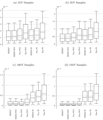
In this section we consider the utility of minimising this concentration inequality as a method of choosing samples from the strata. First we outline the bench-marks used to evaluate our method’s performance. Then we describe two syn-thetic data sets and report the distribution of errors under our method and the benchmarks. Following this, in Section6, our method is evaluated in an example application — that of calculating the Shapley value of a cooperative game.

5.1. Benchmarks algorithms

In the numerical evaluations, we compare the following sampling methods:

• SEBM-WO(Stratified empirical Bernstein method without replacement): our method of iteratively choosing samples from strata to minimize our concentration inequality, Equation (8). An initial sample of two data points from each strata is used to initialise the sample variances of each, with additional samples made to maximally minimise the inequality at each step, before recomputing sample variances. All samples are drawn withoutreplacement, and the inequality used involved the judicious use of martingale inequality lemma9 (see the notice in Section3.1).

• SEBM-W(Stratified empirical Bernstein method with replacement): as above, with the exception that all samples are drawn with replacement, and consequently the inequality does not utilize the martingale inequality given in lemma9.

• Sim-WO(Simple random sampling without replacement): simple random sampling from the population irrespective of stratawithout replacement.

• Sim-W(Simple random sampling with replacement): simple random sam-pling from the population irrespective of stratawith replacement.

• Ney-WO(Neyman sampling without replacement): the method of max-imally choosing sampleswithout replacement from strata proportional to the strata variance.

• Ney-W (Neyman sampling with replacement): the method of choosing sampleswith replacement proportional to the strata variance.

Note that the last three methods assume prior perfect knowledge of the variance of each of the strata, and that in Equations (8) and (5) we selected for minimising a 50% confidence interval (i.e.p= 0.5 andt= 0.5 respectively).

Between these methods there are compared different factors such as the dy-namics of sampling: with and without replacement, with stratification and with-out, between our method and Neyman sampling, and with and without perfect knowledge of stratum variances. For these methods we consider the effectiveness against Beta distributed data and Uniform & Bernoulli data.

5.2. Synthetic Data

The first way we demonstrate the efficacy of our method is to generate sets of synthetic data, and then numerically examine the distribution of errors gen-erated by different methods of choosing finite sequences of samples. In this subsection, we described the two types of synthetic data sets used in this eval-uation, namely: (i) beta distributed stratum data, and (ii) a particular form of uniform and Bernoulli distributed stratum data.

5.2.1. Beta-Distributed Data

The first pool of synthetic data sets are intended to be representative of potential real-world data. These sets have between 5 and 21 strata, with the number of strata drawn with uniform probability, and each strata sub-population has sizes ranging from 10 to 201, also drawn uniformly. The data values in each strata are drawn from beta distributions:

φ(x)_{α,β}=

Γ(α+β) Γ(α)Γ(β)x

α−1₍₁

−x)β−1

(a) 10N Samples

SEBM*

SEBM-W

O

Ney-W

O

Sim-W

O

SEBM-W

Ney-W Sim-W 0

1 2 3 4 5

·10−2

(b) 50N Samples

SEBM*

SEBM-W

O

Ney-W

O

Sim-W

O

SEBM-W

Ney-W Sim-W 0

0.5 1 1.5 2

·10−2

(c) 100N Samples

SEBM*

SEBM-W

O

Ney-W

O

Sim-W

O

SEBM-W

Ney-W Sim-W 0

0.5 1 1.5

·10−2

(d) 150N Samples

SEBM*

SEBM-W

O

Ney-W

O

Sim-W

O

SEBM-W

Ney-W Sim-W 0

0.5 1 1.5

·10−2

5.2.2. A Uniform and Bernoulli Distribution

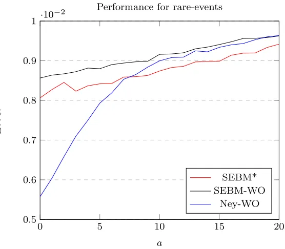
The aim of this section is to examine cases of distributions in which our sam-pling method (SEBM-WO) performs poorly, particularly compared to Neyman sampling (Ney-WO). For this purpose, a data set with two strata is generated, with each stratum containing 1000 points. The data in the first stratum is uni-form continuous data in range [0,1], while the data in the second is all zeros except for a specified small number, a, of successes with value one. For this estimation problem, we conduct stratified random sampling with a budget of 300 samples, comparing the SEBM*, SEBM-WO and Ney-WO methods. The average error returned by the methods across 20000 realisations of this problem, plotted against the number of sucessesa, are shown as a graph in Figure2.

This figure demonstrates that SEBM-WO and SEBM* perform poorly when the strata contain only very small numbers of sucesses. This under-performance is not simply a result of the SEBM-WO method oversampling in a process of learning the stratum variances, as the under-performance is present in SEBM* as well. The reasons for this under-performance are discussed in conjunction with other results in more detail in Section7.

Next, we considered the calculation of the Shapley value as an example ap-plication of our stratified sampling method.

0 5 10 15 20

0.5 0.6 0.7 0.8 0.9

1·10

−2

a

E

r

r

or

Performance for rare-events

SEBM* SEBM-WO

Ney-WO

6. Shapley Value Approximation

The Shapley value is a cornerstone measure in cooperative game theory. It is an axiomatic approach to allocating a divisible reward or cost between partici-pants, where there is a clearly defined notion of how much reward any group (or ‘coalition’) of participants could achieve by themselves (Chalkiadakis, Elkind and Wooldridge, 2012). The Shapley value has many applications, including analysing the power of voting blocks in weighted voting games (Bachrach et al., 2009), in cooperative cost and surplus division problems (Aziz et al., 2016; Chapman, Mhanna and Verbiˇc,2017), and as a measure of network centrality (Michalak et al.,2013).

Formally, a cooperative game, (N, v) ∈ GN, comprises a set of n players, N = {1,2, . . . , n}, and a characteristic function, v : S ⊂ N → R, which is a

function specifying the reward which can be achieved if a subset of the players S⊂N cooperate, wherev(∅) = 0. In this context the Shapley value is a unique allocation which satisfies the following set of natural axioms:

• Efficiency: That the total reward is divided up:P

iψ(hN, vi)i=v(N)

• Symmetry: If two playersiandjare totally equivalent ‘substitutes’ then the receive the same reward: ie. if v(S∪i) =v(S∪j) ∀S ⊆N\ {i, j}, thenψ(hN, vi)i=ψ(hN, vi)j

• Null Player: If the addition of a playerito any coalition brings nothing, and is a ‘null player’, then it receives reward of zero: i.e if v(S∪i) = v(S) ∀S⊆N thenψ(hN, vi)i= 0

• Additivity: That for any two games the reward afforded each player is each is the sum of the games considered together: i.e. for anyv1 andv2, that:ψ(hN, v1+v2i) =ψ(hN, v1i) +ψ(hN, v2i)

Specifically, the Shapley value is a mapping from cooperative games to the player rewards: Sh,_GN →Rn, given by:

Shi((N, v)) = X

S⊂N,i /∈S

(n− |S| −1)!|S|!

n! (v(S∪ {i})−v(S)) (9)

That is, under the Shapley value each player is afforded their average marginal contribution across every possible sequence of player join orderings. Alterna-tively, ifvi,kis the average marginal contribution of playeriacross coalitions of sizek:

vi,k= X

S⊂N

|S|=k, i /∈S

(n− |S| −1)!|S|!

n! (v(S∪ {i})−v(S)), (10)

then the Shapley value can be expressed as:

Shi((N, v)) = 1 n

n−1 X

k=0

Though the Shapley value is conceptually simple, its use is hampered by the fact that its total expression involves exponentially many evaluations of the charac-teristic function (there aren×2n−1_{possible marginal contributions betweenn} players).

However, since the Shapley value is expressible as an average over averages by Equation (11), it is possible to approximate these averages via sampling tech-niques, and particularly so as these averages are naturally stratified by size. In previously published literature, other techniques have been used to allocate sam-ples in this context, particularly simple sampling (Castro, G´omez and Tejada, 2009), Neyman allocation (Castro et al.,2017;O’Brien, Gamal and Rajagopal, 2015), and allocation to minimize Hoeffding’s inequality (Maleki et al.,2013). We assess the benefits of using our bound by comparing its performance to the approaches above in the context of some example cooperative games, as described below.

Example Game 1(Airport Game). Ann= 15player game with characteristic function:

v(S) = max i∈S wi

wherew={w1, . . . , w15}={1,1,2,2,2,3,4,5,5,5,7,8,8,8,10}. The maximum marginal contribution is10, so we assignDi= 10for all i.

Example Game 2(Voting Game). Ann= 15player game with characteristic function:

v(S) = (

1, if P

i∈Swi> P

j∈Nwj/2 0, otherwise

wherew={w1, . . . , w15}={1,3,3,6,12,16,17,19,19,19,21,22,23,24,29}. The maximum marginal contribution is1, so we assignDi= 1 for alli.

Example Game 3 (Simple Reward Division). An n = 15 player game with characteristic function:

v(S) = 1 2

X

i∈S wi 100

!2

wherew={w1, . . . , w15}={45,41,27,26,25,21,13,13,12,12,11,11,10,10,10} The maximum marginal contribution is1.19025, so we assignDi= 1.19025 for alli.

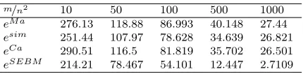
Example Game 4(Complex Reward Division). Ann= 15player game with characteristic function:

v(S) = X i∈S

wi 50

!2

−

$ X

i∈S wi 50

%2

For each game, we compute the exact Shapley value, and then the average error in the approximated Shapley value for a given budgetmof samples. The results are shown in Table 1, where the average absolute error in the Shapley value is computed by sampling with Maleki’s method (Maleki et al., 2013) is denoted eM a_{, e}sim _{is Castro’s simple sampling method (Castro, G´omez and} Tejada,2009),eCa _{is Castro’s Neyman sampling method (Castro et al.,2017),} andeSEBM _{is the error associated with our method, SEBM-WO. The results in} Table1show that our method performs well across the benchmarks. A discussion of all of the results is considered in the next section.

(a) Airport Game average errors

m_/n2 _{10 50 100 500 1000}

eM a _{298.36 133.07 99.639 41.963 29.257}

esim _{357.84 146.09 106.22 44.545 36.333}

eCa _{325.65 115.73 75.85 31.014 22.115}

eSEBM _{259.24 73.754 54.756 7.7099 1.3038}

(b) Voting Game average errors

m_/n2 10 50 100 500 1000

eM a _{130.98 57.775 41.522 18.657 13.178}

esim _{145.72 59.716 40.306 17.563 12.835}

eCa _{142.1 47.35 31.048 14.08 9.7998}

eSEBM 122.79 47.435 33.179 8.5464 1.9953

(c) Simple Reward Division Game average errors

m_/n2 _{10 50 100 500 1000}

eM a 25.678 11.615 7.7921 3.4805 2.2904

esim _{22.102 9.0445 6.2178 2.6419 1.9379}

eCa 22.367 8.925 6.6915 2.7267 1.9402

eSEBM _{19.254 7.0441 5.1578 1.1825 0.28173}

(d) Complex Reward Division Game average errors

m_/n2 10 50 100 500 1000

eM a _{276.13 118.88 86.993 40.148 27.44}

esim 251.44 107.97 78.628 34.639 26.821

eCa _{290.51 116.5 81.819 35.702 26.501}

eSEBM _{214.21 78.467 54.101 12.447 2.7109}

7. Discussion

From the results across Figures1and2and Table1, the main observation is that our sampling technique, SEBM-WO or SEBM-W, performs competitively to Neyman sampling (Ney-WO or Ney-W). This is despite SEBM not having access to knowledge of strata variances, which the Neyman methods do. If instead we compare SEBM*, which has access to strata variances, and Ney-WO then both methods use the same information, and the results are even more positive for our method. The reasons for this performance are interesting, and we now discuss them in more detail.

To begin, from Figure1, observe that sampling without replacement always performs better than sampling with replacement for the same method. This improvement is magnified as the number of samples grows large relative to the size of the population. At the same time, simple random sampling almost always performs worst, because it fails to take advantage of any variance information. These results are as expected.

Next, note that the results of Figure 1 show that there is a mid-range of sample sizes where choosing a different method can have a greater impact on sampling efficiency and rate of average error reduction than the difference be-tween sampling with or without replacement. This is an important insight, as sampling real-world data (e.g. surveys, polling, destructive testing, etc) can be an expensive and slow process. Accordingly an appropriate method of choosing numbers of samples can lead to a material difference in cost for the same accu-racy. There is also a slight decrease in the performance of SEBM* in comparison with Ney-WO in the case of high number of samples and sampling without re-placement, as illustrated in Figure 1. This potentially indicates that lemma 9 can be improved — as noted in Section3.1.

Furthermore, if the data features very rare events, then SEBM-WO and SEBM* seem to perform in a manner less than ideal. These condition are il-lustrated in Figure2, where the more rare the Bernoulli variable successes, the worse our methods perform in comparison with Neyman sampling (Ney-WO). This shortcoming can be partly explained by noting that SEBM-WO unnec-essarily wastes samples on the Bernoulli stratum of rare events in the process of learning that the variance is almost zero, whereas Ney-WO can avoid this because it has prior knowledge of the variances to begin with. As such, this factor accounts for the difference between the performance of SEBM-WO and SEBM* in the context of Figure 1 and also in Figure 2. What is surprising is how small the difference in performance between SEBM-WO and SEBM* is. This indicates that as additional samples are taken that uncertainty about the strata variances have less and less effect upon the total numbers of samples that are eventually drawn from each of the strata.

σ2 P(X≥t)

t= 0.1

t= 0.5

t= 0.9

0.25 0

1.0

Fig 3: The plots againstσ2_of

P(X≥t)≤minsE[exp(sX)] exp(−st)

withE[exp(sX)] via Equations (1) (black)

and (3) (blue) with D = 1. Note that Equation (3) generally captures the rele-vant shape and magnitude of the more ac-curate equation except in region of small σ2_{where the bound is overly weakened.}

minimise. Figure3illustrates how the approximation (2) loosens the bound with respect to the variance. Observe that when the variances are very small that Equation (3) overly loosens the bounds, causing oversampling of strata with very small variances. It appears that this factor is at play in the under-performance shown in Figure2 and also the slight under-performance of our method in the Voting Game in Table1b. We note that there may be other corner-cases where our method also under-performs.

In comparison to existing approaches to approximating the Shapley value, our sampling method shows improved performance on almost all accounts, as shown in Table1. This was particularly the case in the context of large sample budgets, as our method (SEBM-WO, with erroreSEBM_{) sampled without replacement,} while the other methods sampled with replacement. However it would be remiss not to mention the computational overhead of iteratively minimising (one sam-ple at a time) our inequality in the context of our simsam-ple examsam-ple games. This overhead can, in practice, reduce the benefit of using a more efficient sampling method. However, on more complicated games where the characteristic function is slower to calculate, any overhead associated with the sampling choice will be much less relevant. We also note that our method’s performance could poten-tially be further improved by selecting more refinedDi values for our example games.

One primary limitation of our method is that it rests on assumption of known data widthsDi(and in the case of sampling-without-replacement, also on strata sizes Ni), which may not be exactly known in practice. One way to overcome this may be to use our method with a reliable overestimate these parameters (by expert opinion or otherwise). This approximation or estimation may itself open consideration of other probability bounds and/or sampling methods, however we have not investigated this line of inquiry.

of the inequality and not necessarily its magnitude or accuracy as a bound. Our concentration inequality, Equation (8), is derived by a combination of Chernoff bounds fused together with probability unions, so it is expected to give con-servative confidence intervals on the error of the estimate in stratified random sampling, which may be useful outside of the context of sampling decisions.

8. Multidimensional Extension

The method of choosing samples can be extended to multidimensional data by a simple modification.

Specifically, instead of considering data that is single-valued, we consider data points that are vectors. Formally, fornstrata of finite data points which are all vectors of sizeM, let ni be the number of data points in the ith stratum. Let the data in theith stratum have a mean vector valuesµi (withµi,j for thejth component of the vector), which are value bounded within a finite widthDi,j, and have vector value variances σ2

i,j. Given this, if Xi,1, Xi,2, . . . , Xi,ni (with

Xi,1,j being the jth component of such a vector) are vector random variables corresponding to those data values randomly and sequentially drawn (with or without) replacement, then denote the average of the firstmi of these random variables by Ξi,m_i = _m1

i

Pmi

j=1Xi,j (with Ξi,mi,j being the jth component of

that vector average). Let ˆσˆ2_i,j = _mi

i−1

Pmi

k=1(Xi,k,j−Ξi,mi,j)

2 _{be the unbiased} sample variance of the firstmi of these random variables in thejth component. And again, assume we have weightsτi for each stratum.

In this context we have the following theorem:

Theorem 5(Vector SEBM bound). In the context above, then with Ωni

mi,Ψ

ni

mi

per lemma7:

P   PM j=1( Pn

i=1τi(Ξi,mi,j −µi,j))

2

≥

log(6/p)PM_j=1

αni

mi,j+

q βni

mi,j+

q γni

mi,j

2 

≤M p (12)

where:

αni

mi,j =

n X i=1 4 17Ω ni

miD

2 i,jτ

2 i

βni

mi,j = log(3/p)

max i τ 2 iΨ ni mi 2 D_i,j2

γni

mi,j =2

n X

i=1

τi2Ψnmii(mi−1)ˆσˆ

2

i,j/mi+ log(6n/p) X

i

τi2D2i,jΩnmiiΨ

ni

mi

Proof. Squaring (8) and applying it specifically to thejth component of all the vectors gives:

P

(Pn_i=1τi(Ξi,m_i−µi))2 log(6/p) ≥α

ni

mi,j+

q βni

mi,j+

q γni

mi,j

2 !

≤p

Taking a series of union bounds (lemma1) overj gives result.

The left hand side of the inequality in (12) is the square euclidean distance between our weighted stratified sample vector estimate Pn_i=1τiΞi,mi and the

true mean stratified vectorPn_i=1τiµi. In this context a sampling process consists (the same as before) of sampling to maximally minimise the right hand side of the inequality. This formulation can potentially be applied to more involved computational tasks and sampling data with multiple features.

9. Future Work and Applications

We begin this section with a discussion of the relationship of our bound to existing concentration inequalities, and some opportunities for future improve-ments. The derivation of our inequality extends from consideration of Chernoff bounds and probability unions in a similar vein to other EBB derivations (Mau-rer and Pontil,2009;Bardenet and Maillard,2015). However, the bounds on the moment generating functions that we developed in Section3are rife with loos-ening approximations, and stronger and/or more representative bounds could be developed at the cost of greater mathematical complexity. Alternatively, the approach used to derive the Entropic (Boucheron, Lugosi and Massart, 2003) or Effron-Stein methods (Efron and Stein, 1981) could result in different and possibly tighter results.

Additionally, although our method works generally, there may be better or more appropriate sampling methods in the event that there is more information known about the underlying distributions. It is sometimes possible to derive ideal concentration inequalities in restricted circumstances, and more broadly there exist some computational methods to numerically derive ideal bounds (Owhadi et al.,2013;Han et al.,2015). Using these techniques it may be possible to derive ideal numerical bounds, particularly for bounds considering very small numbers of samples.

responsive and interconnected to the network. Because of this, there are various emerging schemes of how a future distribution-network energy market platform might be designed. Within this context, the Shapley value has been proposed as a fair mechanism for the allocation of resources and costs on such networks. The Shapley value has been considered in different ways as a mechanism for pricing demand response (O’Brien, Gamal and Rajagopal, 2015), demand or load (Chapman, Mhanna and Verbiˇc,2017), supply or generation (Acu˜na et al., 2018), and potentially all simultaneously (Burgess, Chapman and Scott,2018). Although computing the Shapley value exactly is impractical in these contexts, sample-based approximations are a promising avenue for implementing Shapely value pricing schemes in real-world electricity systems.

Second, a potential use of our stratified sampling method is in improving the performance of stochastic gradient decent (SGD) methods for training neural networks (Ruder,2016). Neural networks are trained by iteratively refining their parameters — the weights and biases of the network — against a cost function of the network’s performance against training data. One common method of training neural networks is gradient decent (GD). In each iteration of GD, the derivative of how much a change in any parameter would influence the average performance of the network across the training data is calculated as a gradient vector. Once this vector is calculated, each network parameter takes a small step in the direction of this gradient, to incrementally increase the performance of the network, and through many of these steps the network becomes trained. However in many cases, the entire corpus of training data is not used in each iteration but only a fraction of the corpus is sampled (as a ‘batch’ or ‘minibatch’), and the average gradient vector of improved performance across the samples of the batch is calculated as an approximation of the true gradient vector. This iterative process can be broadly called SGD, where one of the hyperparameters is the size of the batches, see Keskar et al. (2017); Smith, Kindermans and Le(2018). In the context of supervised learning, each element of the training data is labelled with the desired output of the neural network for it, and these labels can serve to naturally stratify the training data; or the data can be stratified by other means too (Zhang, Kjellstr¨om and Mandt,2017; Zhang et al., 2019; Zhao and Zhang, 2014). In this setting, Equation 12 may be used to choose between samples of labelled training data, in order to sample batches that more-efficiently estimate of the performance gradient, and hence improve the efficiency of neural network training procedure. This idea of ‘smart sampling’ for neural network training is not particularly new, and our method is compatible with other performance-enhancing techniques in the literature on neural networks (Papa, Bianchi and Cl´emen¸con,2015;Clmenon et al.,2015).

Full exploration of these potential applications are beyond the scope of this document and are left for future work. However, at present, we are pleased to present our analytic concentration inequality (Equation 8) as an immediately computable expression and practical method for choosing samples from strata, and all sourcecode is available at:

x ex

αx2_+βx+γ

c f d

Fig 4:fitting a parabola above an exponential curve for allc≤x≤d

Appendix A: Parabola Fitting

In selecting anα, β, γas the parameters1_{of a parabola αx}2_{+βx+γ≥exp(x)} for allc≤x≤dwhich minimiseszα+γ for constantsc, d, z.

We witness that such a parabola may tangentially touch the exponential curve at one point (atx=f < d) and intersect it at another (atx=d), as illustrated in Figure4.

The parabola’s intersection atx=dand its tangential intersection atx=f can be written in matrix algebra:



 α β γ 

= 



d2 _{d 1} f2 _{f 1} 2f 1 0 



−1

 exp(d) exp(f) exp(f) 



which gives our parabola parameters α, β, γ in terms of f and d, hence our objective functionzα+γ can be written as:

zα+γ=((z+f d−d)(f−d−1)−d)e

f _{+ (f}2_+z)ed

(d−f)2

sincedis fixed, minimising with respect tof givesf = −z

d where our objective function becomes:

zα+γ=ze

d_+d2_e−z/d

z+d2 .

1_{Here we carry the derivation with the explicit dependence on thes (seen in lemma5)}

References

Audibert, J.-Y.,Munos, R.andSzepesv´ari, C.(2007). Tuning Bandit Al-gorithms in Stochastic Environments. In Proc 18th Int. Conf. Algorithmic Learning Theory (ALT‘07) (_{M. Hutter}, _{R. A. Servedio} and _E. Taki-moto, eds.) 150–165. Springer Berlin Heidelberg, Berlin, Heidelberg. Audibert, J.-Y., Munos, R. and Szepesv´ari, C. (2009).

Exploration-exploitation tradeoff using variance estimates in multi-armed bandits.Theor. Comput. Sci.4101876–1902.

Aziz, H.,Cahan, C.,Gretton, C.,Kilby, P.,Mattei, N.andWalsh, T. (2016). A study of proxies for shapley allocations of transport costs.Journal of Artificial Intelligence Research56573-611.

Bachrach, Y., Markakis, E., Resnick, E., Procaccia, A. D., Rosen-schein, J. S.andSaberi, A.(2009). Approximating power indices: theoret-ical and empirtheoret-ical analysis.Autonomous Agents and Multi-Agent Systems20 105-122.

Bardenet, R. and Maillard, O.-A. (2015). Concentration inequalities for sampling without replacement.Bernoulli211361–1385.

Bennett, G.(1962). Probability Inequalities for the Sum of Independent Ran-dom Variables.Journal of the American Statistical Association57 33–45. Bentkus, V.and van Zuijlen, M. (2003). On Conservative Confidence

In-tervals.Lithuanian Mathematical Journal43141–160.

Borgan, O., Langholz, B., Samuelsen, S. O., Goldstein, L. and

Pogoda, J.(2000). Exposure Stratified Case-Cohort Designs.Lifetime Data Analysis639–58.

Boucheron, S.,Lugosi, G.andMassart, P.(2003). Concentration inequal-ities using the entropy method.The Annals of Probability311583-1614. Breslow, N. E.,Hu, J.andWellner, J. A.(2015). Z-estimation and

strat-ified samples: application to survival models.Lifetime Data Analysis21493– 516.

Burgess, M. A., Chapman, A. C. andScott, P. (2018). The Generalized N&K Value:An Axiomatic Mechanism for Electricity Trading.Proc. 17th Int. Conf. Autonomous Agents and Multiagent Systems (AAMAS‘18) 17 1883– 1885.

Carpentier, A., Lazaric, A., Ghavamzadeh, M., Munos, R. and

Auer, P. (2011). Upper-confidence-bound Algorithms for Active Learning in Multi-armed Bandits. InProc. 22nd Int. Conf. Algorithmic Learning The-ory (ALT’11)189–203. Springer-Verlag, Berlin, Heidelberg.

Castro, J.,G´omez, D.andTejada, J.(2009). Polynomial calculation of the Shapley value based on sampling.Computers & OR361726–1730.

Castro, J.,Gmez, D.,Molina, E.andTejada, J.(2017). Improving poly-nomial estimation of the Shapley value by stratified random sampling with optimum allocation.Computers & Operations Research82180 - 188. Chalkiadakis, G.,Elkind, E.andWooldridge, M.(2012).Computational

Chapman, A. C., Mhanna, S. and Verbiˇc, G. (2017). Cooperative game theory for non-linear pricing of load-side distribution network support. In Proc. 10th Bulk Power Systems Dynamics and Control Symposium (IREP‘17).

Clmenon, S.,Bellet, A., Jelassi, O. and Papa, G. (2015). Scalability of Stochastic Gradient Descent based on Smart Sampling Techniques.Procedia Computer Science53 308-315.

Efron, B.andStein, C.(1981). The Jackknife Estimate of Variance.Annals of Statistics9586–596.

´

Etor´e, P.andJourdain, B.(2010). Adaptive Optimal Allocation in Stratified Sampling Methods. Methodology and Computing in Applied Probability 12 335–360.

Han, S.,Tao, M.,Topcu, U.,Owhadi, H.andMurray, R.(2015). Convex Optimal Uncertainty Quantification.SIAM Journal on Optimization25 1368-1387.

Hillson, R., Alejandre, J. D., Jacobsen, K. H., Ansumana, R.,

Bockarie, A. S.,Bangura, U.,Lamin, J. M.andStenger, D. A.(2015). Stratified Sampling of Neighborhood Sections for Population Estimation: A Case Study of Bo City, Sierra Leone.PLoS ONE10e0132850.

Hoeffding, W.(1963). Probability Inequalities for Sums of Bounded Random Variables.Journal of the American Statistical Association5813–30.

Horvitz, D. G.andThompson, D. J.(1952). A Generalization of Sampling Without Replacement From a Finite Universe.Journal of the American Sta-tistical Association47663–685.

Hu, W.,Cai, J.andZeng, D.(2014). Sample size/power calculation for strat-ified casecohort design.Statistics in Medicine33 3973–3985.

Keskar, N. S., Mudigere, D., Nocedal, J., Smelyanskiy, M. and

Tang, P. T. P. (2017). On Large-Batch Training for Deep Learning: Gen-eralization Gap and Sharp Minima. International Conference on Learning Representations.

Khan, M. G. M., Ahmad, N. and Khan, S. (2009). Determining the Op-timum Stratum Boundaries Using Mathematical Programming. Journal of Mathematical Modelling and Algorithms8409–423.

Kozak, M.(2004). Optimal stratification using random search method in agri-cultural surveys.Statistics in Transition 6797–806.

Legg, J. C.andFuller, W. A.(2009). Chapter 3 - Two-Phase Sampling. In Handbook of Statistics, (C. R. Rao, ed.).Handbook of Statistics 29 55 - 70. Elsevier.

Maleki, S., Tran-Thanh, L., Hines, G., Rahwan, T. and Rogers, A. (2013). Bounding the Estimation Error of Sampling-based Shapley Value Ap-proximation.arXiv e-printsarXiv:1306.4265.

Maurer, A. (2006). Concentration inequalities for functions of independent variables.Random Structures and Algorithms29121-138.

and_{Jennings, N. R.}(2013). Efficient Computation of the Shapley Value for Game-theoretic Network Centrality.J. Artif. Int. Res.46607–650.

Miratrix, L. W.andStark, P. B.(2009). Election Audits Using a Trinomial Bound.IEEE Transactions on Information Forensics and Security4974–981. Mnih, V.,Szepesv´ari, C.andAudibert, J.-Y.(2008). Empirical Bernstein

Stopping. In Proc. 25th Int. Conf. Machine Learning. ICML ’08 672–679. ACM, New York, NY, USA.

Acu˜na, L. G., R´ıos, D. R., Arboleda, C. P.and Ponz´on, E. G. (2018). Cooperation model in the electricity energy market using bi-level optimization and Shapley value.Operations Research Perspectives 5161–168.

Neyman, J. (1938). Contribution to the Theory of Sampling Human Popula-tions.Journal of the American Statistical Association33101-116.

O’Brien, G., Gamal, A. E.andRajagopal, R. (2015). Shapley Value Es-timation for Compensation of Participants in Demand Response Programs. IEEE Transactions on Smart Grid62837–2844.

Owhadi, H., Scovel, C., Sullivan, T. J., McKerns, M. and Ortiz, M. (2013). Optimal Uncertainty Quantification.SIAM Rev55271–345.

Papa, G., Bianchi, P. and Cl´emenc¸on, S. (2015). Adaptive Sampling for Incremental Optimization Using Stochastic Gradient Descent. InProc. 25th Int. Conf. Algorithmic Learning Theory (ALT‘15)(_{K. Chaudhuri},_C. GEN-TILE and S. Zilles, eds.) 317–331. Springer International Publishing, Cham.

Prentice, R. L.(1986). A case-cohort design for epidemiologic cohort studies and disease prevention trials.Biometrika731-11.

Rehman, M. Z., Li, T.and Li, T.(2012). Exploiting empirical variance for data stream classification.Journal of Shanghai Jiaotong University (Science) 17245–250.

Ruder, S. (2016). An overview of gradient descent optimization algorithms. arXiv e-printsarXiv:1609.04747.

Saegusa, T. and Wellner, J. A. (2013). Weighted likelihood estimation under two-phase sampling.The Annals of Statistics41269–295.

Serfling, R. J.(1974). Probability Inequalities for the Sum in Sampling with-out Replacement.The Annals of Statistics239–48.

Smith, S. L., Kindermans, P.-J. and Le, Q. V. (2018). Don’t Decay the Learning Rate, Increase the Batch Size. InInternational Conference on Learn-ing Representations.

Stark, P. B.(2009). Risk-limiting Postelection Audits: Conservative P-values from Common Probability Inequalities. IEEE Transactions on Information Forensics and Security41005–1014.

Thomas, P. S., Theocharous, G. and Ghavamzadeh, M. (2015).

High-Confidence Off-Policy Evaluation. InProc. 29th AAAI Conf. Artificial Intel-ligence, January 25-30, 2015, Austin, Texas, USA.3000–3006.

Wright, T.(2012). The Equivalence of Neyman Optimum Allocation for Sam-pling and Equal Proportions for Apportioning the U.S. House of Representa-tives.The American Statistician66217–224.

Imbalanced Data: Determinantal Point Processes for Mini-batch Diversifica-tion. InProc. Conf. Uncertainty in Artificial Intelligence (UAI‘17).

Zhang, C., Oztireli, C.¨ , Mandt, S. and Salvi, G. (2019). Active Mini-Batch Sampling using Repulsive Point Processes. InProc. 33rd AAAI Conf. Artificial Intelligence (AAAI‘19, accepted).