New candidates for multivariate trapdoor functions

New candidates for multivariate

trapdoor functions

Jaiberth Porras

,

John B. Baena

,

Jintai Ding

1

_{Universidad Nacional de Colombia, Medell´ın, Colombia}

2

_{University of Cincinnati, Cincinnati, OH, USA}

Abstract.We present a new method for building pairs of HFE polynomials of

high degree, such that the map constructed with such a pair is easy to invert. The inversion is accomplished using a low degree polynomial of Hamming weight three, which is derived from a special reduction via Hamming weight three polynomials produced by these two HFE polynomials. This allows us to build new candidates for multivariate trapdoor functions in which we use the pair of HFE polynomials to fabricate the core map. We performed the security analysis for the case where the base field is GF(2) and showed that these new trapdoor functions have high degrees of regularity, and therefore they are secure against the direct algebraic attack. We also give theoretical arguments to show that these new trapdoor functions overGF(2) are secure against the MinRank attack as well.

Key words and phrases. Multivariate cryptography, HFE polynomials, HFE cryptosystem, trapdoor functions, Zhuang-zi algorithm.

1. Introduction

The public key cryptosystems currently used in practice are based on the diffi-culty of factoring large integers or solving the Discrete Logarithm Problem. In 1996 P. Shor published an algorithm to solve both problems in polynomial time on a quantum computer [17]. Some experts argue that it is possible to build in the coming years a quantum computer, which is a threat to our modern com-munication system. This leads to the recent fast development of Post-Quantum Cryptography . Post-Quantum Cryptography refers to the study of cryptosys-tems that have the potential to resist the possible future quantum computer attacks [1].

Multivariate Public Key Cryptography (MPKC) is part of the Post-Quantum Cryptography. In MPKC, the public key consists of a set of multivariate quadra-tic polynomials over a finite field. One of the main cryptosystems in MPKC is named Hidden Field Equations (HFE), proposed by Patarin in 1996 [16]. The public key in HFE is formed by “hiding” a core polynomialF by two invertible affine transformations, and using the vector space structure of a field extension of the base field.

A crucial part in HFE is the choice of the degreeD of the core polynomial F. The degree D cannot be too big, since otherwise the decryption process would not be efficient. The main attacks against HFE, direct algebraic attack ([10, 5, 6, 14, 15]) and the Kipnis-Shamir MinRank attack (KS attack [13]), exploit this fact. For characteristic 2, HFE is vulnerable to the direct algebraic attack [10]. Recently, some authors improved the KS attack and were able to break certain HFE systems, over both odd and even characteristic [2].

We propose a special reduction method to construct new candidates for trapdoor functions using HFE polynomials of high degree. The use of these high degree polynomials prevents the known attacks against HFE. This opens the possibility to build a secure variant of the HFE cryptosystem.

The idea of the construction is inspired by the first steps of the Zhuang-Zi algorithm [7]. Given a finite field k of size q and a field extension K of degree n, we consider two high degree HFE polynomials over K of the form F(X) =P_a

ijXq

i_+qj

+P_b

iXq

i

+cand ˜F(X) =P_˜a

ijXq

i_+qj

+P_˜b

iXq

i

+ ˜c, where the coefficients aij, bi, c,˜aij,˜bi,˜c ∈ K are to be determined. The idea

behind the method is to construct a low degree polynomial Ψ of Hamming weight three of the form

Ψ =Xα1F0+· · ·+αnFn−1+β1F˜0+· · ·+βnF˜n−1

+

Xqαn+1F0+· · ·+α2nFn−1+βn+1F˜0+· · ·+β2nF˜n−1

,

where F0, F1,· · · , Fn−1 are the Frobenius powers of F, and ˜F0,F˜1,· · · ,F˜n−1

are the Frobenius powers of ˜F.

To obtain such a polynomial Ψ we need to determine the coefficients of F and ˜F, also the scalars αi and βi, such that the degree of Ψ is less than or

equal to a fixed positive integerD0 (the integerD0 is such that we can easily

invert Ψ using Berlekamp’s algorithm). To achieve this, we derive a system of equations from the vanishing coefficients of the terms in Ψ of degree higher thanD0. After randomly choosing in this system the scalarsαiandβi, we get

a linear system with more variables than equations, and thus we can guarantee nontrivial solutions for it. This linear system has aboutn3_{variables and}

there-fore we have to deal with huge matrices to reach large values ofn. On the plus side we have that these matrices are sparse, which is an advantage in terms of efficiency.

The new multivariate trapdoor function is built in a similar way to the HFE scheme (composition with invertible affine transformations), except that now the core map is replaced by the mapG= (F,F˜). The main part of the inversion of the trapdoor function is to invert the map G, which is achieved using the low degree Hamming weight three polynomial Ψ and the scalarsαi, βi.

function has high degree of regularity, very different from what was observed by Faug`ere and Joux [10] for a system of quadratic equations derived from a single HFE polynomial with low degree. For the case of q = 2, our extensive experiments confirmed that the new trapdoor function has high degree of re-gularity (it increases asnincreases). This high degree of regularity shows that our new candidates for multivariate trapdoor functions are secure against the direct algebraic attack.

Furthermore, for the case of q = 2, we can give a theoretical argument to show why the MinRank attack does not work against the new trapdoor functions, based on some results about the degree of regularity obtained by Ding and Hodges [8]. From those results, we see that, for q = 2, it suffices to make sure that our trapdoor function has a high degree of regularity to conclude that both the direct algebraic and KS MinRank attacks do not work against these new trapdoor functions. We show that this is indeed the case and that our new trapdoor functions are secure against these two attacks. For larger values ofq, this argument cannot be used and the MinRank attack must be directly performed against these new trapdoor functions.

The method described here was not our first attempt to reduce high degree HFE polynomials along the same line. Among failed attempts, we considered using a single polynomialF, but the linear systems we needed to solve had more equations than variables and then we could not guarantee nontrivial solutions for them. This lead us to use two HFE polynomials instead of one in order to get a linear system with more variables than equations and this gives the construction in this paper.

This paper is organized as follows. First, we present some background ma-terial about HFE cryptosystems. Secondly, we describe the method for building the new candidates for multivariate trapdoor functions. Next, we present a toy example to explain step by step our method, and two big examples. Then, we carry out a security analysis and discuss future work. In the appendix we show some data about the generation of the new trapdoor function.

2. Background

The cryptosystem Hidden Field Equations (HFE) was proposed by Patarin in 1996 [16]. The public key is formed by “hiding” a core polynomial F via two invertible affine transformations, and taking advantage of the vector space structure of an extension of the base field.

Letkbe a finite field of sizeq. Fixn∈_Nand take an irreducible polynomial g over k of degree n. Consider the field extension K = k[y]/(g(y)). Then K∼=kn_{, via the isomorphismϕ:K→k}n _{defined by}

ϕ u1+u2y+. . .+unyn−1

= (u1, u2, . . . , un).

Notice that

We say that a polynomial hasHamming weight W if the maximum of the q-Hamming weights of all its exponents is W. The q-Hamming weight of a non-negative integer is the sum of the q-digits of its q-nary expansion. Let F :K→K be a Hamming weight two polynomial of the form

F(X) =

n−1

X

0≤j≤i

aijXq

i_+qj

+

n−1

X

i=0 biXq

i

+c,

where the coefficients aij, bi, c are chosen randomly inK. Such a polynomial

F is called an HFE polynomial. If in addition, we require that deg(F) ≤D, where D is a fixed positive integer, we say thatF is an HFE polynomial with

boundD.

For a fixedD, an HFE cryptosystem is built as follows. First, we randomly choose an HFE polynomial with boundD, sayF: K→K. Then, we randomly choose two invertible affine transformations S and T over kn. The public key P is the composition ofF with the transformationsSandT, together with the isomorphismϕ, i.e.,

P =T◦ϕ◦F◦ϕ−1◦S.

Notice thatP is ann−tuple of the form

P= (P1(x1, . . . , xn),· · ·, Pn(x1, . . . , xn)),

where eachPiis a multivariate quadratic polynomial. The private key consists

of the core mapF together with the transformationsS andT.

When constructing an HFE cryptosystem we need to be very careful with the choice of the bound D. This bound cannot be too high, since this would affect the decryption process, making it inefficient. Also,Dcannot be too small, because this would make the system vulnerable to the algebraic and KS attacks.

Many attempts have been made to build safe HFE variants for both digital signatures and encryption schemes [12, 9, 4, 11]. However, most of them have not been successful. One of the latest, Multi-HFE [11], proposes to use as core map a system of multivariate polynomials over K, instead of a single HFE polynomial. This cryptosystem was broken by means of a generalization of the Kipnis-Shamir MinRank attack [2].

In the next section we present a procedure to generate a low degree polyno-mial of Hamming weight three, which can be used to invert a map constructed with two high degree HFE polynomials. This idea enables us to build candidates for trapdoor functions using high degree HFE core polynomials, preventing the attacks that we mentioned earlier.

3. Construction of new candidates for multivariate trapdoor functions

The process of decryption involves inverting the mapF (search of pre-images). Therefore, if we take a polynomial of high degree the decryption could be impossible, and if otherwise we take a polynomial of low degree the attacks mentioned above would work.

To overcome this weakness, we developed a method for building pairs of HFE polynomials of very high degree, and such that the map constructed with such a pair is easy to invert, using a low degree polynomial derived from a spe-cial reduction via Hamming weight three polynomials. This low degree polyno-mial is easy to invert by means of Berlekamp’s algorithm. In this way, we are able to use two HFE polynomials of high degree to construct a new candidate for a trapdoor function, and a polynomial of small degree as the trapdoor used to invert such trapdoor function.

3.1. The Reduction method

LetF :K→K and ˜F :K→K be two high degree HFE polynomials of the form

F(X) =

n−1

X

0≤j≤i

aijXq

i_+qj

+

n−1

X

i=0 biXq

i

+c,

˜ F(X) =

n−1

X

0≤j≤i

˜ aijXq

i_+qj

+

n−1

X

i=0

˜ biXq

i

+ ˜c,

where the coefficients aij, bi, c,˜aij,˜bi,˜c ∈ K are to be determined. Next, let

F0, F1,· · ·, Fn−1be the Frobenius powers ofF and let ˜F0,F˜1,· · ·,F˜n−1 be the

Frobenius powers of ˜F, i.e.,

Fi(X) = [F(X)] qi

and ˜Fi(X) =

h

˜ F(X)i

qi

, fori= 0,1,· · ·, n−1.

LetD0 be an upper bound for the degree of a univariate polynomial equation

that can be solved efficiently using Berlekamp’s algorithm.

The key part of this method is to construct a polynomial Ψ of the form

Ψ =Xα1F0+· · ·+αnFn−1+β1F˜0+· · ·+βnF˜n−1

+

Xqαn+1F0+· · ·+α2nFn−1+βn+1F˜0+· · ·+β2nF˜n−1

,

such that deg(Ψ)≤D0. Notice that Ψ is a Hamming weight three polynomial.

To accomplish this, we need to determine the coefficients ofF and ˜F, also the scalars αi and βi, such that the coefficients of the terms in Ψ of degree

vanishing coefficients in Ψ of degree higher than D0. This yields a system of

equations of the form

g1(z1, z2,· · · , zN) = 0,· · ·, gt(z1, z2,· · · , zN) = 0,

where the variablesz1, z2,· · ·, zN are the coefficients ofF and ˜F, together with

the scalarsαi andβi.

The number t of equations of this system depends on how small we want the degree boundD0 to be. More precisely,t is the number of different terms

in Ψ with degree higher thanD0. To invert the trapdoor function, which we

will describe in Section 3.3, via the use of the polynomial Ψ, we require that the polynomial Ψ has degree smaller thanD0.

If we write each variablezj in terms of the basis

1, y,· · ·, yn−1 _{, we obtain}

a system of quadratic equations. More precisely, each variablezj in this system

can be written in the form

zj=u1j+u2jy+· · ·+unjyn−1, (1)

whereu1j,· · · , unj arennew variables. Next, by the linearity of the Frobenius

powers, we get

z_jqi=u1j+u2jyq

i

+· · ·+unjy(n−1)q

i

. (2)

After we write each powerym _{as a linear combination of the elements of the}

basis 1, y,· · · , yn−1 _{with coefficients ink, and group like terms, we get that}

zq_ji =h1j(u1j,· · · , unj) +h2j(u1j,· · · , unj)y2+· · ·+hnj(u1j,· · · , unj)yn−1,

(3) where eachhij is a linear function with coefficients ink.

We now write each variable of the systemg1= 0,· · ·, gt= 0 in the form (1),

and proceed like in (2) and (3). By comparing the coefficients of the elements of the basis1, y, y2,· · · , yn−1 we obtain a system ofnt quadratic equations in n[n(n+ 1) + 6n+ 2] =n3+ 7n2+ 2nvariables overk. These equations are in fact bilinear, i.e., each term of these equations has the product of a variable that comes from the coefficients and a variable that comes from the scalars. Thus, if we randomly fix the variables associated to the scalars we obtain a sparse linear system coming from the coefficients ofF and ˜F. Due to its construction, this linear system has more variables than equations, i.e.,nt < n3_{+ 7n}2_{+ 2n,}

and hence we can always get nontrivial solutions. We then randomly choose one of those solutions to build the high degree polynomialsF and ˜F and the reduced polynomial Ψ of degree less than or equal toD0, as explained above.

3.2. Complexity of the reduction method and dimension of the so-lution space

The described method leads to a sparse linear system over the small field k with more variables than equations. This system has about n3 _{variables and}

thus the complexity of the reduction method is polynomial: O n3ω

, where ω is a constant that depends on the elimination algorithm used to solve the sparse linear system.

On the other hand, after we choose the 4nscalars αi andβi in the system

{gi(z1, z2,· · ·, zN) = 0 :i= 1,· · · , t}, we get a new system over the big fieldK

withtequations andN−4nvariables (the coefficients ofF and ˜F). Therefore, in this new system the number of variables exceeds the number of equations by (N −4n)−t. Hence the final linear system over the small field k has at leastn((N−4n)−t) free variables. Then we have at least qn((N−4n)−t)_{> q}n

possible choices for the coefficients of the polynomials F and ˜F. Thus, if we choose large parametersqandn, and if we randomly choose a solution from the solution space, it is impossible for anyone to guess correctly the polynomials we will use. The large dimension of the solution space also ensures that there are sufficiently many choices for the core map.

3.3. How to build and invert the trapdoor function

For building a new candidate for multivariate trapdoor function, we make use of a map of the formG= (F,F˜) :K→K×K, in whichF and ˜F have been constructed by the method described in Section 3.1. We select two invertible affine transformationsS : kn _→kn _{and T : k}2n _→k2n_{. Similar to HFE, the}

multivariate trapdoor function will be the composition from kn _{to k}2n _given

byP =T◦(ϕ×ϕ)◦G◦ϕ−1◦S (see Figure 1).

K G //K×K

ϕ×ϕ

kn S //

P

5

5

kn //

ϕ−1

O

O

k2n T //k2n

Figure 1.New candidate for multivariate trapdoor function.

The crucial part to invert the trapdoor function is to invert the core map G= (F,F˜), since the transformationsSandT, and the isomorphismϕ, are easy to invert. In what follows we explain how to invertG. Consider an elementX0∈ K and let (Y1, Y2) = G(X0) = (F(X0),F˜(X0)). We show how to recover X0

be the Frobenius powers of ˜F. By the construction of F and ˜F, there exist scalarsα1,· · · , α2n, β1,· · · , β2n such that the polynomial

Ψ =

2

X

j=1 Xqj−1

n

X

i=1

αi+n(j−1)Fi−1+βi+n(j−1)F˜i−1

has degree less than or equal toD0.

We defineF0=F−Y1and ˜F0 = ˜F−Y2, and

Ψ0 =

2

X

j=1 Xqj−1

n

X

i=1

αi+n(j−1)Fi0−1+βi+n(j−1)F˜i0−1.

Clearly,F0(X0) = 0 and ˜F0(X0) = 0, and therefore Ψ0(X0) = 0. Given that

F_i0= (F −Y1)q

i

=Fqi_−Yqi

1 =Fi−Yq

i

1 and ˜Fi0= ( ˜F −Y2)q

i

= ˜Fqi_−Yqi

2 =

˜ Fi−Y

qi

2 , the polynomial Ψ0, just like Ψ, has degree less than or equal to D0, when we choose D0 ≥q. Thus, we can find the roots of Ψ0 by means of

Berlekamp’s algorithm and therefore we can recover the common root X0 of

the polynomialsF0 and ˜F0.

We now discuss the complexity of the trapdoor function inversion. The isomorphism ϕ and its inverse ϕ−1 can be represented in matrix form [2]. Thus, except for the inversion of the core map G, the computational cost of each step of the algorithm to invert the trapdoor function is the cost of a matrix multiplication. The degrees of the polynomials F and ˜F, which are the components of the map G, are extremely high (usually close to qn−1), which makes impossible to invertGdirectly for practical values ofn. However, as noted above, the inversion of the map G can be reduced to finding the roots of the low degree polynomial Ψ0, which can be done efficiently using Berlekamp’s algorithm. For the particular case ofq= 2, in all the computations that we performed we were able to obtain a function Ψ0of degree less than 500, whose roots can be found very quickly using Berlekamp’s algorithm. Therefore, inverting the trapdoor function is a very efficient process.

4. Examples

We now show some examples built by the method described in Section 3.1. We begin by presenting a toy example in which we explain step by step the procedure. We next show two large scale cases.

Example 1. Let q= 2 and n = 2, and consider the field with two elements k=GF(2). We select the irreducible polynomial g(y) =y2_{+y+ 1∈k[y]. A}

the ringK[X]/ Xqn

−X

are of the form

F(X) =a01X3+b0X+b1X2+c,

˜

F(X) = ˜a01X3+ ˜b0X+ ˜b1X2+ ˜c,

wherea01, b0, b1, c,˜a01,˜b0,˜b1,˜c∈K.

The Frobenius powers of F and ˜F, in that order, are:

F0=a01X3+b0X+b1X2+c,

F1=a201X3+b02X2+b21X+c2,

˜

F0= ˜a01X3+ ˜b0X+ ˜b1X2+ ˜c,

˜

F1= ˜a201X 3

+ ˜b20X 2

+ ˜b21X+ ˜c 2

.

We now multiply the Frobenius powers byX andXq and we obtain

XF0=a01X+b0X2+b1X3+cX,

XF1=a201X+b 2 0X

3_+b2 1X

2_+c2_X,

X2F0=a01X2+b0X3+b1X+cX2,

X2F1=a201X 2_+b2

0X+b 2 1X

3_+c2_X2_,

XF˜0= ˜a01X+ ˜b0X2+ ˜b1X3+ ˜cX,

XF˜1= ˜a201X+ ˜b 2 0X

3_{+ ˜b}2 1X

2_{+ ˜c}2_X,

X2F˜0= ˜a01X2+ ˜b0X3+ ˜b1X+ ˜cX2,

X2F˜1= ˜a201X 2_{+ ˜b}2

0X+ ˜b 2 1X

3_{+ ˜c}2_X2_.

Then we form the polynomial Ψ =X(α1F0+α2F1+β1F˜0+β2F˜1) +X2(α3F0+ α4F1+β3F˜0+β4F˜1). In this example we want to determine the coefficients aij, bi, c,˜aij,˜bi,c˜and the scalarsαi, βi such that the terms of degree≥2 in Ψ

vanish. In order to do that, we have to solve the following two equations

α1b0+α2b21+α3(a01+c) +α4 a201+c2

+β1˜b0+β2˜b21

+β3(˜a01+ ˜c) +β4 ˜a201+ ˜c 2

= 0,

α1b1+α2b20+α3b0+α4b21+β1˜b1+β2˜b20+β3˜b0+β4˜b21= 0.

We randomly choose the scalars (α1,· · · , α4) = (0,0, b,1) and (β1,· · · , β4) =

(0, b, b2_{, b}2_{). Then we write the variables a}

01, b0, b1, c,˜a01,˜b0,˜b1,c˜in terms of

the basis 1, y,· · ·, yn−1_{, as follows:}

Proceeding as explained in Section 3.1, we get the linear equations

u1+u7+u10+u14+u16= 0,

u1+u7+u10+u13+u16= 0,

u4+u5+u6+u11+u13= 0,

u3+u4+u6+u13+u14= 0.

One of the solutions of this system is

(u1,· · · , u16) = (0,0,1,1,1,0,1,1,0,1,1,1,1,1,0,1).

This solution leads to the coefficients

(a01, b0, b1, c,a˜01,˜b0,˜b1,˜c) = 0, b2,1, b2, b, b2, b2, b.

With these coefficients we get the polynomialsF =X2+b2X+b2 and ˜F = bX3+b2X2+b2X+b. Then, we use the scalarsαi andβito form the reduced

polynomial Ψ =b2X.

Example 2. In this example, for convenience in the presentation, we consider the coefficients and the scalars in the small field k=GF(2) so we can nicely present the polynomials here. Of course, a realistic example would require the coefficients to be taken in the big fieldK and then the coefficients would not only be ones and zeros. Letq= 2 andn= 17, and consider the field with two elementsk=GF(2). We select the irreducible polynomialy17_+y3_{+ 1∈k[y].}

in the previous example, we obtain the polynomials

F =X98304+X81920+X67584+X66560+X66048+X65664+X65568+

X65552+X65540+X49152+X40960+X33792+X32896+X32832+

X32800+X32772+X32770+X32769+X18432+X16896+X16640+

X16416+X16400+X16392+X16388+X16386+X10240+X8208+

X8192+X6144+X4608+X4352+X4112+X4104+X3072+X2080+

X2064+X2049+X1536+X1152+X1056+X1040+X1028+X1025+

X768+X640+X520+X384+X320+X288+X272+X258+X257+

X192+X136+X132+X130+X96+X68+X66+X36+X34+

X18+X12+X10+X8+X5+X3,

˜

F =X131072+X98304+X81920+X66560+X65664+X65568+X65552+

X65544+X65540+X65538+X33280+X32832+X32784+X32776+

X32770+X17408+X16896+X16640+X16512+X16400+X16392+

X16384+X12288+X10240+X9216+X8704+X8256+X8208+X8200+

X8194+X8193+X8192+X4224+X4160+X4112+X4100+X4097+

X2304+X2176+X2080+X2052+X2049+X1280+X1088+X1056+

X1028+X1025+X768+X576+X544+X528+X520+X514+X512+

X384+X258+X257+X256+X136+X132+X130+X128+X96+

X68+X66+X48+X40+X36+X34+X32+X20+X18+X10+

X6+X3+X2.

The scalars (α1,· · ·, α34) are

(1,1,0,0,0,1,1,0,1,1,0,1,1,0,0,1,1,1,1,0,0,1,0,0,1,0,0,0,0,0,1,0,1,1),

and the scalars (β1,· · ·, β34) are

(1,0,1,0,0,0,0,1,0,1,1,0,0,0,1,1,0,0,0,1,1,1,0,1,0,1,0,0,0,1,1,1,1,0).

These values, together with the polynomials F and ˜F, lead to the reduced polynomial

Ψ =X36+X35+X33+X26+X25+X22+X19+X12+X11+X8.

(F(X0),F˜(X0)) = (b114562, b126611). We now show how to recover X0 from

(Y1, Y2). First we putF0 =F−Y1 and ˜F0= ˜F−Y2 and use the scalarsαiand

βi to form the low degree polynomial

Ψ0=X36+X35+X33+X26+X25+X22+X19+X12+X11+

X8+X5+b117898X2+b101296X.

The set of roots of the polynomial Ψ0, found very quickly by Berlekamp’s al-gorithm, is

0, b51298 _{. Notice that X}

0 is one of these roots.

Example 3. With q = 2 and n = 60, and taking the coefficients and the scalars in the big field K, we found a pair of polynomials F and ˜F with the same degreeD and

log_qD

= 59. The reduced polynomial Ψ that we found has degree 386. Hence, we can invert easily the map G = (F,F˜) via the low degree polynomial Ψ using Berlekamp’s algorithm. These polynomials are too big to be displayed here. In this example we needed to deal with a sparse matrix of size 208080×226800 and the time and memory used were 4.6 days and 52.7 GB, respectively.

5. Security analysis

As we noted before, there are two attacks that have threatened the security of HFE schemes: direct algebraic attack and Kipnis-Shamir MinRank attack. Here we analyze these attacks against the new candidates for multivariate trapdoor functions in the special caseq= 2.

We would like to recall the recent result on the degree of regularity of Ding and Hodges [8]. We know that for an HFE system P the degree of regularity is bounded by

(q−1) Q-Rank(P)

2 + 2,

where Q-Rank(P) is the quadratic rank for the quadratic operator P. So for q= 2 we have that this degree of regularity is bounded by

Q-Rank(P)

2 + 2.

Since the corresponding quadratic rank used in the Kipnis-Shamir MinRank attack is given by Q-Rank(P), we see that if an HFE system has a high degree of regularity, this HFE system must have a high quadratic rank for the Kipnis-Shamir attack. From this we conclude that it suffices to show that our new trapdoor functions have high degree of regularity, in order to demonstrate that the MinRank attack will not work against these new trapdoor functions. We dedicate the rest of this section to discuss the algebraic attack against the new trapdoor functions.

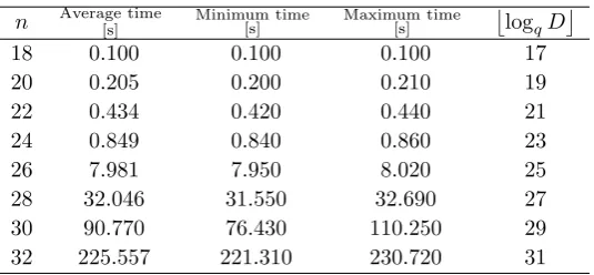
n Average time_[s] Minimum time_[s] Maximum time_[s]

log_qD

18 0.100 0.100 0.100 17

20 0.205 0.200 0.210 19

22 0.434 0.420 0.440 21

24 0.849 0.840 0.860 23

26 7.981 7.950 8.020 25

28 32.046 31.550 32.690 27

30 90.770 76.430 110.250 29

32 225.557 221.310 230.720 31

Table 1.Algebraic attack against the new trapdoor function forq= 2.

(P1, . . . , P2n), i.e., she wants to find a pre-image of an element (y1, . . . , y2n)∈

ImP ⊆k2n. This person only has access to the trapdoor functionP. Attempt-ing to solve directly the system of equations

P1(x1, . . . , xn)−y1= 0

P2(x1, . . . , xn)−y2= 0

.. .

P2n(x1, . . . , xn)−y2n = 0,

(4)

is what we call the direct algebraic attack. One way to do this is with the help of a Gr¨obner basis. We ran extensive experiments using the F4 algorithm of

MAGMA, [3], to perform the direct algebraic attack forq= 2 and several values ofn, on a Sun X4440 server, with four Quad-Core AMD OpteronTM Processor 8356 CPUs and 128 GB of main memory (each CPU is running at 2.3 GHz). For the trapdoor functions used in these experiments we utilized D0 = 500.

The results of our experiments are shown in Table 1 and 2, and Figure 2, 3 and 4. TheF4function of MAGMA is the most efficient implementation of the

Gr¨obnerF4algorithm that is currently available.

In Table 1 and Figure 2 we can observe that the time needed to solve the equations byF4has an exponential growth inn. We can also see this behaviour

with the memory used by theF4algorithm. This situation is different from the

20 25 30 35 40 10−1

100 101 102 103 104 105

n

CPU

time

q= 2

20 25 30 35 40

102 103 104 105

n

Memory

(MB)

q= 2

Figure 2.Algebraic attack against the new trapdoor function forq= 2.

0 10 20 30 40

2 3 4 5

n

Degree

of

regularit

y q= 2

Figure 3.Degree of regularity for the algebraic attack against the new trapdoor

function.

Another evidence that the complexity of the algebraic attack against the new trapdoor functions is exponential, is that the degree of regularity of the trapdoor function increases as n increases. This behaviour can be observed in Figure 3. As we mentioned earlier, the fact that this degree of regularity increases asnincreases, not only says that the direct algebraic does not work against the new trapdoor functions, but also that the Kipnis-Shamir MinRank attack is not successful against these new trapdoor functions.

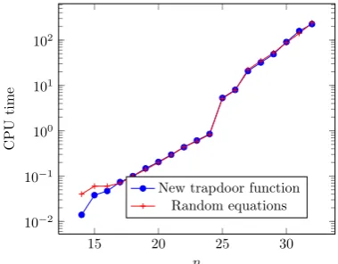
We also chose random quadratic equations of the same dimensions (kn _→

k2n_{) and found that the time needed to solve such equations using Gr¨obner}

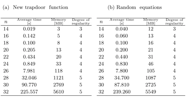
(a) New trapdoor function

n Average time_[s] Memory_{[MB] regularity}Degree of

14 0.019 3 3

16 0.142 5 4

18 0.100 8 4

20 0.205 13 4

22 0.434 20 4

24 0.849 33 4

26 7.981 118 4

28 32.046 1121 5

30 90.770 2769 5

32 225.557 5610 5

(b) Random equations

n Average time_[s] Memory_{[MB] regularity}Degree of

14 0.040 12 3

16 0.060 13 4

18 0.100 16 4

20 0.200 21 4

22 0.440 31 4

24 0.830 46 4

26 7.800 105 4

28 34.700 1087 5

30 87.810 2725 5

32 239.260 5549 5

Table 2.Algebraic attack comparison between the new trapdoor function and

ran-dom equations forq= 2.

In Table 2 we can notice that the degree of regularity of the new trapdoor function is the same as the degree of regularity of the set of random equations. In both cases we observe that the degree of regularity increases asnincreases. From all the information we collected with our experiments, it seems that the F4algorithm is no more efficient in solving the equations from the new trapdoor

function than a set of random equations of the same dimensions. In other words, with respect to the direct algebraic attack, the new trapdoor function behaves as if it were a system of random quadratic equations.

6. Conclusions and future work

We have created a procedure to build candidates for multivariate trapdoor functions using pairs of HFE polynomials of high degree. The way to invert these trapdoor functions is through a low degree polynomial of Hamming weight three. We have shown how the main attacks against HFE do not work for these new trapdoor functions for the particular case ofq= 2.

The next step in our research is to use the ideas of this paper to construct candidates for multivariate trapdoor functions for larger values ofq. The benefit of doing this is that the larger the value ofq is, the smaller the value of nis, and so the smaller the sizes of the matrices needed to construct the trapdoor functions are. This would significantly reduce the time and memory needed to construct the multivariate trapdoor functions. It would also be important to study the effect that the matrix sparsity has on the complexity of the algorithm used to construct the new trapdoor functions.

15 20 25 30 10−2

10−1 100

101

102

n

CPU

time

New trapdoor function Random equations

Figure 4.Algebraic attack comparison between the new trapdoor function and

ran-dom equations.

MinRank attack does not work against these trapdoor functions. However, for larger values ofqthis argument cannot be used and the MinRank attack must be directly performed against these new trapdoor functions. We are currently starting to work these cases and we will publish the results in an upcoming paper.

We believe that these ideas have great potential to construct new variants of the HFE cryptosystem that are resistant against the direct algebraic and MinRank attacks.

References

[1] Daniel J. Bernstein, Johannes Buchmann, and Erik Dahmen, Post

quan-tum cryptography, Springer, 2009.

[2] Luk Bettale, Jean-Charles Faug`ere, and Ludovic Perret,Cryptanalysis of

hfe, multi-hfe and variants for odd and even characteristic, Designs, Codes

and Cryptography69(2013), no. 1, 1–52.

[3] Wieb Bosma, John Cannon, and Catherine Playoust, The Magma algebra

system. I. The user language, J. Symbolic Comput. 24 (1997), no. 3-4,

235–265, Computational algebra and number theory (London, 1993). MR MR1484478

[5] Nicolas Courtois, Alexander Klimov, Jacques Patarin, and Adi Shamir,

Efficient algorithms for solving overdefined systems of multivariate

poly-nomial equations, Advances in Cryptology—EUROCRYPT 2000, Lecture

Notes in Computer Science, vol. 1807, Springer Berlin Heidelberg, 2000, pp. 392–407.

[6] J. Ding, J. Buchmann, M. Mohamed, W. Mohamed, and R. Weinmann,

Mutant xl, First International Conference on Symbolic Computation and

Cryptography (SCC 2008), Beijing, 2008.

[7] Jintai Ding, Jason E. Gower, and Dieter S. Schmidt, Multivariate public

key cryptosystems, Advances in Information Security, vol. 25, Springer,

New York, 2006. MR MR2244659 (2007i:94049)

[8] Jintai Ding and Timothy J. Hodges, Inverting hfe systems is

quasi-polynomial for all fields, Advances in Cryptology—CRYPTO 2011 (Phillip

Rogaway, ed.), Lecture Notes in Computer Science, vol. 6841, Springer Berlin Heidelberg, 2011, pp. 724–742.

[9] Jintai Ding and Dieter Schmidt, Cryptanalysis of HFEv and internal

per-turbation of HFE, Public key cryptography—PKC 2005, Lecture Notes

in Comput. Sci., vol. 3386, Springer, Berlin, 2005, pp. 288–301. MR MR2174048 (2006j:94061)

[10] Jean-Charles Faug`ere and Antoine Joux, Algebraic cryptanalysis of

hid-den field equation (HFE) cryptosystems using Gr¨obner bases, Advances

in cryptology—CRYPTO 2003, Lecture Notes in Comput. Sci., vol. 2729, Springer, Berlin, 2003, pp. 44–60. MR MR2093185 (2005e:94140)

[11] Chia hsin Owen Chen, Ming shing Chen, Jintai Ding, Fabian Werner, and Bo yin Yang,B.y.: Odd-char multivariate hidden field equations. cryptology eprint archive, (2008).

[12] Aviad Kipnis, Jacques Patarin, and Louis Goubin, Unbalanced oil and

vinegar signature schemes, Advances in cryptology—EUROCRYPT ’99

(Prague), Lecture Notes in Comput. Sci., vol. 1592, Springer, Berlin, 1999, pp. 206–222. MR MR1717470

[13] Aviad Kipnis and Adi Shamir,Cryptanalysis of the HFE public key

cryp-tosystem by relinearization, Advances in cryptology—CRYPTO ’99 (Santa

Barbara, CA), Lecture Notes in Comput. Sci., vol. 1666, Springer, Berlin, 1999, pp. 19–30. MR MR1729291 (2000i:94052)

[14] MohamedSaiedEmam Mohamed, Daniel Cabarcas, Jintai Ding, Johannes Buchmann, and Stanislav Bulygin,Mxl3: An efficient algorithm for

com-puting Gr¨obner bases of zero-dimensional ideals, Information, Security and

[15] MohamedSaiedEmam Mohamed, WaelSaidAbdElmageed Mohamed, Jin-tai Ding, and Johannes Buchmann, Mxl2: Solving polynomial equations

over gf(2) using an improved mutant strategy, Post-Quantum

Crypto-graphy, Lecture Notes in Computer Science, vol. 5299, Springer Berlin Heidelberg, 2008, pp. 203–215.

[16] Jacques Patarin, Hidden Field Equations (HFE) and Isomorphisms of

Polynomials (IP): Two new families of asymmetric algorithms, Advances

in Cryptology—EUROCRYPT 96 (Ueli Maurer, ed.), Lecture Notes in Computer Science, vol. 1070, Springer-Verlag, 1996, pp. 33–48.

[17] Peter W. Shor, Polynomial-time algorithms for prime factorization and

discrete logarithms on a quantum computer, SIAM J. on Computing

(1997), 1484–1509.

Departamento de Matem´aticas

Universidad Nacional de Colombia Facultad de Ciencias

Calle 59A No 63-20 - N´ucleo El Volador

Medell´ın, Colombia

e-mail:jporras@unal.edu.co

Departamento de Matem´aticas

Universidad Nacional de Colombia Facultad de Ciencias

Calle 59A No 63-20 - N´ucleo El Volador

Medell´ın, Colombia

e-mail:jbbaena@unal.edu.co

Department of Mathematical Sciences University of Cincinnati 4199 French Hall West Cincinnati, OH 45221-0025, USA