On the Relation of Random Grid, Probabilistic and Deterministic
Visual Cryptography
R. De Prisco and A. De Santis Dipartimento di Informatica
Universit`a di Salerno, 84084 Fisciano (SA), Italy. Email: [robdep,ads]@dia.unisa.it.
December 4, 2013
Abstract
Visual cryptography is a special type of secret sharing. Two models of visual cryptography have been independently studied: deterministic visual cryptography, introduced by Naor and Shamir, and random grid visual cryptography, introduced by Kafri and Keren. In the context of the deterministic model, Yang has introduced a third model, the probabilistic visual cryptography model. The connection between the probabilistic and the deterministic models have been explored. In this paper we show that there is a strict relation between the random grid model and the deterministic model. More specifically we show that to any random grid scheme corresponds a deterministic scheme and viceversa. This allows us to use results known in a model also in the other model. In fact, the random grid model is equivalent to the probabilistic model with no pixel expansion. Exploiting the (many) results known in the deterministic model we are able to improve several schemes and to provide many upper bounds for the random grid model. Exploiting some results known for the random grid model, we are also able to provide new schemes for the deterministic model. A side effect of this paper is that future new results for any one of the two models (random grid and deterministic) should not ignore, and in fact be compared to, the results known in the other model.
1
Introduction
Visual cryptography is a special type of secret sharing in which the secret is an image and the shares are random-looking images printed on transparencies. The captivating peculiarity of this type of secret sharing is that the reconstruction of the secret is performed without any computational machinery: it is enough to superpose the shares (transparencies) in order to reconstruct the secret. Visual cryptography has been introduced by Naor and Shamir [26]. Kafri and Keren [21] have introduced a similar technique, called random grid encryption.
and white images, the shares are such that when we superpose shares of a qualified set of participants, among them pixels that represent a secret pixels s, we will find at most ` black pixels ifsis white and at leasth black pixels if sis black, with 0≤` < h≤m. That is, in the recovered secret image, white secret pixels are reconstructed with at most `black pixels out ofm pixels, while black secret pixels are reconstructed with at least hblack pixels. This difference makes up thecontrast, which is a measure of the quality of the reconstructed image.
With random grids, instead, there is no pixel expansion, that is to say, if we want still to use the parameter m, that we have m= 1. Clearly, with no pixel expansion, a secret pixel corresponds to one pixel in the reconstructed image, and obviously we will consider it white if the pixel is white and black if it is black. Using the thresholds ` and h, we have that for random grids we must use
`= 0 andh= 1. It is not surprising that we cannot achieve such a reconstruction in a deterministic way. Indeed reconstruction in visual sharing based on random grids is guaranteed only with some probability: theaverage light transmission(white pixels) in the area of the reconstructed image that corresponds to the white area of the secret image is bigger than the average light transmission in the area of the reconstructed image that corresponds to the black area of the secret image. Such a difference makes up the contrast.
We will talk about deterministic visual cryptography to refer to the model introduced by Naor and Shamir and about random grid visual cryptography to refer to the model introduced by Kafri and Keren.
Deterministic visual cryptography has been widely studied. Many papers have explored various aspects: minimal pixel expansion (e.g., [5, 6, 18]), optimal contrast (e.g., [23, 19, 9, 7]), general access structures (e.g., [2, 25]), perfect reconstruction of black pixels (e.g., [8, 29, 6]) color images (e.g. [1, 13, 14, 17, 20, 22, 30, 35]), and other issues (e.g. [4, 33, 34]). We remark that the above citations are not comprehensive. We refer the interested reader to [16] for more pointers to the literature.
The probabilistic visual cryptography model with no pixel expansion has been introduced by Yang [32]. This model is very similar to the random grid model. In fact, in this paper, we prove that they are equivalent. The probabilistic model is strictly related to the deterministic model and such a relation has been explored in [15]: the probabilistic model is generalized to consider also pixel expansion and it is shown that the probabilistic factor β of a scheme, which is a measure of the quality of the reconstructed image and thus is the counterpart of the contrast, can be traded with the pixel expansion. That is, it is possible to use the probabilistic model using any pixel expansion
m. For m = 1 we have the model of Yang, for m big enough we have the deterministic model of Naor and Shamir.
In recent years many researchers have focused their attention on the random grid model. Kafri and Keren [21] provided (2,2)-threshold schemes for black and white secret images and suggested a generalization of the method to gray-level images. Shyu provided a generalization to color images [27] and a generalization to (n, n)-threshold schemes [28]. Chen and Tsao [11] provided (2, n)-threshold schemes and again (n, n)-threshold schemes [11] and also (k, n)-threshold schemes [12]. Chen and Lin [10] provided improved (2, n)-threshold schemes. Wu and Sun study random grid schemes with thexor operation for the decryption. In [31] “incremental” schemes are provided.
New results for the random grid model
(2, n) (3, n) (k, n) (n−1, n) (n, n)
Bounds γrg≤ dn/n(2n−ebn/1)2c γrg≤f(k, n) γrg≤ 1 2n−1
Schemes - γrg=f
0(n)≥ 1
(n−1)2 - γrg=
1
(n−2)2n−2+1
-New results for the deterministic model
(2, n) General Access Structures
Bounds -
-Schemes see Construction 5.2 see Section 6
Table 1: Summary of implications. Functionf is defined in Theorem 5.9 and functionf0 is defined in Theorem 5.4 Section 6 provides a construction of random grid schemes for general access structures.
several schemes and to provide many upper bounds for the random grid model. Exploiting some results known for the random grid model, we are also able to provide new schemes for the deterministic model. A side effect of this paper is that future new results for any one of the two models (random grid and deterministic) should not ignore, and in fact be compared to, the results known in the other model.
We remark that the main result could have been stated also differently by proving that the random grid model is equivalent to the probabilistic model. However we preferred to make explicit the connection between the random grid model and the deterministic model, without “passing through” the probabilistic model, because we are interested in using results known for the deterministic model in the random grid model (and viceversa). Moreover passing through the probabilistic model would have caused also added difficulties in the formalization of the results.
Summary of results. The main result of this paper is the identification of a strong relation between random grid visual cryptography and deterministic visual cryptography. Such a strong relation could also be seen as an equivalence between the random grid model and the probabilistic model for which the strong relation with the deterministic model has been already studied. The main result has many implications in the sense that it allows to use results known for the deterministic model in the random grid model and viceversa. Table 1 summarizes the implications that we have analyzed in this paper.
2
The Model
The secret image consists of black and white1 pixels. We will use the symbols • and ◦ to denote, respectively, black and white pixels. In order to share the secret image amongst a set of participants
P ={1,2, . . . , n}, the owner of the secret, called thedealer, provides each of thenparticipants with a share, which is an image printed on a transparency.
An important parameter of a scheme is the pixel expansionm: each share ism times the size of the secret image, that is, each pixel of the secret image is expanded into mpixels. The deterministic model requires m≥2. For the random grid model there is no pixel expansion, that is, m= 1. For the probabilistic model we have thatm≥1, allowing both schemes with no pixel expansion (m= 1) and schemes with pixel expansion (m≥2).
An access structure (Q,F) is a specification of the qualified subsets of participants and of the forbidden subsets of participants. Qualified sets of participants have to be able to visually recover the secret image by superposing their shares. Forbidden sets of participants must not have any information about the secret image from the shares. In many cases, the forbidden sets of participants are those with strictly less than k participants, while the qualified sets are those with at least k
participants. In such cases the access structure is a (k, n)-threshold access structure. The case of (k, n)-threshold schemes is the most widely studied one.
To reconstruct the secret image, participants superpose their shares, carefully aligning them. We will denote with sup(P) the superposition of the shares of the participants in P ⊆ P. In the reconstructed image a pixel is white if and only if all the superposed pixels aligned to that pixel are white and black otherwise (that’s an oroperation if we represent white as 0 and black as 1). Since each pixel is expanded into m≥1 pixels, we have to infer the color of the secret pixel by the colors of the correspondingm pixels in the reconstruction.
Form ≥2, the reconstruction relies on two thresholds, `and h, with 0≤` < h≤m, such that when the secret pixel is white, we will have at most ` black pixels amongst the corresponding m
pixels in the reconstructed image, and when the secret pixel is black, we will have at least h black pixels amongst the correspondingmpixels in the reconstructed image. Form= 1 the reconstruction relies on the the average light transmission, which we will define shortly, over the white and the black area of the secret image. The average light transmission is closely related to the above two thresholds. The case of schemes with no expansion is a special case for which m = 1. To use the thresholds `and h also in this case, we must set`= 0 and h= 1.
In deterministic schemes the reconstruction must be always correct. In probabilistic and random grid schemes the reconstruction of some pixels can be wrong as long as, on average, there are not too many pixels erroneously reconstructed.
In all the cases (with and without pixel expansion), the quality of the reconstructed image depends on the scheme and is based on the fact that, on average, the areas of the reconstructed image that correspond to white areas in the secret image will contain less black pixels than those corresponding to the black areas of the secret image, making up the contrast.
For the deterministic and the probabilistic models the contrast is a function of both the thresholds
` andh and of the pixel expansion m. For the random grid model the contrast is defined by means of the average light transmissions which is the amount of light that a given region let pass through. More formally, given a region G of an image I, that is, a subset of the pixels of the image I, the 1Notice that, for the shares, white should really be interpreted as transparent. So we use white as a synonymous
average light transmissionλ(G) is
λ(G) = #white-pixels(G) #pixels(G)
that is, the number of pixels in G that are white, divided by the total number of pixels in G. We remark that, in order for this measure to be meaningful, the distribution of the white pixels in G
(and consequently also the distribution of the black pixels) has to be random. We will implicitely make this assumption when using the average light transmission.
Let I be a secret image and let WI and BI denote, respectively, the entire white area and the
entire black area of I. Given another image R, with the same dimension of I, the notation WI(R) (resp. BI(R)) denotes the area ofR that corresponds to the white (resp. black) area ofI, where the
correspondence is given by the position of the pixels: pixel in position (i, j) ofI corresponds to pixel in position (i, j) ofR, for alliand j.
The random grid model evaluates schemes by assessing λ(WI(R)) and λ(BI(R)) where R is
the reconstructed image. Clearly, the use of the average light transmission is not restricted to reconstructions obtained with a random grid scheme but can be used also to evaluate schemes with pixel expansion. In fact the thresholds ` and h are just a different way of evaluating the average light transmission.
Rational probabilities. The construction of visual cryptography schemes involves the use of random choices. We assume that the random values used are rational numbers. This is not a big restriction since if a random choice has to be made with an irrational probability pi, we can use a
rational approximationpr, as close as we wish to pi.
2.1 The random grid model
In the random grid model we havem= 1, and thus a share is an image having the same dimensions of the secret image I. To ease the notation we will useλ◦(P) (resp. λ•(P)) to denoteλ(WI(sup(P)))
(resp. λ(BI(sup(P)))), for a given set of participants P. Next we provide a formal definition of
random grid schemes.
Definition 2.1 A random grid scheme for a secret image I, a set of participants P ={1,2, . . . n}, and an access structure (Q,F), defines n shares, one for each participant, satisfying the following conditions.
1. (Contrast property) For any qualified setQ∈ Q of participants, we have thatλ◦(R)> λ•(R),
where R=sup(Q).
2. (Security property) For any forbidden set F ∈ F of participants, we have thatλ◦(R) =λ•(R),
where R=sup(F).
The first property is the contrast condition, which guarantees that the secret image will be visible when superposing the shares of a qualified set of participants. The second property is the security property: from a single share or from the superposition of (or any other computation on) the shares of a forbidden set of participants, we cannot infer any information about the secret image. Notice that the security property relies also on the implicit assumption that black and white pixels are uniformly distributed and thus the condition λ◦(R) = λ•(R) is sufficient to say that the (secret)
Average light transmission parameters. Notice that the definition allows each reconstruction, which depends on the qualified set of participants Qthat is used, to have its own contrast. In many schemes, it happens that for any qualified set of participants Q we have that λ◦(sup(Q)) ≥ λ◦ =
minQ∈Q{λ◦(sup(Q))} and λ•(sup(Q))≤λ• = maxQ∈Q{λ•(sup(Q))}. In such cases, we will call the
thresholds λ◦ and λ•, theaverage light transmission parameters of the scheme.
Uniform and generalized random grids. In [21] and in the formalization given in [27] it is also required that each share be a random grid where each pixel is chosen at random between white and black with uniform probability (1/2 for white and 1/2 for black). However this property is not necessary and only poses unnecessary limitations on the constructions of the schemes. What we really need, is that a single share does not provide any information on the secret and clearly this is a consequence of the fact that the share is a (uniform) random grid. However the fact that a single share does not give any information on the secret is also guaranteed by the security property2; hence there is no reason to require that a random grid be uniform. For example, a share might be the random distribution of white and black pixels where white appears with probability 2/3 and black with probability 1/3. To avoid confusion we will talk about uniform random gridswhen the distribution of white and black pixels is uniform and of generalized random grids when the distribution is not uniform. Some papers that deal with random grids, indeed, use generalized random grids, e.g. [12]. Contrast. The goodness of the reconstruction depends on the difference of the average light trans-mission between the white and the black areas of the secret image. Papers that have considered random grid schemes have used the following definition of contrast. Given a random grid schemeS, with average light transmission parametersλ◦ andλ•, the contrast ofS is:
γrg(S) =
λ◦−λ•
1 +λ•
. (1)
If the scheme does not have the average light transmission parameters because the contrast depends on the specific qualified set Q∈ Q used for reconstruction then the definition of contrast can be generalized as follows:
γrg(S) = min
Q∈Qγrg(Q) = minQ∈Q
λ◦(Q)−λ•(Q)
1 +λ•(Q)
. (2)
2.2 The deterministic model
In this section we provide the formal definition of a deterministic visual cryptography scheme. To achieve a deterministic reconstruction we must expand the secret image: in the shares (and thus in the reconstructed image) each pixel of the secret image will be represented as a collection of m
pixels, m ≥2. Parameter m is called the pixel expansion of the scheme. Deterministic schemes are described by means of two multisets of n×m distribution matrices, one for black secret pixels and one for white secret pixels. Each single element of the distribution matrices represents a pixel in a share. Each row in a distribution matrix represents a particular share, i.e., the m subpixels of the share. Each matrix represents a set ofnshares, one per participant (row irepresents the shares for participanti). Given a matrixM of nrows and a set of participantsP ⊆ P, we will denote by M|P
the restriction ofM to the rows corresponding to participants in P. In the following we will denote withw•(X) the number of black pixels in X, where X is an array of pixels.
2A singleton cannot be qualified. Indeed if a singletonQ={i}is qualified, then participantiknows the secret and
Definition 2.2 A deterministic scheme for a secret image I, a set of participants P ={1,2, . . . n}, and an access structure(Q,F), definesnshares, one for each participant, by means of two collections
C◦ and C• of n×m distribution matrices satisfying the following conditions.
1. (Contrast property) For any qualified setQ∈ Q, there exists two integers`(Q) and h(Q), with 0 ≤ `(Q) < h(Q) ≤ m, such that: for any M ∈ C◦, we have that w•(sup(M|Q)) ≤`(Q) and
for any M ∈ C•, we have that w•(sup(M|Q))≥h(Q).
2. (Security property) For any forbidden set F ∈ F, the two collections of |F| ×m matrices,
D◦={M|F,for eachM ∈ C◦} andD• ={M|F,for eachM ∈ C•}, are indistinguishable in the
sense that they contain the same matrices with the same frequencies.
Contrast parameters. Notice that the definition allows each reconstruction, which depends on the qualified set of participants Q that is used, to have its own contrast. For many schemes, it happens that there exists two thresholds `and h, 0≤` < h≤m, such that `(Q)≤` andh ≤h(Q) for any qualified set of participants. If more than one value is possible for`andh we will choose the smallest possible value for `and the largest possible value forh. When the thresholds`and hexist, we will call them thecontrast parameters of the scheme.
Cardinality parameters. In some cases, we will be interested in the cardinality of the distribution collections C◦ and C•. Hence we define the cardinality parameters of a scheme as m◦ = |C◦| and
m•=|C•|.
Base matrices. In many schemes the collectionC◦ (resp. C•) consists of all the matrices that can
be obtained by permuting all the columns of a matrixB◦ (resp. B•). For such schemes, the matrices
B◦ and B• are called the base matricesof the scheme.
Columns multiplicities. In some cases, it is possible to describe the base matrices in a very convenient way by means of column multiplicities. This is possible when a base matrix that contains a specific column, consisting of iblack pixels and n−iwhite pixels, with a multiplicityµ, contains also all the other possible columns that have exactly i black pixels and n−iwhite pixels, each of them with the same multiplicityµ. When the above holds, the base matrices can be described simply by listing the multiplicitiesµi of the columns that have exactlyiblack pixels. The white base matrix
will be specified by µ◦0, µ◦1, . . . , µ◦n. The black base matrix will be specified by µ•0, µ•1, . . . , µ•n.
Contrast. Various definitions of the contrast have been used for the deterministic model. In the original model by Naor and Shamir [26] the contrast of a scheme S with contrast parameters ` and
h and pixel expansionm is defined as:
γns(S) =
h−`
m (3)
while Eisen and Stinson [18] have proposed
γes(S) = h−`
Yet another different definition of contrast has been given in [30]. We refer the reader to [18] for a discussion about the definition of contrast. Notice that the definition of the thresholds ` and
h that we use in this paper is different from that used in [18, 30]. If we denote with ˆ` and ˆh the thresholds of [30, 18] we have that ˆ`=m−h and ˆh=m−`. Thus the definition of contrast of [18], namely ˆh−ˆl
m+ˆl, becomes (4).
If the scheme does not have the contrast parameters, because the contrast depends on the specific qualified set used for reconstruction, then the definition of contrast γ(S) (both for γ =γns and for
γ =γes) can be generalized by letting:
γ(S) = min
Q∈Qγ(Q). (5)
2.3 The probabilistic model
The probabilistic model allows both schemes having no pixel expansion and schemes with pixel expan-sion. In a probabilistic scheme the correct reconstruction is guaranteed only with some probability. We refer the reader to [32, 15] for a formal definition. Here we recall only some basic notions.
Let pw|w(Q), where Q is a qualified set of participants, be the probability of correctly
recon-structing a white (secret) pixel when superposing the shares of Q, and pb|b(Q) be the probability
of correctly reconstructing a black (secret) pixel. Clearly, we have pb|w(Q) = 1 −pw|w(Q) and
pw|b(Q) = 1−pb|b(Q). A probabilistic scheme is called β-probabilistic if for any qualified set Q it
holds that
pb|b(Q)−pb|w(Q)≥β
and
pw|w(Q)−pw|b(Q)≥β.
Parameter β is a measure of the quality of the scheme and, roughly speaking, is the counterpart of the contrast.
Probabilistic schemes are important for the result of this paper. Indeed the main results presented in Section 4 could be also restated in terms of probabilistic schemes and roughly speaking they would state that a random grid scheme is equivalent to a probabilistic scheme with no pixel expansion. However since using a formal treatment of probabilistic schemes would introduce a lot of unnecessary details we directly relate random grid schemes to deterministic schemes. Moreover the formalism used for the probabilistic model would cause also some difficulties with the handling of the contrast parameters. Finally the choice of not using the probabilistic model is also motivated by the fact that, since the connections established in this paper allow to use results known for a given model in the other, our main goal is to use bounds and schemes for the random grid model in the deterministic model and viceversa, because for these two models many results are known.
2.4 On the use of the various definitions of contrast
Although the contrast for random grid schemes is defined as a function of the average light trans-mission and the contrast of deterministic schemes is defined as a function of the thresholds ` and
deterministic model. We will see in Section 4, that, in fact,γrg=γes. Eisen and Stinson [18] provide a discussion about the definition of contrast.
2.5 Shares description
In order to visually share a secret the dealer constructs the shares starting from the secret image and making random choices. In other words, the dealer uses a randomized algorithmA(I) that takes as input the secret image I, and gives in output nshares, wheren is the number of participants.
The algorithm used to construct shares for schemes in the deterministic and probabilistic models, has a specific form: it uses two multisets of n×m distribution matrices C• and C◦, one for black
secret pixels and one for white secret pixels. Each matrix is a particular way of distributing the shares and given a matrix, each row represents one share. The algorithmAfor the generation of the shares simply selects uniformly at random a distribution matrix from the multiset.
The shares construction algorithms for random grid schemes do not have a specific form and are usually described with pseudocode.
Clearly, the method used to describe the algorithmAis an aesthetic matter. Just to make formal this statement, we state the following facts.
Fact 2.3 Any scheme given by means of two collections of distribution matrices, can be described as pseudocode.
Proof: Trivial (The pseudocode is: if the secret pixel is black then select uniformly at random a matrix from C• while if the secret pixel is white then select uniformly at random a matrix fromC◦.)
It might seem that using pseudocode for the description ofA is more general. But in fact using distribution matrices one can describe any algorithm for the generation of the shares, as stated in the following fact.
Fact 2.4 Any scheme given by means of an algorithm specified as pseudocode can be described by means of two collections of distribution matrices.
Proof: Let A be the algorithm that constructs the shares. For each pixel s of the secret image, algorithm A has to producen shares as a function of the color of pixel s. The output of algorithm
A, beside depending on the secret pixel s depends also on random choices. The output of A can be represented as a n×m matrix with entries in{◦,•}. Let v1, v2, . . . , vz be all possible outputs of
A(◦) and letpi, 1≤i≤z, be the probability with which matrixvi is given as output byA(◦). Let
w be the smallest integer such that w·p1, . . . , w·pz are all integers. Notice thatw exists since all
the probabilities are rational numbers. Let C◦ be the multiset of matrices where vi appears w·pi
times. In a similar way defineC• usingA(•). The scheme described byC◦ andC• is the same scheme
constructed by algorithm A.
2.6 Examples
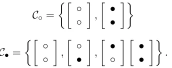
Scheme RG1. Scheme RG1 constructs the first share as a uniform random grid and the second share by assigning to pixel (i, j) the same color of the pixel (i, j) in the first share, if the secret pixel (i, j) is white, and the “opposite” color if the secret pixel (i, j) is black. The representation with distribution matrices of RG1, that is, the equivalent scheme in the probabilistic model, is described by the following collections:
C◦=
◦ ◦
,
• •
C•=
◦ •
,
• ◦
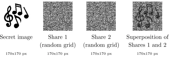
Secret image Share 1 Share 2 Superposition of (random grid) (random grid) Shares 1 and 2
170x170 px 170x170 px 170x170 px 170x170 px
Figure 1: Example of shares and superposition for scheme RG1.
Figure 1 shows the shares, and the superposition of the two shares that reveals the secret image. The shares are uniform random grids, hence the average light transmission over each single share is 1/2. In the reconstructed imageR, the area that corresponds to black pixels of the secret imageI, that is BI(R), is reconstructed as a completely black area. Thus λ•(RG1) = 0. Hence, with RG1,
black pixels are reconstructed in a perfect way. Instead WI(R) consists of white and black pixels
uniformly distributed over the region WI(R), and thus λ◦(RG1) = 1/2. Hence, γrg= 0.5. If we see the scheme as a probabilistic scheme with m = 1, we have that pw|w = 1/2 and pb|b = 1 and thus
β = 0.5.
Scheme RG2. Scheme RG2 generates again the first share as a uniform random grid. The second share is equal to the first when the secret pixel is white but if the secret pixel is black then also the second share is chosen at random. Scheme RG2 is described by the following collections:
C◦=
◦ ◦
,
• •
C• =
◦ ◦
,
◦ •
,
• ◦
• •
.
Figure 2 shows the shares and the superposition. The shares are again uniform random grids. However this time we have λ◦(RG2) = 0.5 and λ•(RG2) = 0.25 and thus the contrast is γrg = (0.5−0.25)/1.25 = 0.2. The white area WI(R) is reconstructed as in the previous example, but the black area BI(R) is not reconstructed perfectly but with, in average, 3 black pixels out of four
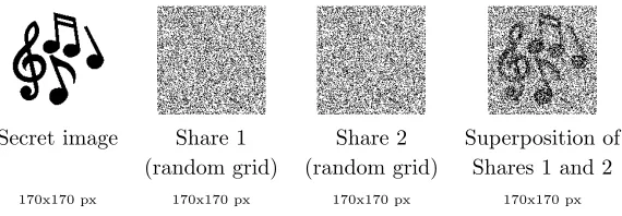
Secret image Share 1 Share 2 Superposition of (random grid) (random grid) Shares 1 and 2
170x170 px 170x170 px 170x170 px 170x170 px
Figure 2: Example of shares and superposition for scheme RG2.
with probability 3/4, that is pb|b = 3/4, and white with probability 1/4, that is pw|b = 1/4. Thus
pb|b−pb|w = 1/4.
Scheme RG3. In this scheme the first share is again generated at random while the second one is also generated at random if the secret pixel is white, and is the “opposite” of the first share if the secret pixel is black. Scheme RG3 is:
C◦ =
◦ ◦
,
◦ •
,
• ◦
,
• •
C• =
◦ •
,
• ◦
.
Secret image Share 1 Share 2 Superposition of (random grid) (random grid) Shares 1 and 2
170x170 px 170x170 px 170x170 px 170x170 px
Figure 3: Example of shares and superposition for scheme RG3.
Figure 3 shows the shares and the reconstruction. Again the shares are uniform random grids. This time we haveλ◦(RG3) = 0.25 andλ•(RG3) = 0 and thus the contrast isγrg = 0.25. The white area WI(R) is reconstructed with, in average, 3 black pixels out of four pixels while the black area
BI(R) is reconstructed perfectly. If we see the scheme as a probabilistic scheme withm= 1, we have that β= 0.25.
Scheme RG4. Finally we present another example of a random grid (2,2)-threshold scheme that uses generalized (non-uniform) random grids. Scheme RG4 is described by the following collections:
C◦=
◦ ◦
,
◦ ◦
,
• •
C• =
◦ ◦
,
◦ •
,
• ◦
Secret image Share 1 Share 2 Superposition of (random grid) (random grid) Shares 1 and 2
170x170 px 170x170 px 170x170 px 170x170 px
Figure 4: Example of shares and superposition for scheme RG4.
Figure 3 shows the shares and the reconstruction. This time the shares are not unifrom random grids but they are generalized random grids, since each single share has more white pixels (2/3) than black pixels (1/3). Although the shares have a non-uniform distribution of white and black pixels, each single share does not provide any information about the secret. The superposition of the shares produces a reconstructed imageR withλ◦(RG4) = 2/3 andλ•(RG4) = 1/3 and thus the contrast is
γrg= 1/4. The white areaWI(R) is reconstructed with, in average, 2 white pixels and 1 black pixel out of 3 pixels while the black areaBI(R) is reconstructed with 1 white pixel and 2 black pixels out of 3 pixels. If we see the scheme as a probabilistic scheme with m= 1, we have thatβ = 1/3.
3
Previous results
In this section we recall some known results that will be used later in the paper.
3.1 Deterministic VCS
In this section we recall some (relevant to this paper) results known for the deterministic visual cryptography model.
Theorem 3.1 [9, 19] In any deterministic (2, n)-threshold scheme we have that γns≤
dn/2ebn/2c n(n−1) .
We can construct (2, n)-threshold schemes that achieve optimalγnscontrast by using a black base matrix whose columns are all the binary vectors of weight bn/2cand a white base matrix consisting of nequal rows each with weight bn/n−2c−1 1
. The pixel expansion ism= bn/n2c
.
Theorem 3.2 [26] In any deterministic (n, n)-threshold scheme we have that γns ≤
1
2n−1 and m ≥ 2n−1.
We can construct (n, n)-threshold schemes that achieve optimalγnscontrast by using a black base matrix whose columns are all the binary vectors with an even weight (that is, µ•2i= 1 andµ•2i+1 = 0 fori= 0,1, . . .bn/2c) and a white base matrix whose columns are all the binary vectors with an odd weight (that is, µ◦2i = 0 andµ◦2i−1= 1 for i= 0,1, . . .dn/2e). The pixel expansion is m= 2n−1.
Bounds onγnsfor (3, n)-threshold schemes and (n−1, n)-threshold schemes are provided in Blundo et al. [7]. Krause and Simon [23] have provided a general (for any k) formula:
Theorem 3.3 [23] For any deterministic (k, n)-threshold scheme we have that
γns≤4
−(k−1) nk
A number of papers have considered the problem of finding schemes for which the reconstruction of black pixels is perfect, that is schemes for whichh=m. In particular we recall the following two constructions of (3, n)-threshold schemes.
Construction 3.4 [8] The white base matrix is described by µ◦0 = 1 and µ◦n−1 = n−2 (and the remaining µ◦s are equal to 0). The black base matrix is described by µ•n = (n−1)(2n−2) and µ•n−2 = 1 (and the remaining µ•s are equal to0).
Theorem 3.5 [8] Construction 3.4 yields deterministic (3, n)-threshold scheme withm = (n−1)2,
`=m−1 and h=m and thus γns=
1
n2−1.
Construction 3.6 [7] The white base matrix is described by
µ◦0=
n−1
bn+1 4 c
−
n−1
bn+1 4 c −1
, µ◦n−bn+1
4 c = 1
and all remaining µ•s are0. The white base matrix is described by
µ•n=
n−1
bn+1 4 c
−
n−1
bn+1 4 c −1
, µ◦bn+1
4 c = 1
and all remaining µ◦s are0.
Theorem 3.7 [7] Construction 3.6 (see Section 4.2 and Theorem 4.7 of [7]) yields a deterministic
(3, n)-threshold scheme with that m= 2 bn−n+11 4 c
andsγns=
(n−2)bn+1 4 cb
n+1 4 c
2(n−1)(n−2) .
Finally we recall the following construction of (n−1, n)-threshold schemes.
Construction 3.8 [8] The white base matrix is described by µ◦0 = 1 and µ2◦i+1 = 2i, for 1 ≤i ≤
(n−1)/2 (and the remaining µs are equal to 0). The black base matrix is described by µ•2i = 1, for 1≤i≤n/2 (and the remaining µs are equal to 0).
Theorem 3.9 [8] Construction 3.8 yields deterministic(n−1, n)-threshold schemes withm= (n−
2)2n−2+ 1, `=m−1 andh=m, and thus γns=
1 (n−2)2n−2+1. 3.2 Random Grid VCS
In this section we recall some (relevant to this paper) results for the random grid model. The following result has been proved by Shyu [28].
Construction 3.10 [28] There exists random grid (n, n)-threshold schemes with λ• = 0 and λ◦ =
1
2n−1 (thus withγrg=
1 2n−1).
The following has been proved by Chen and Lin [10].
Construction 3.11 [10] There exists random grid (2, n)-threshold schemes with contrast γrg =
c/n−(c/n)2
1+(c/n)2−1/n(1+c/n), where c∈ {bn(
√
Moreover in [10] it is proved (Theorem 4 of [10]) that the schemes of Construction 3.11 are such that
γrg ≤ 3−2√2
−2+2√2−1/n. Notice that this bound applies only to the schemes that have a particular form
(the one used by Construction 3.11).
Moreover [10] provides an extension of the (2, n)-threshold schemes yielding a (2,∞)-threshold scheme with γrg = (
√
2−1)/2 ' 0.2071. Among the schemes with the same form of Construc-tion 3.11, the (2,∞)-threshold scheme is asymptotically optimal because
lim
n→∞
3−2√2
−2 + 2√2−1/n = ( √
2−1)/2.
Chen and Tsao [12] provide constructions of random grid (k, n)-threshold schemes whose contrast is given in the next theorem.
Construction 3.12 [12] There exists (k, n)-threshold random grid schemes with contrast3
γrg= 2
(2k+ 1) n k
−1.
4
The connection between the random grid and the deterministic
model
In this section we present the main results of this paper. We prove that there is a strong connection between the random grid model and the deterministic model: for every random grid scheme there exists a corresponding deterministic scheme with similar characteristics and viceversa. This allows us to use results known in a model in the other model. As we have already pointed out it would have been possible to cast the same result by stating that the random grid model is equivalent to the probabilistic model with no pixel expansion. We have explained in Section 2.3 why we preferred not to pass through the probabilistic model.
Theorem 4.1 Every random grid scheme S with average light transmissions parameters λ◦ and
λ• and cardinality parameters m◦ and m•, can be transformed into a deterministic scheme S0 with
m=LCM(m◦, m•), `=m(1−λ◦) and h=m(1−λ•).
Proof: By Fact 2.4 we have that scheme S can be described by two distribution collections C◦ and
C•. Let m◦ and m• be the cardinality parameters of S. Construct scheme S0 with the following
base matrices. Letmbe the least common multiple LCM(m◦, m•) ofm◦ andm•. Base matrixB◦ is
obtained by concatenatingm/m• copies of each of the vectors inC◦ while base matrixB• is obtained
by concatenatingm/m◦ copies of each of the vectors inC•.
Since S0 is obtained by concatenating matrices ofS, the security property of S0 derives directly from the security property ofS. Moreover, by the definition ofλ◦and λ• we have that`=m(1−λ◦)
and h=m(1−λ•).
3
In [12] it is proved that when superposingt≥k shares the contrast isγrg = 2·(t
k) (2t+1)(n
k)−( t k)
.We have to consider
Theorem 4.2 Every deterministic scheme S with pixel expansion mand contrast parameters `and
h, can be transformed into a random grid scheme S0 with average light transmission parameters
λ◦= 1− m` andλ•= 1−mh.
Proof: Let C◦ and C• be the distribution collections of S. Construct C◦0 from C◦ by taking all the
columns that appear in any of the matrices of C◦. Notice that C◦0 is a multiset if there are repeated
columns. Similarly constructC0
• from C•. SchemeS0 is the random grid scheme described by C◦0 and
C•0 (see Fact 2.3).
Let Q be a forbidden set of participants. Then by the security property of S we have that the sets D◦ = {M|X, for each M ∈ C◦} and D• = {M|X, for each M ∈ C•} are indistinguishable in
the sense that they contain the same matrices with the same frequencies. This implies that the sets
D0◦ ={M|X, for each M ∈ C◦0} and D0• = {M|X, for each M ∈ C•0} are equal. Hence we have that
λ◦(Q) =λ•(Q).
Let Q be a qualified set of participants. Then by the contrast property, for any M ∈ C◦, we
have thatw•(sup(M|Q))≤`and for anyM ∈ C•, we have thatw•(sup(M|X))≥h. SinceC◦0 (resp.
C0
•) has been obtained by simply concatenating (a number of copies of) the matrices M ∈ C◦ (resp.
M ∈ C•) we have thatλ◦(Q)≤(m−m`)/m(resp. h≥(m−mh)/m). Hence we can setλ◦ = 1−m`
and λ•= 1−mh for schemeS0.
What Theorems 4.1 and 4.2 say is that there is a strong correspondence between the random grid model and the deterministic model.
Given a random grid scheme S and a deterministic scheme S0 related by Theorem 4.1 (or by
Theorem 4.2, swapping the names), we have that
γes(S
0
) = h−` 2m−h =
m(1−λ•)−m(1−λ◦)
2m−m(1−λ•)
= λ◦−λ• 1 +λ•
=γrg(S) (6)
and
γns(S
0
) = h−`
m =
m(1−λ•)−m(1−λ◦)
m =λ◦−λ•. (7)
Theorems 4.1 and 4.2 allow us to prove also the following results.
Theorem 4.3 Let f(n) be an upper bound on γns in the deterministic model (resp. random grid model). Then we have that f(n) is un upper bound on γns also in the random grid model (resp. deterministic model).
Proof: Assume that f(n) is an upper bound on γns in the deterministic model and assume by contradiction that the theorem does not hold and thus that there exists a random grid scheme
S with γns(S) > f(n). Then by Theorem 4.1 we can construct a deterministic scheme S
0 with
γns(S
0) = γ
ns(S) > f(n). This contradicts the fact that f(n) is an upper bound on γns in the deterministic model.
Similarly, assume that f(n) is an upper bound on γns in the random grid model. The proof is as before swapping “random model” with “deterministic” and using Theorem 4.2 instead of Theo-rem 4.1.
Proof: Assume that f(n) is an upper bound on γes in the deterministic model and assume by contradiction that the theorem does not hold and thus that there exists a random grid scheme
S with γrg(S) > f(n). Then by Theorem 4.1 we can construct a deterministic scheme S
0 with
γes(S
0) = γ
rg(S) > f(n). This contradicts the fact that f(n) is an upper bound on γes in the deterministic model.
Similarly, assume thatf(n) is an upper bound onγrg in the random grid model. The proof is as before swapping “random model” with “deterministic”, swappingeswithrgand using Theorem 4.2
instead of Theorem 4.1.
Notice that, by the definitions, we have that γes ≤ γns hence an upper bound on γns is also an upper bound onγes(and onγrg, sinceγrg=γes). This observation can be used to prove the following theorem.
Theorem 4.5 Let f(n) be an upper bound onγns in the deterministic model then we have that f(n) is un upper bound on γrg also in the random grid model.
Proof: Assume that f(n) is an upper bound on γns in the deterministic model and assume by contradiction that the theorem does not hold and thus that there exists a random grid scheme
S with γrg(S) > f(n). Then by Theorem 4.1 we can construct a deterministic scheme S
0 with
γes(S
0) = γ
rg(S) > f(n). Since γes(S
0) ≤γ
ns(S
0) we have thatγ
ns(S
0) > f(n). This contradicts the
fact that f(n) is an upper bound onγns in the deterministic model.
5
Threshold schemes
In this section we focus the attention on (k, n)-threshold schemes and provide new results in the random grid model (resp. in the deterministic model) starting from known results in the deterministic model (resp. random grid model).
5.1 (2, n)-threshold schemes
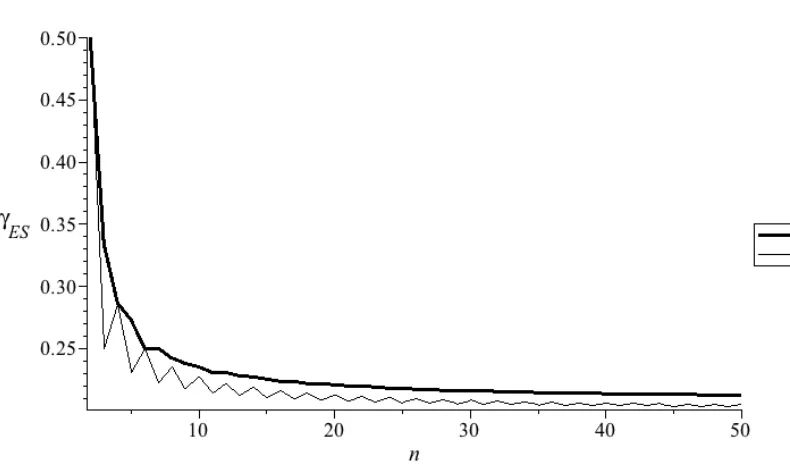
Theorem 5.1 For any random grid (2, n)-threshold schemeS we have that γrg(S)≤
dn/2ebn/2c n(n−1) .
Proof: Immediate consequence of Theorems 3.1 and 4.5.
Notice that the bound of Theorem 5.1 is general while the bound of Chen and Lin (see paragraph after Construction 3.11), applies only to a particular classs of schemes.
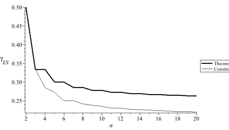
Figure 5: Upper bound onγrg(thick line) and value of contrast of schemes of Costruction 3.11 (thin line).
5.1.1 Schemes.
We can exploit the random grid (2, n)-threshold schemes of [10] to obtain new deterministic schemes that improve the contrastγes. First we give a construction very similar to that of [10].
Construction 5.2 Letc∈ {bn(√2−1)c,dn(√2−1)e}. A random grid share for a black secret pixel is chosen at random in the set of all possible nc vectors having c elements equal to ◦ and n−c
elements equal to•. Instead, a random grid share for a white secret pixel is chosen at random in the multiset of vectors consisting of n−c−11
vectors with all elements equal to ◦ and nc
− n−c−11
vectors with all elements equal to•. Among the two possible values forc, choose the one that maximizes γes.
Notice that this construction is slightly different from that of [10]. Our construction ensures that the cardinality parameters are equal, that is m◦ = m•. This helps in constructing deterministic
schemes with a smaller pixel expansion.
Example. Let us consider an example. For n= 5 we have thatc= 2 and
C• =
C◦= ◦ ◦ ◦ ◦ ◦ , ◦ ◦ ◦ ◦ ◦ , ◦ ◦ ◦ ◦ ◦ , ◦ ◦ ◦ ◦ ◦ , • • • • • , • • • • • , • • • • • , • • • • • , • • • • • , • • • • • .
Construction 5.2 (see Theorem 1 of [10]) gives a random grid (2, n)-threshold scheme and (by the proof of Theorem 2 in [10]) we have that the parameters areλ◦=c/nand λ•= ncn−c−11.
By Theorem 4.1, starting from schemes obtained with Construction 5.2, we can construct deter-ministic schemes, that we denote with An. We have that for scheme An
m= n c ,
`=m
1− c n
,
and
h=m
1− c(c−1) n(n−1)
.
Hence we have
γes(An) =
h−`
2m−h =
c n
1− c−1
n−1
1 +ncn−c−11
In the deterministic model optimal contrast schemes have been studied only with respect toγns. Thus the best comparison we can make is with the schemes that are optimal with respect toγns (see Theorem 3.1 and the subsequent paragraph). Denote with Bn such schemes. Obviously we have to
compare the contrastγes=γrg of such schemes. For schemesBnwe have:
m=
n bn/2c
,
`=
n−1
bn/2c −1
, and h= n bn/2c
−
n−2
bn/2c
.
Hence we have
γes(Bn) =
h−`
2m−h =
n−1
bn/2c
− bn/n2c
n bn/2c
+ bn/n−22c.
Figure 6: Comparison of the contrast γes(An) (thick line) withγes(Bn) (thin line).
5.2 (3, n)-threshold schemes
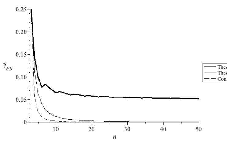
We provide two constructions for new random grid schemes based on two different deterministic (3, n)-threshold schemes. The first construction allows an easy analytical comparison with previous random grid schemes. The comparison shows that the new schemes have a better contrast. The second construction gives better schemes but the analytical comparison becomes more complicated. We provide empirical evidence that this second construction provides an improved contrast.
Theorem 5.3 The random grid(3, n)-threshold schemes obtained by using Construction 3.4 and the transformation of Theorem 4.2 has contrast
γrg= 1 (n−1)2.
Proof: By Theorem 3.5 we have that Construction 3.4 gives a deterministic (3, n)-threshold scheme with m= (n−1)2,h =m and `=m−1. By Theorem 4.2 we can transform such a scheme into a random grid scheme withλ◦= (n−11)2 and λ• = 0.
The contrast provided by the schemes of Theorem 5.3 is better than the contrast of the schemes of Construction 3.12. Indeed the (3, n)-threshold scheme of Chen and Tsao [12] have contrast
2 (23+1)(n
3)−1
. A simple algebra shows that (n−11)2 is always bigger than (23+1)2(n 3)−1
forn≥3. Indeed the condition (n−11)2 > (23+1)2(n
3)−1
is equivalent to 3n3−10n2+ 8n−3>0, which is true for n≥3.
Theorem 5.4 The random grid (3, n)-threshold scheme obtained using Construction 3.6 and Theo-rem 4.2 has contrast
γrg =
(n−1)(n−2)(n−2α)−(n−α)(n−α−1)(n−α−2) +α(α−1)(α−2) 2(n−1)(n−2)(n−α) + (n−α)(n−α−1)(n−α−2)
where α=bn+1 4 c.
Proof:By Theorem 3.7 we have that Construction 3.6 yields a deterministic (3, n)-threshold scheme withm= 2 bn−n+11
4 c
andγns=
(n−2)bn+1 4 cb
n+1 4 c
2(n−1)(n−2) . Unfortunately, Theorem 3.7 does not explicitly provide
the value of` andh.
In order to evaluate γrg we need to find` and h. LetQ be a qualified set of three participants. Parameter ` (resp. h), that is the number of black pixels in sup(B◦|Q) (resp. sup(B•|Q)) is given
by m minus the number of the 3-white-pixel columns inB◦|Q(resp. B•|Q).
To find ` notice that in B◦ we have µ◦0 all-white columns and thus these columns will count
for µ◦0 3-white-pixel columns in B◦|Q. In the remaining part of B◦ we have all the columns with
exactlyn− bn+14 cblack pixels. Hence among these columns inB◦|Q, there will be exactly n−bn−n+13 4 c
3-white-pixel columns. Since ` is equal to m minus the number of 3-white-pixel columns, we have that `=m−µ◦0− n−bn−n3+1
4 c
.
To findh notice that inB• we haveµ•n all-black columns and thus among these columns inB•|Q
there will be no 3-white-pixel columns. In the remaining m−µ•n columns of B• we have all the
columns with exactlybn+14 cblack pixels. Hence among these columns in B•|Q, there will be exactly n−3
bn+1 4 c
3-white-pixel columns. Since h is equal tom minus the number of 3-white-pixel columns of
B◦|Q, we have thath=m− bn−n+13 4 c
.
Now we have`,h andmso we can assessγrg = 2h−`m−h and, recalling thatµ◦0= bn−n+11 4 c
− bnn−+11 4 c−1
we get
γrg=
n−1
bn+14 c
− bnn−+11 4 c−1
− bn−n+13 4 c
+ n−bn−n3+1 4 c
2 bn−n+11 4 c
+ bn−n+13 4 c
.
To provide a closed form for the above expression, let us recall some well-known equalities involving binomial coefficients. The simmetry relation
a b
=
a a−b
, (8)
the addition formula
a b
=
a−1
b−1
a−1
b
, (9)
the equalities
a b
= a
b
a−1
b−1
, (10)
and
a c
a−c
b
=
a b
a−b
c
From (9) used witha=n,b=bn+1
4 c, we have that
n−1
bn+14 c
−
n−1
bn+14 c −1
= n−2b
n+1 4 c
n
n bn+14 c
(12)
From (11) used witha=n,b=bn+14 c and c= 1, we have that
n−1
bn+1 4 c
= n− b
n+1 4 c
n
n bn+1
4 c
(13)
Again from (11) used with a=n,b=bn+1
4 cand c= 3, we have that
n−3
bn+14 c
= (n− b
n+1
4 c)(n− b
n+1
4 c −1)(n− b
n+1 4 c −2)
n(n−1)(n−2)
n bn+14 c
(14)
From (8) used witha=n−3, b=n− bn+14 c we have that
n−3
n− bn+14 c
=
n−3
bn+14 c −3
while using three times (10) we have that
n bn+14 c
= n(n−1)(n−2)
bn+14 c(bn+14 c −1)(bn+14 c −2)
n−3
bn+14 c −3
.
Combining the previous two equalities we get
n−3
n− bn+1 4 c
= b
n+1 4 c(b
n+1
4 c −1)(b
n+1 4 c −2)
n(n−1)(n−2)
n bn+1
4 c
(15)
Using Equations(12)-(15), with a few algebraic transformations and cancelling out the common term
n bn+14 c
, we have that
γrg=
n−2bn+1 4 c
n −
(n−bn+1 4 c)(n−b
n+1
4 c−1)(n−b n+1
4 c−2)
n(n−1)(n−2) +
bn+1 4 c(b
n+1 4 c−1)(b
n+1 4 c−2)
n(n−1)(n−2)
2n−b n+1
4 c
n +
(n−bn+14 c)(n−bn+14 c−1)(n−bn+14 c−2)
n(n−1)(n−2)
(16)
from which the theorem follows by taking the least common multiple both for the numerator and the denominator and cancelling it out.
Corollary 5.5 The random grid (3, n)-threshold scheme obtained using Construction 3.6 and The-orem 4.2 has contrast
γrg=
2(n2−1)
41n2−138n+109 if n= 3 mod 4
2(n+2)
41n−38 if n= 2 mod 4
2(n+1)
41n−85 if n= 1 mod 4
2n2
Proof: By Theorem 5.4 we have that
γrg =
(n−1)(n−2)(n−2α)−(n−α)(n−α−1)(n−α−2) +α(α−1)(α−2) 2(n−1)(n−2)(n−α) + (n−α)(n−α−1)(n−α−2)
where α=bn+1
4 c. Observing that forn= 3 mod 4 we haveα=
n+1
4 , that for n= 2 mod 4 we have
α = n−42, that for n= 1 mod 4 we have α = n−41, and that forn= 0 mod 4 we have α= n4, it will be enough to substitute the appropriate value in the above formula for γrg, and after some tedious but simple algebraic transformations we get the corollary.
From the above corollary it is evident that for n→ ∞the value ofγrg approaches 2/41.
Example. Next we provide an example that will clarify the construction of the random grid schemes of Theorem 5.4. Let n = 4. Construction 3.6 gives the scheme where the non-zero µ’s are µ◦0 = 2, µ◦3= 1, µ•1 = 1, µ•4= 2. Hence the base matrices are:
B◦ =
◦◦•••◦ ◦◦••◦• ◦◦•◦•• ◦◦◦•••
B• =
•••◦◦◦ ••◦•◦◦ ••◦◦•◦ ••◦◦◦•
By using Theorem 4.2 we can transform such a scheme into a random grid scheme which is given by
C◦ =
◦ ◦ ◦ ◦ , ◦ ◦ ◦ ◦ , • • • ◦ , • • ◦ • , • ◦ • • ◦ • • •
C• =
• • • • , • • • • , • ◦ ◦ ◦ , ◦ • ◦ ◦ , ◦ ◦ • • ◦ ◦ ◦ • .
The contrast provided by the schemes of Theorem 5.4 improves on that of the schems of The-orem 5.3. Figure 5.2 shows empirical evidence. The figure includes also the contrast of schemes of Construction 3.12.
5.3 (n−1, n)-threshold schemes
Theorem 5.6 The random grid(n−1, n)-threshold schemes obtained by using Construction 3.8 and the transformation of Theorem 4.2 has contrast γrg=
1 (n−2)2n−2+1.
Figure 7: Comparison of the contrast for (3, n) schemes.
The contrast provided by the schemes of Theorem 5.6 is better than the contrast of schemes of Construction 3.12. Indeed the (n−1, n)-threshold scheme of Chen and Tsao [12] have contrast
2 (2n−1+1)( n
n−1)−1
. If we compute the difference we can easily see that it is always positive. Indeed
1
(n−2)2n−2+ 1−
2 (2n−1+ 1) n
n−1
−1 >0
is equivalent to
(2n−1+ 1)
n n−1
−1−2((n−2)2n−2+ 1)>0
and a simple algebra shows that the above is true for all n≥2.
5.4 (n, n)-threshold scheme
In this section we focus the attention on (n, n)-threshold schemes.
Theorem 5.7 For any random grid (n, n)-threshold scheme S we have that γrg(S)≤1/2
n−1.
Proof: Immediate consequence of Theorems 3.2 and 4.5.
The bound of Theorem 5.7 matches the contrast of the random grid (n, n)-threshold schemes of Shyu [28], hence:
The optimal (n, n)-threshold schemes by Shyu are the same as the ones we can get starting from the deterministic (n, n)-threshold schemes of Naor and Shamir.
Roughly speaking, the construction of Shyu [28] is as follows: the firstn−1 shares S1, . . . , Sn−1
are generated as independent random grids. The last shareSnis a function ofS1, . . . , Sn−1. Although
cast with a different formalism, this function sets the pixel of the last share in such a way that the total number of black pixels in the n shares is even if the secret bit is white and odd if the secret pixel is black. Hence Shyu’s random grid (n, n)-threshold scheme is in fact the same as the random grid (n, n)-threshold scheme that can be obtained by taking as possible distribution vectors all the vectors of the base matrices of the Naor and Shamir’s (n, n)-threshold scheme.
Example. Consider the casen= 3. The base matrices of Naor and Shamir (3,3)-threshold schemes are.
B◦=
◦◦•• ◦•◦• ◦••◦
B• =
•◦◦• ◦•◦• ◦◦••
The corresponding random grid (3,3) scheme is
C◦ =
◦ ◦ ◦
,
◦ • •
,
• ◦ •
,
• • ◦
C• =
• ◦ ◦
,
◦ • ◦
,
◦ ◦ •
,
• • •
.
The above scheme is the same one that is constructed by the construction of Shyu [28].
5.5 (k, n)-threshold schemes
Finally we give an upper bound onγrg valid for any value ofk.
Theorem 5.9 For any random grid (k, n)-threshold scheme we have that
γrg ≤4
−(k−1) nk
n(n−1)· · ·(n−(k−1)).
Proof: Immediate consequence of Theorems 3.3 and 4.5.
We have already considered upper bounds for the cases k = 2, n (Theorems 5.1 and 5.7). The general form provided above does not improve on the specific cases k = 2 and k = n. However it gives bounds for the other values of kfor which no bounds onγrg were known.
6
General Access Structure
shows a general technique that can be used to construct deterministic schemes for non-connected access structures. The same technique can be applied to random grid schemes.
Let A1 = (Q1,F1) and A2 = (Q2,F2) be two access structures on disjoint sets of participants.
Let A= (Q,F) be thesumof A1 andA2, given by
Q=Q1∪ Q2
and
F ={X∪Y|X∈ F1, Y ∈ F2}.
Given a scheme S1 = {C1
◦,C•1} for A1 and a scheme S2 = {C◦2,C•2} for A2, Theorem 5.5 of [2]
shows that there exists a scheme S ={C◦,C•} with access structure A. The scheme is obtained by
letting
C◦ =
M0 M00
:M0 ∈ C◦1, M00∈ C◦2
and
C• =
M0 M00
:M0 ∈ C•1, M00∈ C•2
.
For the construction of Theorem 5.5 of [2] it is shown that one can assume, without loss of generality, that both scheme S1 and S2, have cardinality parameters that are equal, that is for each
Si, |C◦i| = |C◦i|. Although this assumption is without loss of generality, because we can replicate
matrices in each collection in order to have distribution collections of the same size, it increases the total number of matrices to consider and consequently the amount of randomness needed. It is not hard to see that the construction works even if we relax this requirement.
To clarify the technique let us see an example. Consider the (2,2)-threshold random grid scheme
S1 =RG1:
C◦=
◦ ◦
,
• •
C•=
◦ •
,
• ◦
and the (2,3)-threshold random grid scheme S2 given by the following collections
C◦=
◦ ◦ ◦
,
◦ ◦ ◦
,
• • •
C•=
• ◦ ◦
,
◦ • ◦
,
◦ ◦ •
.
The random grid scheme for A, with qualified sets
Q={{1,2},{3,4},{3,5},{4,5}},
C◦ = ◦ ◦ ◦ ◦ ◦ , ◦ ◦ ◦ ◦ ◦ , ◦ ◦ • • • , • • ◦ ◦ ◦ , • • ◦ ◦ ◦ , • • • • •
C• =
◦ • • ◦ ◦ , ◦ • ◦ • ◦ , ◦ • ◦ ◦ • , • ◦ • ◦ ◦ , • ◦ ◦ • ◦ , • ◦ ◦ ◦ • .
7
Conclusions
In this paper we have shown that random grid visual cryptography is strictly related to deterministic visual cryptography. As a consequence many results known for the deterministic model can be used in the random grid model and viceversa. In the current literature papers that deal with random grid ignore results known for the deterministic model and viceversa. A consequence of the results of this paper is that future work on visual cryptography in the random grid model should be compared to known results for the deterministic model and viceversa.
Although the connection established in this paper allows to re-use many known results, it also opens up new directions. For example, given the fact that the measure of contrast γrg used in the random grid model corresponds to the measure of contrast γes given in [18] for the deterministic model, it becomes interesting to further study γes in the deterministic model. Almost all the papers that studied the contrast in the deterministic model have used the definition of contrast γns given in [26] and little is known forγes.
Many problems remain open. For example it is possible to find better random grid (k, n)-threshold schemes? For k=nwe have proved that the known random grid schemes are optimal with respect to γrg. However for the other cases there is still a gap between the contrast of known schemes and the upper bound. For the case of k = 2, the schemes match the upper bound only for n = 2,3. Clearly the same question can be recast in the deterministic model: which is the optimal contrast
γes? Which are the optimal, with respect toγes, schemes?
Given the connection established in this paper, it will be enough to solve any of these open problems either in the random grid model with respect to γrg, or in the deterministic model with respect toγes.
References
[1] Adhikari A., and Sikdar S., A new (2,n)-visual threshold scheme for color images. In Proceedings of Indocrypt 2003, LNCS 2904, pp. 148–161, 2005.
[2] Ateniese G., Blundo C., De Santis A. and Stinson D. R. (1996) Visual cryptography for general access structures. Information and Computation, 129, pp. 86–106.
[4] Ateniese G., Blundo C., De Santis A. and Stinson D. R. Extended schemes for visual cryptography.
Theoretical Computer Science, vol. 250, pp. 143–161, 2001.
[5] Blundo C., Cimato S. and De Santis A. Visual cryptography schemes with optimal pixel expansion.
Theoretical Computer Science, vol. 369, pp. 169-182, 2006.
[6] Blundo C., De Bonis A. and De Santis A.. Improved schemes for Visual Cryptography.Designs, Codes and Cryptography, vol. 24, pp. 255-278, 2001.
[7] Blundo C., D’Arco P., De Santis A. and Stinson D. R. Contrast optimal threshold visual cryptography schemes.SIAM J. on Discrete Mathematics, vol. 16, pp. 224–261, 2003.
[8] Blundo C. and De Santis A. Visual cryptography schemes with perfect reconstruction of black pixels.
Journal for Computers & Graphics, vol. 22, pp. 449–455, 1998.
[9] Blundo C., De Santis A. and Stinson D. R. On the contrast in visual cryptography schemes.Journal of Cryptology, vol. 12, pp. 261–289, 1999.
[10] Chen S.-K., Lin S.-J. Optimal (2, n) and (2,∞) visual secret sharing by generalized random grids.
Journal of Visual Comm. and Image Repr., vol. 23, pp 677-684, 2012.
[11] Chen T.-H., Tsao K.-H. Visual secret sharing revisited. Pattern Recognition, vol. 42, pp. 2203–2217, 2009.
[12] Chen T.-H., Tsao K.-H. Threshold visual secret sharing by random grids.The Journal of Systems and Software, vol. 84, pp. 1197-1208, 2011.
[13] Cimato S., De Prisco R. and De Santis A., Colored visual cryptography without color darkening. Theo-retical Computer Science, Vol. 374(1-3), pp. 261-276, 2007.
[14] Cimato S., De Prisco R. and De Santis A. Optimal colored threshold visual cryptography schemes.
Designs, Codes and Cryptography, vol. 35, pp. 311–335, 2005.
[15] Cimato S., De Prisco R. and De Santis A. Probabilistic Visual Cryptography Schemes.Comput. J., vol. 49(1), pp. 97–107, 2006.
[16] Visual Cryptography and Secret Image Sharing, Cimato S. and Yang C.-N. editors, CRC Press, Boca Raton, Florida, USA, ISBN 978-1-4398-3721-4, 2012.
[17] De Prisco R. and De Santis A., Using Colors to Improve Visual Cryptography for Black and White Images, Proceedings of ICITS 2011, LNCS 6673, pp. 182–201, 2011.
[18] Eisen P.A. and Stinson D.R., Threshold Visual Cryptography Schemes with Specified Whiteness Levels of Reconstructed Pixels.Designs, Cods and Cryptography, vol. 25, pp. 15–61, 2002.
[19] Hofmeister T., Krause M. and Simon H. U., Contrast-optimalkout ofnsecret sharing schemes in Visual Cryptography.Theoretical Computer Science, 240, pp. 471–485, 2000.
[20] Y.-C. Hou. Visual cryptography for color images.Pattern Recognition, vol. 36, pp. 1619–1629, 2003.
[21] Kafri O. and Keren E., Encryption of pictures and shapes by random grids. Optics Letters, vol. 12, n. 6, pp. 377-379, 1987.
[22] Koga H. and Yamamoto H., Proposal of a Lattice-Based Visual Secret Sharing Scheme for Color and Gray-Scale Images.IEICE Trans. on Fundamentals of Electronics, Communication and Computer Sci-ences, Vol 81-A(6), pp. 1262–1269, 1998.
[23] Krause M. and Simon H. U. Determining the optimal contrast for secret sharing schemes in visual cryptography.Combinatorics, Probability and Computing, vol. 12, pp. 285–299, 2003.
[25] Lu S., Manchala D. and Ostrovsky R.. Visual cryptography on graphs. J. Comb. Optim., vol 21, pp. 47–66, 2011.
[26] Naor M. and Shamir A. Visual cryptography. In Proceedings of Eurocrypt 94, LNCS 950, pp. 1–12, 1994.
[27] Shyu S.-J., Image encryption by random grids.Pattern Recognition, vol. 40, pp. 1014–1031, 2007.
[28] Shyu S.-J., Image encryption by multiple random grids. Pattern Recognition, vol. 42, pp. 1582–1596, 2009.
[29] Simon H.U., Perfect Reconstruction of Black Pixels Revisited. Proceedings of FCT 2005, LNCS 3623, pp. 221–232, 2005.
[30] Verheul E. R. and van Tilborg H. C. A. Constructions and properties ofkout ofnvisual secret sharing schemes.Designs, Codes, and Cryptography, vol. 11, pp. 179–196, 1997.
[31] Wang R.-Z., Lan Y.-C., Lee Y.-K., Huang, Shyu S.-J., Chia T.-L., Incrementing visual cryptography using random grids.Optics Communication, vol. 283, pp. 4242–4249, 2010.
[32] Yang C-N. New Visual Secret Sharing Schemes using Probabilistic Method.Pattern Recognition Letters, vol. 25, pp. 481–494, 2004.
[33] Yang C-N. and Chen T-S. Size-adjustable visual secret sharing schemes. IEICE Transactions on Fun-damentals of Electronics, Communications and Computer Sciences, vol. E88-A, pp. 2471–2474, 2005.
[34] Yang C-N. and Chen T-S. Aspect ratio invariant visual secret sharing schemes with minimum pixel expansion Pattern Recognition Letters, vol. 26, pp. 193–206, 2005.