All or Nothing at All
∗Paolo D’Arco1, Navid Nasr Esfahani2, and Douglas R. Stinson†2
1Dipartimento di Informatica, Universit`a degli Studi di Salerno, 84084 Fisciano (SA), Italy
2David R. Cheriton School of Computer Science, University of Waterloo, Waterloo, Ontario N2L 3G1, Canada
October 8, 2015
Abstract
We continue a study of unconditionally secure all-or-nothing transforms (AONT) begun in [12]. An AONT is a bijective mapping that constructs s outputs from s inputs. We consider the security oft inputs, when s−toutputs are known. Previous work concerned the caset= 1; here we consider the problem for generalt, focussing on the caset = 2. We investigate constructions of binary matrices for which the desired properties hold with the maximum probability. Upper bounds on these probabilities are obtained via a quadratic programming approach, while lower bounds can be obtained from combinatorial constructions based on symmetric BIBDs and cyclotomy. We also report some results on exhaustive searches and random constructions for small values ofs.
1
Introduction
Rivest defined all-or-nothing transforms in [10] in the setting of computational security. Stinson considered unconditionally secure all-or-nothing transforms in [12]. Here we extend some of the results in [12] by considering more general types of unconditionally secure all-or-nothing transforms.
Let X be a finite set, called an alphabet. Let s be a positive integer, and suppose that φ : Xs → Xs. We will think of φ as a function that maps an input s-tuple, say
x= (x1, . . . , xs), to an outputs-tuple, sayy= (y1, . . . , ys), where xi, yi ∈X for 1≤i≤s. Informally, the function φ is an unconditionally secure all-or-nothing transform provided that the following properties are satisfied:
1. φis a bijection.
∗
We have “borrowed” the title of this paper from the classic song of the same name written by Altman and Lawrence in 1939. It was recorded by Frank Sinatra and the Harry James Orchestra in 1939, and became a huge hit in 1943.
†
2. If anys−1 of thesoutput valuesy1, . . . , ysare fixed, then the value of any one input valuexi (1≤i≤s) is completely undetermined, in an information-theoretic sense.
We will denote such a function as an (s, v)-AONT, where v=|X|.
The above definition can be rephrased in terms of the entropy function, H, as follows. Let X1, . . . , Xs, Y1, . . . , Ys be random variables taking on values in the finite set X. (The variables X1, . . . , Xs need not be independent, or uniformly distributed.) Then these 2s random variables define an AONT provided that the following conditions are satisfied:
1. H(Y1, . . . , Ys|X1, . . . , Xs) = 0.
2. H(X1, . . . , Xs|Y1, . . . , Ys) = 0.
3. H(Xi | Y1, . . . , Yj−1, Yj+1, . . . , Ys) = H(Xi) for all i and j such that 1 ≤ i ≤ s and 1≤j≤s.
Rivest [10] defined AONT to provide a mode of operation for block ciphers that would require the decryption of all blocks of an encrypted message in order to determine any specific single block of plaintext. He called it the “package transform”. The method is very simple and elegant. Suppose we are given s blocks of plaintext, (x1, . . . , xs). First,
we apply an AONT, computing (y1, . . . , ys) =φ(x1, . . . , xs). Then we encrypt (y1, . . . , ys)
using a block cipher. At the receiver’s end, the ciphertext is decrypted, and then the inverse transformφ−1 is applied to restore the splaintext blocks. Note that the transformφis not secret. Extensions of this technique are studied in [1, 5].
All-or-nothing transforms have turned out to have numerous applications in cryptogra-phy and security. Here are some representative examples:
• exposure-resilient functions [2]
• network coding [3, 6]
• secure data transfer [14]
• anti-jamming techniques [9]
• secure distributed cloud storage [8, 11]
• query anonymization for location-based services [15].
We note that the above definition of an unconditionally secure AONT does not say anything regarding partial information that might be revealed about more than one of the
sinput values. For example, it does not rule out the possibility of determining the exclusive-or of two input values, given some relatively small number of output values. This motivates the following more general definition. Let 1≤t≤s. We will say thatφis at-all-or-nothing transform provided that the following properties are satisfied:
1. φis a bijection.
2. If anys−tof the s output valuesy1, . . . , ys are fixed, then anyt of the input values
We will denote such a function as a (t, s, v)-AONT, wherev=|X|. Note that the original definition corresponds to a 1-all-or-nothing transform.
This definition can also be rephrased in terms of the entropy function. As before, let
X1, . . . , Xs, Y1, . . . , Ys be random variables taking on values in the finite set X. These 2s random variables define a t-AONT provided that the following conditions are satisfied:
1. H(Y1, . . . , Ys|X1, . . . , Xs) = 0.
2. H(X1, . . . , Xs|Y1, . . . , Ys) = 0.
3. For all X ⊆ {X1, . . . , Xs} with |X |=t, and for all Y ⊆ {Y1, . . . , Ys} with |Y|=t, it holds that
H(X | {Y1, . . . , Ys} \ Y) =H(X). (1)
1.1 Organization of the Paper
The rest of this paper is organized as follows. In Section 2, we give our basic result that characterizes linear AONT in terms of matrices having invertible submatrices. We also give a construction using Cauchy matrices over a finite field Fq, which is applicable provided that q ≥ 2s. It turns out that it is impossible to construct linear AONT over F2, so an
interesting question is how “close” one can get to an AONT in this setting. In Section 3, we give some preliminary results and analyze one infinite class of matrices. In Section 4, we derive an upper bound on the maximum number of invertible 2 by 2 submatrices of an invertible s by s 0−1 matrix (this is relevant for the study of 2-AONT). We use a method based on quadratic programming to prove our bound. In Section 5, we discuss five construction methods for invertiblesby s0−1 matrices containing a large number of invertible 2 by 2 submatrices. The five methods are
1. exhaustive search,
2. a random construction,
3. a recursive construction,
4. a construction using symmetric balanced incomplete block designs (SBIBDs), and
5. a construction based on cyclotomy.
We achieve our best asymptotic results from SBIBDs, where we have an infinite class of examples that are close to the upper bound derived in the previous section. In Section 6, we turn to arbitrary (i.e., linear or nonlinear) AONT, and describe some connections with orthogonal arrays. Finally, Section 7 is a brief summary.
2
Linear AONT
We are mainly going to consider linear transforms. Let Fq be a finite field of orderq. An AONT with alphabet Fq is linear if each yi is an Fq-linear function of x1, . . . , xs. Then,
We will also be interested in functions that satisfy the condition (1) for certain (but not necessarily all) pairsX,Y. This will be particularly relevant in the case whereφis a binary linear transformation. More specifically, supposeq = 2r for some r ≥1 and M is defined over the subfieldF2(soMis a 0−1 matrix). This could be desirable from an efficiency point
of view, because the only operations required to compute the transform are exclusive-ors of bitstrings. However, it turns out that there are no nontrivial 1-AONT (a fact that was already observed in [12]). So it is a reasonable and interesting problem to study how close we can get to an AONT in this setting. We will give a precise answer to this question for
t= 1 in Theorem 3.5; much of the rest of this paper will study the corresponding problem whent= 2.
For I, J ⊆ {1, . . . , s}, define M(I, J) to be the |I| by |J| submatrix of M induced by thecolumnsinI and therowsinJ. The following lemma characterizes linear all-or-nothing transforms in terms of properties of the matrixM. This lemma can be considered to be a generalization of [12, Theorem 2.1].
Lemma 2.1. Suppose that q is a prime power and M is an invertible s by s matrix with entries from Fq. Let X ⊆ {X1, . . . , Xs}, |X |=t, and let Y ⊆ {Y1, . . . , Ys}, |Y|=t. Then
the functionφ(x) =xM−1 satisfies (1) with respect toX andY if and only if the submatrix
M(I, J) is invertible, where I ={i:Xi ∈ X }and J ={j:Yj ∈ Y}.
Proof. Let x0 = (xi :i∈I). We have x0 =yM(I,{1, . . . , s}). Now assume that yj is fixed for allj∈J. Then we can writex0 =y0M(I, J)+c, wherey0 = (yj :j ∈J) andcis a vector of constants. IfM(I, J) is invertible, thenx0 is completely undetermined, in the sense that
x0 takes on all values in (Fq)t asy0 varies over (Fq)t. On the other hand, if M(I, J) is not
invertible, thenx0 can take on only (Fq)t
0
possible values, whererank(M(I, J)) =t0 < t.
An s by sCauchy matrix can be defined over Fq if q ≥2s. Let a1, . . . , as, b1, . . . , bs be distinct elements ofFq. Letcij = 1/(ai−bj), for 1≤i≤sand 1≤j ≤s. Then C = (cij) is the Cauchy matrix defined by the sequence a1, . . . , as, b1, . . . , bs. The most important property of a Cauchy matrix C is that any square submatrix of C (including C itself) is invertible overFq.
Cauchy matrices were briefly mentioned in [12] as a possible method of constructing AONT. However, they are particularly relevant in light of the stronger definitions we are now investigating. To be specific, Cauchy matrices immediately yield the strongest possible all-or-nothing transforms, as stated in the following theorem.
Theorem 2.2. Suppose q is a prime power and q ≥2s. Then there is a linear transform that is simultaneously a(t, s, q)-AONT for all tsuch that 1≤t≤s.
3
Linear Transforms over
F
2Remark 3.1. In the remainder of the paper, when we discuss invertibility of a matrix, we mean invertibility over F2.
There is no Cauchy matrix over F2 if s > 1. In fact, it is easy to see that there is no
motivates trying to determine how close we can get to a (1, s,2)-AONT, or more generally, to a (t, s,2)-AONT, for a givent, 1≤t≤s.
For future reference, we record the 2 by 2 invertible 0−1 matrices.
Lemma 3.1. A2 by 2 0−1 matrix is invertible if and only if it is one of the following six matrices:
1 1
1 0
1 1
0 1
0 1
1 1
1 0
1 1
1 0
0 1
0 1
1 0
.
We first consider an example.
Example 3.1. Define a 3 by 3 matrix:
M =
1 1 1
1 0 1
1 1 0
.
It is clear that seven of the nine 1 by 1 submatrices of M are invertible (namely, the “1” entries). There are nine2by2submatrices ofM and seven of them are seen to be invertible, from Lemma 3.1. The only non-invertible 2 by 2 submatrices are M({1,3},{1,2}) and
M({1,2},{1,3}). Finally, M itself is invertible.
It seems natural to quantify the “closeness” ofM to an all-or-nothing transform by con-sidering the ratio of invertible square submatrices to the total number of square submatrices (of a given sizet). Therefore, for ansbysinvertible 0−1 matrix M and for 1≤t≤s, we define
Nt(M) = number of invertiblet byt submatrices of M
and
Rt(M) =
Nt(M) s t
2 .
We refer toRt(M) as the t-density of the matrixM. For 1≤t≤s, we also define
Rt(s) = max{Rt(M) :M is ansby sinvertible 0−1 matrix}.
Rt(s) denotes the maximum t-density of anys bysinvertible 0−1 matrix.
For the matrix M from Example 3.1, we haveR1(M) = 7/9 and R2(M) = 7/9.
Lemma 3.2. Suppose M is ans bys 0−1 matrix having at mosts−2 zero entries. Then
M is not invertible.
Proof. There must exist at least two columns ofM that do not contain a zero entry. These two columns are identical, so they are linearly dependent.
Lemma 3.3. Suppose M = Js−Is, where Is denotes the s by s identity matrix and Js
denotes the sby s matrix in which every entry is equal to one. Then M is invertible over
Proof. If sis even, then it is easy to check that M−1 =M. If sis odd, then observe that the sum of all the columns of M yields the zero-vector, so we have a dependence relation among the columns ofM.
Lemma 3.4. Suppose M is an sby s0−1 matrix having exactlys−1 zero entries. Then
M is invertible over F2 if and only if the zero entries occur in s−1 different rows and in
s−1 different columns.
Proof. First suppose that there are at least two zero entries in a specific column of M. Then there must exist at least two columns of M that do not contain a zero entry, andM
is not invertible, as in Lemma 3.2. A similar conclusion holds if there exist at least two zero entries in a specific row of M. Therefore we can restrict our attention to the case where the zero entries occur ins−1 different rows and in s−1 different columns. We will show thatM is invertible in this case.
By permuting rows and columns if necessary (which does not affect invertibility), we can assume thatM = (mij) has the form
M =
1 1 1 1 . . . 1 1 0 1 1 . . . 1 1 1 0 1 . . . 1
..
. ... ... ... . .. ... 1 1 1 1 . . . 0
. (2)
We will prove thatM is invertible by induction ons. Clearly we can uses= 1 as a base case. Now we assume s≥2 and we evaluate detM overF2 by using a cofactor expansion
along the first column. This yields
detM =
s
X
i=1
mi1×det(Mi1)
= s
X
i=1
det(Mi1),
whereMi1 is theminor formed by deleting rowiand column 1 ofM.
We consider two cases, depending on whethersis even or odd. First, suppose that sis odd. Here, det(M11) = 1 from Lemma 3.3, and det(Mi1) = 1 for 2≤i≤sby induction. It
follows that det(M) =smod 2 = 1.
Now lets be even. We have that det(M11) = 0 from Lemma 3.3, and det(Mi1) = 1 for
2 ≤ i ≤ s by induction. It follows that det(M) = (s−1) mod 2 = 1. By induction, the proof is complete.
The following result is an immediate corollary of Lemmas 3.2 and 3.4.
Theorem 3.5. For all s≥1, we have R1(s) = 1−ss−21.
Remark 3.2. It was shown in [12] that R1(s)≥1−1s when sis even. This was based on
using the matrix Js−Is as a transform. Theorem 3.5 is a slight improvement, and it holds
Example 3.2. Consider the 4 by 4 matrix given by (2):
M =
1 1 1 1
1 0 1 1
1 1 0 1
1 1 1 0
.
Here, we can verify using Lemmas 3.2, 3.3 and 3.4 thatR1(M) = 13/16,R2(M) = 24/36 =
2/3 and R3(M) = 9/16.
In fact, it is possible to compute all the valuesRt(M) for thesby smatrixM given in (2). There are st2 submatrices N of M of dimensions t by t. From the structure ofM, and from Lemmas 3.2, 3.3 and 3.4, we see that a t by t submatrix N is invertible if and only if one of the following conditions holds:
1. N containst−1 zero entries, or
2. tis even and N containstzero entries.
If we can count the number of submatrices of this form, then we can computeRt(M). But this is not hard to do.
Lemma 3.6. The s by s matrix M given in (2) has exactly st−−11(1 + (s−t+ 1)(s−t))
submatrices that contain exactly t−1 zero entries.
Lemma 3.7. Thesby smatrixM given in (2) has exactly s−t1 submatrices that contain exactlyt zero entries.
So we now obtain the following.
Theorem 3.8. Let M be thes by s matrix given in (2) and let 1≤t≤s−1. If t is odd, then
Nt(M) =
s−1
t−1
(1 + (s−t+ 1)(s−t)).
If t is even, then
Nt(M) =
s−1
t
+
s−1
t−1
(1 + (s−t+ 1)(s−t)).
Theorem 3.8 also provides (constructive) lower bounds on Rt(s) for all values of t≤s. We do not claim that these bounds are necessarily good asymptotic bounds, however. Even for t = 2, we get R2(M) → 0 as s → ∞, since st−−11
(1 + (s−t+ 1)(s−t)) ∈ Θ(s3) and s
t
2
4
Upper Bounds for
R
2(
s
)
We first establish an easy upper bound for R2(s). This bound follows from the following
lemma.
Lemma 4.1. Any2 by s 0−1 matrix contains at most s2/3invertible 2 by 2 submatrices.
Proof. LetN be any 2 by s0−1 matrix. Consider the 2 by 1 submatrices of N. Suppose
there area0 occurrences of
0 0
,a1 occurrences of
0 1
,a2 occurrences of
1 0
, and
a3 occurrences of
1 1
. Of course a0+a1+a2+a3 =s. From Lemma 3.1, the number of
invertible 2 by 2 submatrices inN is easily seen to bea1a2+a1a3+a2a3. This expression
is maximized when a0 = 0, a1 = a2 =a3 = s/3, yielding 3(s/3)2 =s2/3 invertible 2 by 2
submatrices.
Theorem 4.2. For any s≥2, it holds that
R2(s)≤
2s
3(s−1).
Proof. From Lemma 4.1, in any two rows of M there are at most s2/3 invertible 2 by 2 submatrices. Now, in the entire matrixM, there are s2
ways to choose two rows, and there
are s22 submatrices of order 2. This immediately yields
R2(s)≤
s
2
(s2/3) s
2
2 =
2s
3(s−1).
Example 4.1. When s= 3, we only get the trivial upper bound R2(3)≤1 from Theorem
4.2. Consider the matrix
M =
0 1 1
1 0 1
1 1 0
.
It is clear from the proof of Theorem 4.2 that all nine2by2submatrices ofM are invertible, andM is the only 3 by 3 matrix with this property. However,M is not itself invertible, so we can conclude that R2(3)≤8/9. Example 3.1 shows that R2(3)≥7/9.
In fact, we can show that R2(3) = 7/9. Suppose that R2(3) = 8/9. Let R2(M) = 8/9.
Then we can assume that the first two rows ofM contain three invertible2by2submatrices, the first and third rows of M contain three invertible 2 by 2 submatrices, and the last two rows ofM contain two invertible 2 by 2 submatrices. By permuting columns, the first two rows of M look like:
0 1 1
1 0 1
.
In order that the first and third rows contain three invertible 2 by 2 submatrices, the third row must be1 0 1 or 1 1 0. In the first case, the last two rows of M contain no invertible 2
by 2 submatrices, and in the second case, the last two rows of M contain three invertible 2
Example 4.2. When s= 4, we get R2(4)≤8/9 from Theorem 4.2. Consider the matrix
M = J4 −I4. M is invertible from Lemma 3.3. It is easy to check that 30 of the 2 by 2
submatrices of M are invertible. Therefore, R2(4)≥5/6.
We can in fact show that R2(4) = 5/6, as follows. Suppose R2(4) > 5/6. Then there
is a 4 by 4 0−1 matrix M having at least 31 invertible 2 by 2 submatrices. There are six pairs of rows in M, and 31 >6×5, so there is at least one pair of rows that contains six invertible 2 by 2 submatrices. But this contradicts Lemma 4.1, where it is shown that the maximum number of 2 by 2 submatrices in two given rows is at most 42/3 = 16/3<6.
We next present a generalization of Theorem 4.2 that leads to an improved upper bound onR2(s). The proof of Theorem 4.2 was based on upper-bounding the number of invertible
2 by 2 submatrices in any two rows of an sby smatrixM. Here we instead determine an upper bound on the number of invertible 2 by 2 submatrices in any four rows of M. (It turns out that considering three rows at a time yields the same bound as Theorem 4.2, so we skip directly to an analysis of four rows at a time.)
Label the non-zero vectors in {0,1}4 in lexicographic order as follows: b
0 = (0,0,0,0),
b1 = (0,0,0,1), b2 = (0,0,1,0), b3 = (0,0,1,1), . . ., b15 = (1,1,1,1). For 1 ≤ i, j ≤ 15,
definecij to be the number of invertible 2 by 2 submatrices in the 4 by 2 matrix bTi bTj
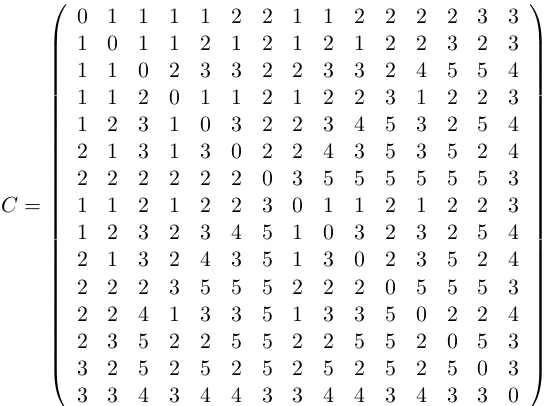
. Let C = (cij); note that C is a 15 by 15 symmetric matrix with zero diagonal such that every off-diagonal element is a positive integer. This matrixCis straightforward to compute and it is presented in Figure 1.
Now define z= (z1, . . . , z15) and consider the following quadratic program Q:
Maximize 12zCzT
subject to P15
i=1zi ≤1 and zi ≥0, for alli, 1≤i≤15.
We have the following result.
Theorem 4.3. For any integer s≥4, it holds that
R2(s)≤
γs
3(s−1),
where γ denotes the optimal solution to Q.
Proof. Let M be any s by s 0−1 matrix. Consider any four rows of M, say the first four rows without loss of generality, and denote the resulting 4 byssubmatrix byM0. For 0≤i≤15, suppose there areai columns ofM0 that are equal tobTi . The numberN of 2 by 2 invertible submatrices of M0 is equal to 12aCaT, where a = (a1, . . . , a15) (we can ignore
a0 because a zero column does not give rise to any invertible submatrices). If we now define
zi =ai/sfor all i, then we obtain
N = 1 2aCa
T = s2 2 zCz
T ≤γs2.
There are 4s
ways to choose four rows from M. The total number of occurrences of invertible 2 by 2 submatrices obtained is at most s4
C=
0 1 1 1 1 2 2 1 1 2 2 2 2 3 3
1 0 1 1 2 1 2 1 2 1 2 2 3 2 3
1 1 0 2 3 3 2 2 3 3 2 4 5 5 4
1 1 2 0 1 1 2 1 2 2 3 1 2 2 3
1 2 3 1 0 3 2 2 3 4 5 3 2 5 4
2 1 3 1 3 0 2 2 4 3 5 3 5 2 4
2 2 2 2 2 2 0 3 5 5 5 5 5 5 3
1 1 2 1 2 2 3 0 1 1 2 1 2 2 3
1 2 3 2 3 4 5 1 0 3 2 3 2 5 4
2 1 3 2 4 3 5 1 3 0 2 3 5 2 4
2 2 2 3 5 5 5 2 2 2 0 5 5 5 3
2 2 4 1 3 3 5 1 3 3 5 0 2 2 4
2 3 5 2 2 5 5 2 2 5 5 2 0 5 3
3 2 5 2 5 2 5 2 5 2 5 2 5 0 3
3 3 4 3 4 4 3 3 4 4 3 4 3 3 0
.
Figure 1: The objective function C for the quadratic program
submatrix is included in exactly s−22sets of four rows, so the total number of invertible 2 by 2 submatrices is at most
s
4
γs2
s−2 2
.
The total number of 2 by 2 submatrices is s22, so we obtain the upper bound
R2(s)≤
s
4
γs2
s−2 2
s
2
2 =
γs
3(s−1). (3)
In general, it can be difficult to find (global) optimal solutions for quadratic programs. We were able to solve our quadratic program Q using the BARON software [13] on the NEOS server (http://www.neos-server.org/neos/). The result is that γ = 15/8 and an optimal solution is given by z7 =z11 =z13 =z14 = 1/4, zi = 0 if i6∈ {7,11,13,14}. It is interesting to observe that this solution corresponds to the given set of four rows containing only columns consisting of three 1’s and one 0. In fact, when s = 4, this provides an alternative proof of Example 4.2.
Applying Theorem 4.3, we immediately obtain the following improved upper bound.
Corollary 4.4. For any s≥4, it holds that
R2(s)≤
5s
8(s−1).
It is of course possible to generalize this approach, by consideringρ rows at a time. The coefficient matrix C will have 2ρ−1 rows and columns. If γρ denotes the solution to the related quadratic program, then we obtain the following generalization of Theorem 4.3.
Theorem 4.5. For any integers s≥ρ≥2, it holds that
R2(s)≤
4γρ
ρ(ρ−1)×
s
s−1. (4)
Proof. The equation (3) becomes the following:
R2(s)≤
s ρ
γρs2
s−2
ρ−2
s
2
2 =
4γρ
ρ(ρ−1)×
s s−1.
The difficulty in obtaining improved bounds using this approach is that the optimal solutionsγρof the quadratic programs are hard to compute.
5
Constructions
In the next subsections, we consider five possible construction methods for AONT with good 2-density. The first is exhaustive search. The second is based on choosing each entry independently at random with an appropriate probability. The third technique is a recursive technique. The fourth method is based on using incidence matrices of symmetric BIBDs. Our fifth and last approach makes use of classical results concerning cyclotomy and cyclotomic numbers.
5.1 Exhaustive Searches
We used an exhaustive search in order to find an invertibles×smatrix with the maximum possible number of invertible 2×2 submatrices, for 4≤s≤8. The algorithm consists ofs
nested loops, each iterating over the possible values in a given row of the matrix. There are 2s possibilities for any given row. However, any permutation of rows and columns does not affect either the nonsingularity of the matrix or the number of invertible 2×2 submatrices. Therefore, the search algorithm only generated matrices in which each row has at least as many 1’s as the row immediately above it. Also, if two rows have the same number of 1’s, the row having the smaller representation as a binary number would appear higher. These two rules enabled us to search only a 1/s! fraction of the search domain. Finally, we partially restricted column permutations by fixing all the 1’s in the first row to occur in the rightmost positions. This also sped up the search process.
5.2 Random Constructions
We investigate the expected number of invertible 2 by 2 submatrices in a randomsbys0−1 matrixM. Suppose every entry of M is chosen to be a 1 with probability , independent of the values of all other entries. Using Lemma 3.1, it is easy to see that a specified 2 by 2 submatrix is invertible with probability
43(1−) + 22(1−)2 = 22(1−)(2+ 1−) = 22(1−2).
This function is maximized by choosing = p1/2. The expected number of invertible 2 by 2 submatrices in M is 12 s22
(leading to an expected 2-density of .5). Unfortunately, this does not immediately yield an AONT because it seems difficult to ensure that the constructed matrix is itself invertible. However, this random construction proves to be a useful method to obtain good small examples.
5.3 Recursive Constructions
We now investigate the possibility of constructing “good” AONT recursively. Specifically, we analyze a type of doubling construction in a particular case. We begin with the (2,4, 2)-AONT from Example 4.2. Recall that this 2)-AONT arises from the matrix J4 −I4 and it
achieves the optimal result R2(4) = 5/6. We might try to use this matrix to construct a
(2,8,2)-AONT. There are various ways in which we could try to do this; we present one method which leads to a reasonably good outcome. Consider the matrix
M =
J4−I4 J4−I4
J4−I4 J4
.
We first need to show thatM is invertible. We show that det(M) = 1 as follows. Consider a matrix of the form
M =
A B C D
,
where A, B, C, D are square submatrices and CD = DC. In this case, it is known that det(M) = det(AD−BC).
In our construction, we have CD = DC = 3J4 = J4, so this formula can be applied.
We haveA=B =C =J4−I4 and it is easy to check thatBC =I4,AD=J4. Therefore
AD−BC =J4−I4 and det(M) = det(AD−BC) = det(J4−I4) = 1.
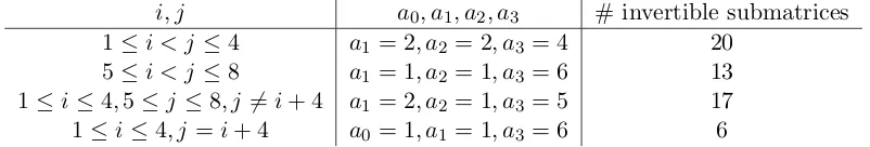
Next, we proceed to compute the number of 2 by 2 invertible submatrices of M. We do this by looking at pairs of rows ofM, say row iand rowj, and computing the relevant numbersa0, a1, a2, a3in each case (where we are using the notation from the proof of Lemma
4.1). We tabulate the results in Table 1.
The number of occurrences of the four cases enumerated in Table 1 is (respectively) 6,6,12 and 4. Therefore,
N2(M) = 6×20 + 6×13 + 12×17 + 4×6 = 426.
Finally, we compute
R2(M) =
426
8 2
2 =
426
784 =.5434.
Table 1: 2 by 2 invertible submatrices ofM
i, j a0, a1, a2, a3 # invertible submatrices
1≤i < j ≤4 a1 = 2, a2 = 2, a3 = 4 20
5≤i < j ≤8 a1 = 1, a2 = 1, a3 = 6 13
1≤i≤4,5≤j≤8, j=6 i+ 4 a1 = 2, a2 = 1, a3 = 5 17
1≤i≤4, j =i+ 4 a0 = 1, a1 = 1, a3 = 6 6
Theorem 5.1. N2(8)≥426 and R2(8)≥.5434.
It is interesting to note that this recursive construction yields a better result than the direct constructions considered previously. For example, if M =J8−I8, then we only get
thatN2 ≥364. Also, Theorem 3.8 (with s= 8, t= 2) only yieldsN2≥322.
5.4 Constructions from Symmetric BIBDs
We next give a construction which potentially achieves similar behaviour as the random construction, using symmetric balanced incomplete block designs (SBIBDs). A (v, k, λ) -balanced incomplete block design (BIBD) is a pair (X,A), whereX is a set ofv points and
A is a collection of k-subsets of X called blocks, such that every pair of points occurs in exactly λ blocks. Denote b = |A|; it is well-known that b = λv(v−1)/(k(k−1)). It is also the case that every point occurs in exactly r = bk/v = λ(v−1)/(k−1) blocks. A BIBD is symmetric if v = b. Equivalently, this condition can be expressed as r = k or
λ(v−1) =k(k−1).
Suppose (X,A) is a (v, k, λ)-BIBD. Denote X ={xi : 1≤ i≤ v} and A = {Aj : 1≤
j≤b}. Theincidence matrix of (X,A) is thevbyb0−1 matrixM = (mij) wheremij = 1 ifxi ∈Aj, and mij = 0 if xi6∈Aj.
Lemma 5.2. Suppose M is the incidence matrix of a symmetric (v, k, λ)-BIBD. Then M
is invertible overF2 if and only if k is odd and λis even.
Proof. It is well-known (see, e.g., [4]) that det(M) is an integer and
(det(M))2 =k2(k−λ)v−1.
Reducing modulo 2, we see that det(M)≡1 mod 2 if and only ifkis odd andλis even.
Theorem 5.3. Suppose M is the incidence matrix of a symmetric (v, k, λ)-BIBD where k
is odd andλ is even. Then
R2(M) =
k2−λ2
v
2
. (5)
Proof. First, sincek is odd andλis even,M is invertible overF2 by Lemma 5.2. Consider
two rows of M and define a0, a1, a2, a3 as in the proof of Theorem 4.2. Using the fact
that M is the incidence matrix of a symmetric (v, k, λ)-BIBD, it is not hard to see that
a0 =v−2k+λ,a1 =a2=k−λand a3 =λ. Then we can compute
From this, we haveN2(M) = v2
(k2−λ2) and (5) is easily derived.
Let’s try to figure out the best result that we could possibly obtain from Theorem 5.3. Suppose k ≈ cv. Then from the equation λ(v −1) = k(k−1), we see that λ ≈ c2v. Substituting into (5), we getR2(M)≈2(c2−c4). Now we of course have 0≤c≤1, and the
function 2(c2−c4) is maximized whenc=p1/2. In this case, we would get R2(M)≈1/2,
more-or-less matching the random construction from Section 5.2. We have also guaranteed that the matrixM is invertible. Of course, we would require a suitable SBIBD in order to get close to this bound.
We consider some examples to illustrate the application of Theorem 5.3.
Example 5.1. It is known [4] that there is a(31,21,14)-SBIBD. Noting that21is odd and
14 is even, the incidence matrix of this design is invertible overF2 by Lemma 5.2. Observe
that21/31 is quite close top1/2, so we expect a good result. Applying Theorem 5.3, we get
R2(M) =
212−142
31 2
=
49
93 ≈.5269.
Example 5.2. There also exists (40,27,18)-SBIBD (see [4]). Noting that 27is odd and18
is even, the incidence matrix of this design is invertible over F2 by Lemma 5.2. Applying
Theorem 5.3, we get
R2(M) =
272−182
40 2
=
27
52 ≈.5192.
Example 5.3. A (4m−1,2m−1, m−1)-SBIBD is called a Hadamard design. If m is odd, then λ = m−1 is even. Certainly k = 2m−1 is odd, so the incidence matrix M
is invertible, by Lemma 5.2. These SBIBDs are known to exist for infinitely many (odd) values ofm, e.g., whenever4m−1≡3 mod 8is a prime or a prime power (see [4]). From the incidence matrix of such a BIBD, we obtain
R2(M) =
(2m−1)2−(m−1)2
4m−1 2
≈3/8.
Example 5.4. Here we make use of a classic result based on difference sets. Suppose
q = 4t2 + 9 is prime and t is odd. In this situation, it was shown by E. Lehmer that
the quartic residues modulo q, together with 0, form a difference set which generates a
(q,(q+ 3)/4,(q+ 3)/16)-SBIBD (e.g., see [4, p. 116]). If we complement this design (i.e., we replace all 0’s by 1’s and all 1’s by 0’s in the incidence matrix), the result is a (q,3(q−
1)/4,3(3q−7)/16)-SBIBD. This SBIBD will have kodd andλeven, so its incidence matrix
M is invertible, by Lemma 5.2. The first example is obtained when t= 5, yielding
R2(109)≥
329 654.
Asymptotically, from (5), we obtain
R2(M)≈
63 128
The following theorem generalizes Example 5.2.
Theorem 5.4. Suppose m is a positive integer and s= (3m+1−1)/2. Then
R2(s)≥
40×32m−3 (3m+1−1)(3m−1).
Proof. The points and hyperplanes of them-dimensional projective geometry overF3yield a
3m+1−1
2 , 3m−1
2 ,
3m−1−1
2
-SBIBD. If we complement this design, we get a3m+12−1,3m,2×3m−1 -SBIBD. This design has k odd and λ even, so we can apply Theorem 5.3. The result is that
R2
3m+1−1 2
≥ (3
m)2−(2×3m−1)2
3m+1−1 2
2
= 40×3
2m−3
(3m+1−1)(3m−1).
Let’s examine the asymptotic behaviour of the result proven in Theorem 5.4. The SBIBD hask≈2v/3 andλ≈4v/9. It then follows from (5) that
R2(M) =
k2−λ2
v
2
≈2
2 3
2
−
4 9
2!
= 40 81.
Therefore, we obtain the following corollary.
Corollary 5.5. It holds that lim sups→∞R2(s)≥ 4081.
We note that 40/81≈.494. So there is a gap between our upper and lower asymptotic bounds on 2-density, which are respectively .625 (from Corollary 4.4) and .494 (and of course the lower bound only has been proven to hold within a certain infinite class of examples).
5.5 Constructions using Cyclotomy
We now look at constructions using cyclotomy. Let p= 4f+ 1 be prime, where f is even, and let ν ∈ Fp∗ be a primitive element. Let C0 = {ν4i : 0 ≤ i ≤ f −1}; this is the
unique subgroup ofFp∗ having order f. The multiplicative cosets of C0 are Cj =νjC0, for
j= 0,1,2,3. These cosets are often calledcyclotomic classes.
We now construct a pbyp 0−1 matrixM0 = (mij) fromC0. The rows and columns of
M0 are indexed byFp, andmij = 1 if and only ifj−i∈C0. Note that theith row ofM0 is
the incidence vector ofi+C0. Finally, defineM to be the complement of M0 (i.e., replace
all 1’s by 0’s and vice versa).
We will now compute the number of invertible 2 by 2 submatrices ofM. Consider rows
i1 andi2 of M. It is obvious that the number of invertible 2 by 2 submatrices contained in
these two rows is the same as the number of invertible 2 by 2 submatrices contained in rows 0 and d, where d=i1−i2. We can compute this number if we can determine the number
ndof columns csuch that m0c=mdc= 1. It is clear that
However,
|C0∩(d+C0)|=|d−1C0∩(1 +d−1C0)|.
Now, d−1C
0=Cj, for somej, 0≤j≤3, so
nd=|Cj∩(1 +Cj)|
for this particular value ofj. This quantity is acyclotomic number of order4 and is denoted by (j, j).
We will make use of the following theorem from [7].
Theorem 5.6. [7, Theorem 1] Suppose p= 4f + 1 is prime and f is even. Let ν ∈Fq be a primitive element. Let p=α2+β2, where α≡1 mod 4 and νf ≡α/βmodp. Then the cyclotomic numbers (j, j) (0≤j≤3), are as follows:
(0,0) =A0 =
p−11−6α
16 =
4f−10−6α
16
(1,1) =A1 =
p−3 + 2α−4β
16 =
4f −2 + 2α−4β
16
(2,2) =A2 =
p−3 + 2α
16 =
4f−2 + 2α
16
(3,3) =A3 =
p−3 + 2α+ 4β
16 =
4f −2 + 2α+ 4β
16 .
Remark 5.1. A primep≡1 mod 4can be expressed as the sum of two squares in a unique manner. If p=α2+β2, then one of α, β is odd and the other is even. So without loss of
generality we can takeα to be odd and β to be even. In this way,α and β are determined up to their signs. The condition α ≡ 1 mod 4 now determines α uniquely, and, similarly,
νf ≡α/βmodp determines β uniquely.
Now we can compute the number of 2 by 2 submatrices contained in rows i1 and i2 of
M. Again we define a0, a1, a2, a3 as in the proof of Theorem 4.2. Recalling thatM is the
complement ofM0, we have
a1=a2 =f −(j, j)
and
a3=p−2f + (j, j) = 2f + 1 + (j, j),
where (i1−i2)−1C0 =Cj. Thus we obtain
a1a2+a1a3+a2a3 = 5f2+ 2f −(j, j)(4f + 2 + (j, j)).
As we consider all p2 pairs {i1, i2}with i1 6=i2, we see that (j, j) takes on each of the
four possible values Ai (1≤i≤4) one quarter of the time. Therefore the total number of invertible 2 by 2 submatrices inM is
p
2
3 X
i=0
5f2+ 2f−Ai(4f + 2 +Ai) 4
=
p
2
252f2+ 168f+ 25−3α2−2β2−6α
64 ,
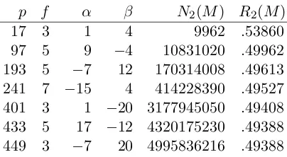
Table 2: Examples from Cyclotomy
p f α β N2(M) R2(M)
17 3 1 4 9962 .53860
97 5 9 −4 10831020 .49962
193 5 −7 12 170314008 .49613
241 7 −15 4 414228390 .49527
401 3 1 −20 3177945050 .49408
433 5 17 −12 4320175230 .49388
449 3 −7 20 4995836216 .49388
Example 5.5. Suppose p = 17 = 4×4 + 1. Then ν = 3 is a primitive element. Since
17 = 12 + 42, we have α = 1 and β ∈ {4,13}. We compute 34 ≡ 13 mod 17. Since
1/4≡13 mod 17, we have β = 4. The cyclotomic classes are
C0 = {1,13,16,4}
C1 = {3,5,14,12}
C2 = {9,15,8,2}
C3 = {10,11,7,6}.
The cyclotomic numbers can now be computed from Theorem 5.6; they are
(0,0) =A0=
17−11−6
16 = 0
(1,1) =A1=
17−3 + 2−4×4
16 = 0
(2,2) =A2=
17−3 + 2
16 = 1
(3,3) =A3=
17−3 + 2 + 4×4
16 = 2.
The total number of invertible2 by 2 submatrices in M is9962.
It remains to consider the invertibility of the matrices M constructed above. The ma-trices in question are cyclic. Suppose ap by p cyclic 0−1 matrixM has as its initial row the vector (m0, . . . , mp−1). We associate with this vector the polynomial
m(x) = p−1
X
i=0
mixi ∈Z2[x].
It is easy to see thatM is invertible if and only if gcd(m(x), xp−1) = 1. In this case, the inverse m−1(x) of m(x) is defined in the quotient ring Z2[x]/(xp−1). The cyclic matrix
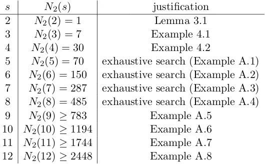
Table 3: Values and Bounds onN2(s) for small s
s N2(s) justification
2 N2(2) = 1 Lemma 3.1
3 N2(3) = 7 Example 4.1
4 N2(4) = 30 Example 4.2
5 N2(5) = 70 exhaustive search (Example A.1)
6 N2(6) = 150 exhaustive search (Example A.2)
7 N2(7) = 287 exhaustive search (Example A.3)
8 N2(8) = 485 exhaustive search (Example A.4)
9 N2(9)≥783 Example A.5
10 N2(10)≥1194 Example A.6
11 N2(11)≥1744 Example A.7
12 N2(12)≥2448 Example A.8
Example 5.6. Let p= 17. From Example 5.5, we have C0 ={1,13,16,4}. The first row
of M is
1 0 1 1 0 1 1 1 1 1 1 1 1 0 1 1 0,
which corresponds to the polynomial
m(x) = 1 +x2+x3+x5+x6+x7+x8+x9+x10+x11+x12+x14+x15.
The inverse of m(x) is
m−1(x) = 1 +x+x3+x4+x5+x6+x7+x10+x11+x12+x13+x14+x16.
By Dirichlet’s Theorem, there are an infinite number of primes p≡1 mod 8. However, we do not have a theoretical criterion to determine if a given matrix M in this class of examples is invertible. Therefore, we cannot prove that there are an infinite number of examples of this type. However, by computing gcds, as described above, we determined all the invertible matrices M of order less than 500 that can be constructed by this method. Some data about these matrices is presented in Table 2. Another observation is that, if this is in fact an infinite class, then it can be shown that the density of these examples approaches 63/128≈.492 asf approaches infinity.
5.6 Values and Bounds on N2(s) for Small s
We summarize our upper and lower bounds onN2(s) for s≤12 in Table 3. For the cases
s = 5,6,7,8, we have exact values of N2(s) that are obtained from exhaustive computer
6
General Transforms
In this section, we examine general (i.e., linear or nonlinear) AONT over an arbitrary alphabet, extending some results from [12] in a straightforward manner.
Let A be an N by k array whose entries are elements chosen from an alphabet X of orderv. We will refer toA as an (N, k, v)-array. Suppose the columns of Aare labelled by the elements in the setC={1, . . . , k}. Let D⊆C, and defineAD to be the array obtained from A by deleting all the columnsc /∈D. We say that A isunbiased with respect toD if the rows ofAD contain every|D|-tuple of elements ofX exactly N/v|D| times.
The following result characterizes (t, s, v)-AONT in terms of arrays that are unbiased with respect to certain subsets of columns.
Theorem 6.1. A (t, s, v)-AONT is equivalent to a (vs,2s, v)-array that is unbiased with respect to the following subsets of columns:
1. {1, . . . , s},
2. {s+ 1, . . . ,2s}, and
3. I∪ {s+ 1, . . . ,2s} \J, for all I ⊆ {1, . . . , s} with |I|=t and all J ⊆ {s+ 1, . . . ,2s}
with|J|=t.
Proof. Let A be the hypothesized (vs,2s, v)-array on alphabet X,|X|=v. We construct
φ:Xs→Xs as follows: for each row (x1, . . . , x2s) ofA, define
φ(x1, . . . , xs) = (xs+1, . . . , x2s).
The functionφ is easily seen to be a (t, s, v)-AONT.
Conversely, suppose φis a (t, s, v)-AONT. Define an array A whose rows consist of all
vs 2s-tuples (x1, . . . , x2s), where φ(x1, . . . , xs) = (xs+1, . . . , x2s). Then A is the desired
(vs,2s, v)-array.
An OA(s, k, v) (an orthogonal array) is a (vs, k, v)-array that is unbiased with respect to any subset ofs columns. The following corollary of Theorem 6.1 is immediate.
Corollary 6.2. If there exists an OA(s,2s, v), then there exists a (t, s, v)-AONT for all t
such that1≤t≤s.
7
Summary
We have initiated a study of all-or-nothing transforms where we consider the security of
t inputs when s− t outputs are fixed or known. We focussed on the case t = 2, for linear transformations defined overF2. Here one fundamental problem is to determine the
maximum 2-density, which we denoted byR2(s). We ask if lims→∞R2(s) exists, and if so,
what its value is. Our results establish that, if this limitLexists, then.494≤L≤.625. It should be possible to adapt the techniques used in this paper to deal with cases where
Acknowledgements
D. R. Stinson would like to thank Jeroen van de Graaf for rekindling his interest in AONT. Thanks also to Hugh Williams for providing some relevant number-theoretic information, and to Yuying Li and Henry Wolkowicz for useful discussions about quadratic programming.
References
[1] V. Canda and Tran van Trung. A new mode of using all-or-nothing transforms.ISIT 2002, p. 296
[2] R. Canetti, Y. Dodis, S. Halevi, E. Kushilevitz and A. Sahai. Exposure-resilient func-tions and all-or-nothing transforms.Lecture Notes in Computer Science1807(2000), 453–469 (EUROCRYPT 2000).
[3] R. G. Cascella, Z. Cao, M. Gerla, B. Crispo and R. Battiti. Weak data secrecy via obfuscation in network coding based content distribution. Wireless Days, 2008, pp. 1–5.
[4] C. J. Colbourn and J. H. Dinitz, eds.The CRC Handbook of Combinatorial Designs, Second Edition, CRC Press, 2006.
[5] A. Desai. The security of all-or-nothing encryption: protecting against exhaustive key search.Lecture Notes in Computer Science 1880(2000), 359–375 (CRYPTO 2000).
[6] Q. Guo, M. Luo, L. Li and Y. Yang. Secure network coding against wiretapping and Byzantine attacks.EURASIP Journal on Wireless Communications and Networking
2010(2010), article No. 17.
[7] S. A. Katre and A. R. Rajwade. Resolution of the sign ambiguity in the determination of the cyclotomic numbers of order 4 and the corresponding Jacobsthal sum. Math. Scand.60(1987), 52–62.
[8] J. Liu, H. Wang, M. Xian and K. Huang. A secure and efficient scheme for cloud storage against eavesdropper.Lecture Notes in Computer Science8233(2013), 75–89 (ICICS 2013).
[9] A. Proano and L. Lazos. Packet-hiding methods for preventing selective jamming attacks.IEEE Transactions on Dependable and Secure Computing9(2012), 101–114.
[10] R. L. Rivest. All-or-nothing encryption and the package transform. Lecture Notes in Computer Science1267(1997), 210–218 (Fast Software Encryption 1997).
[11] Y.-J. Song, K.-Y. Park and J.-M. Kang. The method of protecting privacy capa-ble of distributing and storing of data efficiently for cloud computing environment.
Computers, Networks, Systems and Industrial Engineering 2011, pp. 258–262.
[13] M. Tawarmalani and N. V. Sahinidis. A polyhedral branch-and-cut approach to global optimization.Mathematical Programming 103 (2005), 225–249.
[14] R. A. Vasudevan , A. Abraham and S. Sanyal. A novel scheme for secured data transfer over computer networksJournal of Universal Computer Science11 (2005), 104–121.
[15] Q. Zhang and L. Lazos. Collusion-resistant query anonymization for location-based services.2014 IEEE International Conference on Communications, pp. 768–774.
A
Matrices Yielding Good or Exact Lower Bounds for
N
2(
M
)
Example A.1. An invertible5 by 5 matrix having70 invertible 2×2 submatrices:
M5×5=
0 0 1 1 1
0 1 0 1 1
1 0 0 1 1
1 1 1 0 1
1 1 1 1 0
.
Example A.2. An invertible6 by 6 matrix having150 invertible2×2 submatrices:
M6×6 =
0 0 1 1 1 1
0 1 0 1 1 1
1 0 1 0 1 1
1 1 0 1 0 1
1 1 1 0 0 1
1 1 1 1 1 0
.
Example A.3. An invertible7 by 7 matrix having287 invertible2×2 submatrices:
M7×7 =
0 0 1 1 1 1 1
0 1 0 1 1 1 1
1 0 1 0 1 1 1
1 1 0 1 0 1 1
1 1 1 0 1 0 1
1 1 1 1 0 1 0
1 1 1 1 1 0 0
Example A.4. An invertible8 by 8 matrix having485 invertible2×2 submatrices:
M8×8 =
0 0 0 1 1 1 1 1
0 1 1 0 1 1 1 1
0 1 1 1 0 1 1 1
1 0 1 0 1 1 1 1
1 1 0 1 0 1 1 1
1 1 1 1 1 0 0 1
1 1 1 1 1 0 1 0
Example A.5. An invertible9 by 9 matrix having783 invertible2×2 submatrices:
M9×9 =
0 0 0 1 1 1 1 1 1
0 1 1 0 0 1 1 1 1
0 1 1 1 1 0 0 1 1
1 0 1 0 1 0 1 1 1
1 0 1 1 0 1 1 0 1
1 1 0 1 0 1 0 1 1
1 1 0 1 1 1 1 0 0
1 1 1 0 1 1 0 0 1
1 1 1 1 1 0 1 1 0
Example A.6. An invertible10 by 10 matrix having 1194invertible 2×2 submatrices:
M10×10=
0 0 0 1 1 1 1 1 1 1
0 1 1 0 1 1 0 1 1 1
0 1 1 1 0 1 1 0 1 1
1 0 1 1 1 0 1 1 0 1
1 1 0 1 1 1 0 1 1 1
1 1 1 0 1 1 1 0 1 1
1 0 1 1 0 1 1 1 0 1
1 1 0 1 1 0 1 1 1 0
1 1 1 0 1 1 0 1 1 0
1 1 1 1 1 1 1 0 0 0
Example A.7. An invertible11 by 11 matrix having 1744invertible 2×2 submatrices:
M11×11=
0 0 0 1 1 1 1 1 1 1 0
0 1 1 0 1 0 1 1 1 0 1
0 1 1 1 0 1 1 0 1 1 1
1 0 1 1 1 0 1 1 0 1 1
1 1 0 1 1 1 0 1 1 1 1
1 1 1 0 1 1 1 0 1 0 1
1 1 0 1 0 1 1 1 0 1 1
1 0 1 1 1 0 1 1 1 0 1
1 1 1 1 0 1 0 1 1 1 0
1 0 1 0 1 1 1 0 1 1 0
0 1 1 1 1 1 1 1 0 0 0
Example A.8. An invertible12 by 12 matrix having 2448invertible 2×2 submatrices:
M12×12=
1 0 1 1 1 1 1 1 1 0 1 0
1 1 1 1 1 0 1 1 1 1 1 0
1 1 1 0 1 0 1 1 0 1 1 1
0 0 1 0 1 1 1 0 1 1 1 1
0 0 1 1 1 1 1 1 0 1 0 1
1 1 0 1 1 0 0 1 1 1 1 1
0 1 1 0 0 1 1 0 1 1 1 1
0 1 0 1 1 1 0 1 1 1 0 1
0 1 1 1 0 1 1 1 1 1 1 0
1 1 1 1 1 1 0 1 0 0 1 1
1 1 1 0 1 1 1 1 1 1 0 1
1 1 0 1 1 1 1 0 1 0 0 1