Practical, Predictable Lattice Basis Reduction
∗Daniele Micciancio UCSD
Michael Walter UCSD
Abstract
Lattice reduction algorithms are notoriously hard to predict, both in terms of running time and output quality, which poses a major problem for cryptanalysis. While easy to analyze algorithms with good worst-case behavior exist, previous experimental evidence suggests that they are outperformed in practice by algorithms whose behavior is still not well understood, despite more than 30 years of intensive research. This has lead to a situation where a rather complex simulation procedure seems to be the most common way to predict the result of their application to an instance. In this work we present new algorithmic ideas towards bridging this gap between theory and practice. We report on an extensive experimental study of several lattice reduction algorithms, both novel and from the literature, that shows that theoretical algorithms are in fact surprisingly practical and competitive. In light of our results we come to the conclusion that in order to predict lattice reduction, simulation is superfluous and can be replaced by a closed formula using weaker assumptions.
One key technique to achieving this goal is a novel algorithm to solve the Shortest Vector Problem (SVP) in the dual without computing the dual basis. Our algorithm enjoys the same practical efficiency as the corresponding primal algorithm and can be easily added to an existing implementation of it.
1
Introduction
Lattice basis reduction is a fundamental tool in cryptanalysis and it has been used to successfully attack many cryptosystems, based on both lattices, and other mathematical problems. (See for example [9, 23, 39, 44–47, 61, 62, 66].) The success of lattice techniques in cryptanalysis is due to a large extent to the fact that reduction algorithms perform much better in practice than predicted by their theoretical worst-case analysis. Basis reduction algorithms have been investigated in many papers over the past 30 years [3, 6, 8, 10, 12–16, 18, 20, 21, 26, 28, 32, 36, 40–42, 45, 48, 50, 51, 54–56, 58– 60, 63, 65, 67–69], but the gap between theoretical analysis and practical performance is still largely unexplained. This gap hinders our ability to estimate the security of lattice based cryptographic functions, and it has been widely recognized as one of the main obstacles to the use of lattice cryptography in practice. In this work, we make some modest progress towards this challenging goal.
By and large, the current state of the art in lattice basis reduction (in theory and in practice) is represented by two algorithms:
∗
• the eminently practical Block-Korkine-Zolotarev (BKZ) algorithm of Schnorr and Euchner [54, 60], in its modern BKZ 2.0 incarnation [8] incorporating pruning, recursive preprocessing and early termination strategies [14, 18],
• the Slide reduction algorithm of Gama and Nguyen [15], an elegant generalization of LLL [27, 40] which provably approximates short lattice vectors within factors related to Mordell’s inequality.
Both algorithms make use of a Shortest Vector Problem (SVP) oracle for lower dimensional lattices, and are parameterized by a bound k (called the “block size”) on the dimension of these lattices. The Slide reduction algorithm has many attractive features: it makes only a polynomial number of calls to the SVP oracle, all SVP calls are to projected sub-lattices in exactly the same dimension k, and it achieves the best known worst-case upper bound on the length of its shortest output vector: γk(n−1)/(2(k−1))det(L)1/n, where γ
k = Θ(k) is the Hermite constant, and det(L) is the determinant of the lattice. Unfortunately, it has been reported [15, 16] that in experiments the Slide reduction algorithm is outperformed by BKZ, which produces much shorter vectors for comparable block size. In fact, [15] remarks that even BKZ with block sizek= 20 produces better reduced bases than Slide reduction with block size k= 50. As a consequence, the Slide reduction algorithm is never used in practice, and it has not been implemented and experimentally tested beyond the brief claims made in the initial work [15, 16].1
On the other hand, while surprisingly practical in experimental evaluations, the BKZ algorithm has its own shortcomings too. In its original form, BKZ is not even known to terminate after a polynomial number of calls to the SVP oracle, and its observed running time has been reported [16] to grow superpolynomially in the lattice dimension, even when the block size is fixed to some relatively small value k ≈ 30. Even upon termination, the best provable bounds on the output quality of BKZ are worse than Slide reduction by at least a polynomial factor [15].2 In practice, in order to address running time issues, BKZ is often employed with an “early termination” strategy [8] that tries to determine heuristically when no more progress is expected from running the algorithm. Theoretical bounds on the quality of the output after a polynomial number of iterations have been proved [18], but they are worse than Slide reduction by even larger polynomial factors. Another fact that complicates the analysis (both in theory and in practice) of the output quality of BKZ is the fact that the algorithm makes SVP calls in all dimensions up to the block size. In theory, this results in a formula that depends on all worst-case (Hermite) constantsγifori≤k. In practice, the output quality and running time is evaluated by a simulator [8] that initially attempts to numerically estimate the performance of the SVP oracle on random lattices in all possible dimensions up tok.
Our Contribution We introduce new algorithmic techniques that can be used to design improved lattice basis reduction algorithms, analyze their theoretical performance, implement them, and report on their practical behavior through a detailed set of experiments with block size as high as 75, and several data points per dimension for (still preliminary, but already meaningful) statistical estimation.
1While we are referencing two separate works, both refer to the same experimental study. 2
One of our main findings is that the Slide reduction algorithm is much more practical than originally thought, and as the dimension increases, it performs almost as well as BKZ, while at the same time, offering a simple closed-formula to evaluate its output quality. This provides a simple and effective method to evaluate the impact of lattice basis reduction attacks on lattice cryptography, without the need to run simulators or other computer programs [8, 68]. Key to our findings, is a new procedure to enumerate shortest lattice vectors indual lattices, without the need to explicitly compute a dual basis. Interestingly, our dual enumeration procedure is almost identical (syntactically) to the standard enumeration procedure to find short vectors in a (primal) lattice, and, as expected, it is just as efficient in practice. Using our new procedure, we are able to conduct experiments using Slide reduction with significantly larger block size than previously reported, and observe that the gap between theoretical (more predicable) algorithms and practical heuristics gets pretty narrow already for moderate block size and dimension.
For small block sizes (say, up to 40), there is still a substantial gap between the output quality of Slide reduction and BKZ in practice. For this setting, we design a new variant of BKZ, based on lattice duality and a new notion of block reduced basis. Our new DBKZ algorithm can be efficiently implemented using our dual enumeration procedure, achieving running times comparable to BKZ, and matching its experimental output quality for small block size almost exactly. (See Figure 5.) At the same time, our algorithm has various advantages over BKZ, that make it a better target for theoretical analysis: it only makes calls to an SVP oracle in fixed dimensionk, and it is self dual, in the sense that it performs essentially the same operations when run on a basis or its dual. The fact that all SVP calls on projected sublattices are in the same fixed dimensionkhas several important implications. First, it results in a simpler bound on the length of the shortest output vector, which can be expressed as a function of justγk. More importantly, this allows to get a practical estimate on the output quality simply by replacing γk with the value predicted by the Gaussian Heuristic
GH(k), commonly used in lattice cryptanalysis. We remark that the GH(k) formula has been validated for moderately large values of k, where it gives fairly accurate estimates on the shortest vector length ink-dimensional sublattices. However, early work on predicting lattice reduction [16] has also shown that for small k (say, up to k ≤25), BKZ sublattices do not follow the Gaussian Heuristic. As a result, while the BKZ 2.0 simulator of [8] makes extensive use of GH(k) for large values ofk, it also needs to resort to cumbersome experimental estimations for predicting the result of SVP calls in dimension lower than k. By making only SVP calls on k-dimensional sublattices, our algorithm obviates the need for any such experimental estimates, and allows to predict the output quality (under the same, or weaker heuristic assumptions than the BKZ 2.0 simulator) just using the GH(k) formula. We stress that this is not only true for the length of the shortest vector found by our algorithm, but one can estimate many more properties of the resulting basis. This is important in many cryptanalytic settings, where lattice reduction is used as a preprocessing for other attacks. In particular, using the Gaussian Heuristic we are able to show that a large part of the basis output by our algorithm can be expected to follow the Geometric Series Assumption [57], an assumption often made about the output of lattice reduction, but so far never proven. (See Section 5 for details.) One last potential advantage of only making SVP calls in fixed dimensionk
Technical ideas Enumeration algorithms (as typically used within block basis reduction) find short vectors in a lattice by examining all possible coordinatesx1, . . . , xn of candidate short lattice vectors P
ibi ·xi with respect to the given lattice basis, and using the length of the projected lattice vector to prune the search. Our dual lattice enumeration algorithm works similarly, but without explicitly computing a basis for the dual lattice. The key technical idea is that one can enumerate over the scalar products yi = hbi,vi of the candidate short dual vectors v and the primal basis vectors bi.3 Perhaps surprisingly, one can also compute the length of the projections of the dual lattice vectorv(required to prune the enumeration tree), without explicitly computing
v or a dual basis. The simplicity of the algorithm is best illustrated just by looking at the pseudo code, and comparing it side-to-side to the pseudo code of standard (primal) lattice enumeration. (See Algorithms 2 and 3 in Section 7.) The two programs are almost identical, leading to a dual enumeration procedure that is just as efficient as primal enumeration, and allowing the application of all standard optimizations (e.g., all various forms of pruning) that have been developed for enumerating in primal lattices.
On the basis reduction front, our DBKZ algorithm is based on a new notion of block-reduced basis. Just as for BKZ, DBKZ-reduction is best described as a recursive definition. In fact, the recursive condition is essentially the same for both algorithms: given a basis B, if b is a shortest vector in the sublattice generated by the first k basis vectors B[1,k], we require the projection of B orthogonal to b to satisfy the recursive reduction property. The difference between BKZ and DBKZ is that, while BKZ requires B[1,k] to start with a shortest lattice vector b =b1, in DBKZ
we require it to end with a shortest dual vector.4 This simple twist in the definition of reduced basis leads to a much simpler bound on the length ofb, improving the best known bound for BKZ reduction, and matching the theoretical quality of Slide reduction.
Experiments To the best of our knowledge, we provide the first experimental study of lattice reduction with large block size parameter beyond BKZ. Even for BKZ we improve on the currently only study involving large block sizes [8] by collecting multiple data points per block size parameter. This allows us to apply standard statistical methods to try to get a sense of the main statistical parameters of the output distribution. Clearly, learning more about the output distribution of these algorithms is highly desirable for cryptanalysis, as an adversary is drawing samples from that distribution and will utilize the most convenient sample, rather than a sample close to the average. Finally, in contrast to previous experimental work [8, 16], we contribute to the community by making our code5 and data6 publicly available. To the best of our knowledge, this includes the first publicly available implementation of dual SVP reduction and Slide reduction. At the time of publication of this work, a modified version of our implementation of dual SVP reduction has been integrated into the main branch of fpLLL[4]. We hope that this will spur more research into the predictability of lattice reduction algorithms.
3
By definition of dual lattice, all these productsyi are integers, and, in fact, they are the coordinates ofv with respect to the standarddual basis ofb1, . . . ,bn.
4
To be precise, we requireb∗k/kb ∗ kk
2
to be a shortest vector in the dual lattice ofB[1,k]. See Section 3 for details. 5
http://cseweb.ucsd.edu/~miwalter/src/fplll-dual_enum/fplll-dual_enum.zip
6
2
Preliminaries
Notation Numbers and reals are denoted by lower case letters. For n ∈ Z+ we denote the set
{0, . . . , n} by [n]. For vectors we use bold lower case letters and the i-th entry of a vector v is denoted by vi. Lethv,wi=Pivi·wi be the scalar product of two vectors. If p≥1 we define the
p norm of a vector v to be kvkp = (P|
vi|p)1/p. We will only be concerned with the norms given by p = 1, 2, and ∞. Whenever we omit the subscript p, we mean the standard Euclidean norm, i.e. p= 2. We define the projection of a vectorb orthogonal to a vector v asπv(b) =b−hkbv,kv2iv.
Matrices are denoted by bold upper case letters. Thei-th column of a matrixB is denoted bybi. Furthermore, we denote the submatrix comprising the columns from the i-th to the j-th column (inclusive) as B[i,j] and the horizontal concatenation of two matrices B1 and B2 by [B1|B2]. For
any matrix B and p≥1 we define the induced norm to be kBkp = maxkxkp=1(kBxkp). Forp= 1 (resp. ∞) this is often denoted by the column (row) sum norm; forp= 2 this is also known as the spectral norm. It is a classical fact that kBk2 ≤p
kBk1kBk∞. Finally, we extend the projection operator to matrices, where πV(B) is the matrix obtained by applying πV to every column bi of
B and πV(bi) =πvk(· · ·(πv1(bi))· · ·).
2.1 Lattices
A lattice Λ is a discrete subgroup of Rm and is generated by a matrix B ∈ Rm×n, i.e. Λ = L(B) ={Bx: x∈Zn}. If B has full column rank, it is called abasis of Λ and dim(Λ) =n is the dimension (or rank) of Λ. A lattice has infinitely many bases, which are related to each other by right-multiplication with unimodular matrices. With each matrixBwe associate its Gram-Schmidt-Orthogonalization (GSO) B∗, where the i-th column b∗i of B∗ is defined as b∗i = πB∗[1,i−1](bi) =
bi−Pj<iµi,jbj∗andµi,j =hbi,b∗ji/kb∗jk2 (andb∗1 =b1). For every lattice basis there are infinitely
many bases that have the same GSO vectors b∗i, among which there is a (not necessarily unique) basis that minimizeskbikfor all i. Transforming a basis into this form is commonly known assize
reduction and is easily and efficiently done using a slight modification of the Gram-Schmidt process. In this work we will implicitly assume all bases to be size reduced. The reader can simply assume that any basis operation described in this work is followed by a size reduction. For a fixed matrix
B we extend the projection operation to indices: πi(·) =πB∗
[1,i−1](·), so π1(B) =B. Whenever we
refer to the shape of a basisB, we mean the vector (kb∗ik)i∈[n]. We defineD† to be the GSO of D
in reverse order.
For every lattice Λ there are a few invariants associated to it. One of them is its determinant det(L(B)) =Q
ikb
∗
ik for any basis B. Even though the basis of a lattice is not uniquely defined, the determinant is and it is efficiently computable given a basis. Furthermore, for every lattice Λ we denote the length of its shortest non-zero vector (also known as the first minimum) by
λ1(Λ), which is always well defined. We use the short-hand notations det(B) = det(L(B)) and
λ1(B) = λ1(L(B)). Minkowski’s theorem is a classic result that relates the first minimum to the
determinant of a lattice. It states that λ1(Λ)≤
√
γndet(Λ)1/n, for any Λ with dim(Λ) =n, where Ω(n) ≤ γn ≤ n is Hermite’s constant. Finding a (even approximate) shortest nonzero vector in a lattice, commonly known as the Shortest Vector Problem (SVP), is NP-hard under randomized reductions [25, 34].
satisfies span(B) = span(D) andBTD=DTB =I. Then L([B) =L(D) and we denote D as the
dual basis ofB. It follows that for any vectorw=Dx we have thatBTw=x, i.e. we can recover the coefficients x of w with respect to the dual basis D by multiplication with the transpose of the primal basis BT. Given a lattice basis, its dual basis is computable in polynomial time, but requires at least Ω(n3) bit operations using matrix inversion. Finally, if D is the dual basis of B, their GSOs are related bykb∗ik= 1/kd†ik.
In this work we will often modify a lattice basis B such that its first vector satisfiesαkb1k ≤
λ1(B) for some α ≤ 1. We will call this process SVP reduction of B. Given an SVP oracle, it
can be accomplished by using the oracle to find the shortest vector in L(B), prepending it to the basis, and running LLL (cf. Section 2.3) on the resulting generating system. Furthermore, we will modify a basis B such that its dual D satisfies αkdnk ≤ λ1(L([B)), i.e. its reversed dual basis is
SVP reduced. This process is called dual SVP reduction. Note that if B is dual SVP reduced, then kb∗nk is maximal among all bases of L(B). The obvious way to achieve dual SVP reduction is to compute the dual of the basis, SVP reduce it as described above, and compute the primal basis. We present an alternative way to achieve this in Section 7. In the context of reduction algorithms, the relaxation factorα is usually needed for proofs of termination or running time and only impacts the analysis of the output quality in lower order terms. In this work, we will sweep it under the rug and take it implicitly to be a constant close to 1. Finally, we will apply SVP and dual SVP reduction to projected blocks of a basis B, for example we will (dual) SVP reduce the blockπi(B[i,i+k]). By that we mean that we will modifyB in such a way thatπi(B[i,i+k]) is (dual)
SVP reduced. This can easily be achieved by applying the transformations to the original basis vectors instead of their projections.
2.2 Enumeration Algorithms
In order to solve SVP in practice, enumeration algorithms are usually employed, since these are the most efficient algorithms for currently realistic dimensions. The standard enumeration procedure, usually attributed to Fincke, Pohst [11], and Kannan [24] can be described as a recursive algorithm: given as input a basis B∈Zm×nand a radius r, it first recursively finds all vectorsv0 ∈ L(π
2(B))
withkv0k ≤r, and then for each of them finds allv∈ L(B), s.t. π2(v) =v0 andkvk ≤r, usingb1.
This essentially corresponds to a breadth first search on a large tree, where layers correspond to basis vectors and the nodes to the respective coefficients. While it is conceptually simpler to think of enumeration as a BFS, implementations usually employ a depth first search for performance reasons. Pseudo code can be found in Algorithm 3 in Section 7.
There are several practical improvements of this algorithm collectively known as SchnorrEuch-ner enumeration [60]: First, due to the symmetry of lattices, we can reduce the search space by ensuring that the last non zero coefficient is always positive. Furthermore, if we find a vector shorter than the boundr, we can update the latter. And finally, we can enumerate the coefficients of a basis vector in order of the length of the resulting (projected) vector and thus increase the chance of finding some short vector early, which will update the boundr and keep the search space smaller.
2.3 Lattice Reduction
As opposed to exact SVP algorithms, lattice reductions approximate the shortest vector. The quality of their output is usually measured in the length of the shortest vector they are able to find with respect to the root determinant of the lattice. This quantity is denoted by theHermite factor
¯
δ=kb1k/det(B)1/n. The Hermite factor depends on the lattice dimensionn, but the experiments
of [16] suggest that the root Hermite factor δ = ¯δ1/n converges to a constant as n increases for popular reduction algorithms. During our experiments we found that to be true at least for large enough dimensions (n≥140).
The LLL algorithm [27] is a polynomial time basis reduction algorithm. A basis B ∈ Zm×n can be defined to be LLL reduced if B[1,2] is SVP reduced and π2(B) is LLL reduced. From
this it is straight forward to prove that LLL reduction achieves a root Hermite factor of at most
δ≤γ21/4≈1.0746. However, LLL has been reported to behave much better in practice [16, 43].
BKZ [54] is a generalization of LLL to larger block size. A basisB is BKZ reduced with block size k (denoted by BKZ-k) if B[1,min(k,n)] is SVP reduced and π2(B) is BKZ-k reduced. BKZ
achieves this by simply scanning the basis from left to right and SVP reducing each projected block of size k (or smaller once it reaches the end) by utilizing a SVP oracle for all dimensions≤k. It iterates this process (which is usually called atour) until no more change occurs. Whenk=n, this is usually referred to asHKZ reduction and is essentially equivalent to solving SVP. The following bound for the Hermite factor holds for b1 of a BKZ-kreduced basis [18]:
kb1k ≤2γ n−1 2(k−1)+
3 2
k det(B)
1/n (1)
Equation (1) shows that the root Hermite factor achieved by BKZ-kis at most .γ
1 2(k−1)
k .
Further-more, while there is no polynomial bound on the number of calls BKZ makes to the SVP oracle, Hanrot, Pujol, and Stehl´e showed in [18] that one can terminate BKZ after a polynomial number of calls to the SVP oracle and still provably achieve the bound (1). Finally, BKZ has been repeatedly reported to behave very well in practice [8, 16]. For these reasons, BKZ is very popular in practice and implementations are readily available in different libraries, e.g. inNTL[64] or fpLLL [4].
In [15], Gama and Nguyen introduced a different block reduction algorithm, namely Slide re-duction. It is also parameterized by a block sizek, which is required to divide the lattice dimension
n, but uses a SVP oracle only in dimension k. 7 A basis B is defined to be slide reduced, if
B[1,k] is SVP reduced, π2(B[2,k+1]) is dual SVP reduced (if k > n), and πk+1(B[k+1,n]) is slide
reduced. Slide reduction, as described in [15], reduces a basis by first alternately SVP reducing all blocks πik+1(B[ik+1,(i+1)k]) and running LLL on B. Once no more changes occur, the blocks
πik+2(B[ik+2,(i+1)k+1]) are dual SVP reduced. This entire process is iterated until no more changes
occur. Upon termination, the basis is guaranteed to satisfy
kb1k ≤γ n−1 2(k−1)
k det(B)
1/n (2)
This is slightly better than Equation (1), but the achieved root Hermite factor is also only
guar-anteed to be less than γ
1 2(k−1)
k . Slide reduction has the desirable properties of only making a
7Strictly speaking, the algorithm as described in [15] uses HKZ reduction and thus requires an SVP oracle in lower
polynomial number of calls to the SVP oracle and that all calls are in dimension k (and not in lower dimensions). The latter allows for a cleaner analysis, for example when combined with the Gaussian Heuristic (cf. Section 2.4). Unfortunately, Slide reduction has been reported to be greatly inferior to BKZ in experiments [16], so it is rarely used in practice and we are not aware of any publicly available implementation.
2.4 The Gaussian Heuristic
The Gaussian Heuristic gives an approximation of the number of lattice points in a “nice” subset of
Rn. More specifically, it says that for a given setSand a lattice Λ, we have|S∩Λ| ≈vol(S)/det(Λ). The heuristic has been proved to be very useful in the average case analysis of lattice algorithms. For example, it can be used to estimate the complexity of enumeration algorithms [14, 19] or the output quality of lattice reduction algorithms [8]. For the latter, note that reduction algorithms work by repeatedly computing the shortest vector in some lattice and inserting this vector in a certain position of the basis. To estimate the effect such a step has on the basis, it is useful to be able to predict how long such a vector might be. This is where the Gaussian Heuristic comes in: using the above formula, one can estimate how large the radius of an n-dimensional ball (this is the “nice” set) needs to be such that we can expect it to contain a non-zero lattice point (where
n = dim(Λ)). Using the volume formula for the n-dimensional ball, we get an estimate for the shortest non-zero vector in a lattice Λ:
GH(Λ) = (Γ(n/2 + 1)·det(Λ))
1/n √
π (3)
If k is an integer, we define GH(k) to be the Gaussian Heuristic (i.e. Equation (3)) for k -dimensional lattices with unit determinant. The heuristic has been tested experimentally [14], also in the context of lattice reduction [8, 16], and been found to be too rough in small dimensions, but to be quite accurate starting in dimension >45. In fact, for a precise definition of random lattices (which we are not concerned with in this work) it can be shown that the expected value of the first minimum of the lattice (over the choice of the lattice) converges to Equation (3) as the lattice dimension tends to infinity.8
Heuristic 1 [Gaussian Heuristic]For a given lattice Λ, λ1(Λ) =GH(Λ).
Invoking Heuristic 1 for all projected sublattices that the SVP oracle is called on during the process, the root Hermite factor achieved by lattice reduction (usually with regards to BKZ) is commonly estimated to be [5]
δ≈GH(k)k−11. (4)
However, since the Gaussian Heuristic only seems to hold in large enough dimensions and BKZ makes calls to SVP oracles in all dimensions up to the block sizek, it is not immediately clear how justified this estimation is. While there is a proof by Chen [7] that under the Gaussian Heuristic, Equation (4) is accurate for BKZ, this is only true as the lattice dimension tends to infinity. It might be reasonable to assume that this also holds in practice as long as the lattice dimension is
8One can also formulate Heuristic 1 for a given lattice by assuming it “behaves like a random lattice”. Depending
large enough compared to the block size, but in practice and cryptanalytic settings this is often not the case. In fact, in order to achieve an approximation good enough to break a cryptosystem, a block size at least linear in the lattice dimension is often required. As another approach to predicting the output of BKZ, Chen and Nguyen proposed a simulation routine [8]. Unfortunately, the simulator approach has several drawbacks. Obviously, it requires more effort to apply than a closed formula like (4), since it needs to be implemented and “typical” inputs need to be generated or synthesized (among others, the shape of a “typical” HKZ reduced basis in dimension 45). On top of that, the accuracy of the simulator is based on several additional heuristic assumptions, the validity of which has not been independently verified.
To the best of our knowledge there have been no attempts to make similar predictions for Slide reduction, as it is believed to be inferior to BKZ and thus usually not considered for cryptanalysis.
3
Self-Dual BKZ
In this section we describe our new reduction algorithm. Like BKZ it is parameterized by a block sizekand a SVP oracle in dimension k, and acts on the input basisB∈Zm×n by iterating tours. The beginning of every tour is exactly like a BKZ tour, i.e. SVP reducing every blockπi(B[i,i+k−1])
from i = 1 to n−k+ 1. We will call this part a forward tour. For the last block, which BKZ simply HKZ reduces and where most of the problems for meaningful predictions stem from, we do something different. Instead, we dual SVP the last block and proceed by dual SVP reducing all blocks of sizekbackwards (which is abackward tour). After iterating this process (which we call a
tour of Self-Dual BKZ) the algorithm terminates when no more progress is made. The algorithm is formally described in Algorithm 1.
Algorithm 1 Self-Dual BKZ
procedure DBKZ (B,k,SVPk)
Input: A lattice basis B∈Zm×n, a block size k, a SVP oracle in dimension k
Output: A k-reduced basisB0 (See Definition 1 for a formal definition.)
1 do
2 fori= 1. . . n−k
3 SVP reduce πi(B[i,i+k−1]) using SVPk
4 fori=n−k+ 1. . .1
5 dual SVP reduceπi(B[i,i+k−1]) usingSVPk
6 while progress is made
7 returnB
Note that, like BKZ, Self-Dual BKZ (DBKZ) is a proper block generalization of the LLL algo-rithm, which corresponds to the case k= 2.
The terminating condition in Line 6 is left ambiguous at this point on purpose as there are several sensible ways to approach this as we will see in the next section. One has to be careful to, on the one hand guarantee termination, while on the other hand achieving a meaningful reducedness definition.
3.1 Analysis
Definition 1 A basis B = [b1, . . . ,bn] is k-reduced if either n < k, or it satisfies the following
conditions:
• kb∗kk−1 =λ
1(L(\B[1,k])), and
• for some SVP reduced basis B˜ of L(B[1,k]), π2([ ˜B|B[k+1,n]]) is k-reduced.
We first prove that Algorithm 1 indeed achieves Definition 1 when used with a specific termi-nating condition:
Lemma 1 Let B be an n-dimensional basis. If πk+1(B) is the same before and after one loop of
Algorithm 1, thenB isk-reduced.
Proof The proof is inductive: for n = k the result is trivially true. So, assume n > k, and that the result already holds for n−1. At the end of each iteration, the first block B[1,k] is dual-SVP reduced by construction. So, we only need to verify that for some ˜B an SVP reduced basis for L(B[1,k), the projection π2([ ˜B|B[k+1,n]]) is also k-reduced. Let ˜B be the SVP reduced
basis produced in the first step. Note that the first and last operation in the loop do not change L(B[1,k]) and B[k+1,n]. It follows that πk+1(B) is the same before and after the partial tour (the
tour without the first and the last step) on the projected basis π2([ ˜B|B[k+1,n]]), and soπk+2(B) is
the same before and after the partial tour. By induction hypothesis,π2([ ˜B|B[k+1,n]]) isk-reduced.
2
Lemma 1 gives a terminating condition which ensures that the basis is reduced. We remark that it is even possible to adapt the proof such that it is sufficient to check that the shape of the projected basis πk+1(B) is the same before and after the tour, which is much closer to what one
would do in practice to check ifprogress was made (cf. Line 6). However, this requires to relax the definition of SVP-reduction slightly, such that the first vector is not necessarily a shortest vector, but merely a short vector achieving Minkowski’s bound. Since this is the only property of SVP reduced bases we need for the analysis below, this does not affect the worst case output quality. Finally, we are aware that it is not obvious that either of these conditions are ever met, e.g. (the shape of) πk+1(B) might loop indefinitely. However, in Section 4 we show that one can put a
polynomial upper bound on the number of loops without sacrificing worst case output quality. To show that the output quality of Self-Dual BKZ in the worst case is at least as good as BKZ’s worst case behavior, we analyze the Hermite factor it achieves:
Theorem 1 If B isk-reduced, thenλ1(B[1,k])≤
√
γk
n−1
k−1 ·det(B)1/n.
Proof Assume without loss of generality thatL(B) has determinant 1, and let ∆ be the determinant of L(B[1,k]). Let λ≤ √γk∆1/k and ˆλ≤
√
γk∆−1/k be the lengths of the shortest nonzero primal
and dual vectors ofL(B[1,k]). We need to prove thatλ≤
√
γk
n−1
k−1.
We first show, by induction onn, that the determinant ∆1 of the first k−1 vectors is at most
√
γkn−k+1det(B)(k−1)/n= √
γkn−k+1. SinceB is k-reduced, this determinant equals ∆1 = ˆλ·∆≤
√
γk∆1−1/k. (This alone already proves the base case of the induction forn=k.) Now, let ˜B be a SVP reduced basis of L(B[1,k]) satisfying thek-reduction definition, and consider the determinant
∆2= ∆/λofπ2( ˜B). Sinceπ2([ ˜B|B[k+1,n]]) has determinant 1/kb˜1k= 1/λ, by induction hypothesis
we have ∆2 ≤
√
∆ =λ∆2 ≤
√
γkn−kλ
n−k n−1 ≤√γ
kn−k( √
γk∆
1
k) n−k n−1 =√γ
k
(n−k)n n−1 ∆
n−k k(n−1).
Rising both sides to the power (n−1)/n we get ∆1−n1 ≤√γnn−k∆
1
k−
1
n, or, equivalently, ∆1−
1
k ≤
√
γkn−k. It follows that ∆1 = ˆλ∆≤
√
γk∆1−
1
k ≤√γkn−k+1, concluding the proof by induction.
We can now prove the main theorem statement. Recall from the inductive proof that ∆ ≤ √
γkn−kλ
n−k
n−1. Therefore,λ≤√γ
k∆1/k ≤ √
γk
n kλ
n−k
k(n−1). Solving forλ, proves the theorem. 2
4
Dynamical System
Proving a good running time on DBKZ directly seems just as hard as for BKZ, so in this section we analyze the DBKZ algorithm using the dynamical system technique from [18].
Let B = [b1, . . . ,bn] be an input basis to DBKZ, and assume without loss of generality that det(B) = 1. During a forward tour, our algorithm computes a sequence of lattice vectors
B0 = [b01, . . . ,b0n−k] where each b0i is set to a shortest vector in the projection of [bi, . . . ,bi+k−1]
orthogonal to [b01, . . . ,b0i−1]. This set of vectors can be extended to a basis B00 = [b001, . . . ,b00n] for the original lattice. Since [b01, . . . ,b0i−1] generates a primitive sublattice of [bi, . . . ,bi+k−1], the
projected sublattice has determinant det(L(b1, . . . ,bi+k−1))/det(L(b01, . . . ,b0i−1)), and the length
of its shortest vector is
k(b0i)∗k ≤√γk
det(L(b1, . . . ,bi+k−1))
det(L(b01, . . . ,b0i−1))
1/k
. (5)
At this point, simulations based on the Gaussian Heuristics typically assume that (5) holds with equality. In order to get a rigorous analysis without heuristic assumptions, we employ the amor-tization technique of [18, 19]. For every i = 1, . . . , n −k, let xi = log det(b1, . . . ,bk+i−1) and
x0i = log det(b01, . . . ,b0i). Using (5), we get for alli= 1, . . . , n−k,
x0i = x0i−1+ logk(b0i)∗k
≤ x0i−1+α+
xi−x0i−1
k
= ωx0i−1+α+ (1−ω)xi
whereω = (1−1/k),α= 21logγk and x00 = 0. By induction oni,
x0i≤α1−ω
i
1−ω + (1−ω)
i X
j=1
ωi−jxj,
or, in matrix notationx0 ≤b+Axwhere
b=αk
1−ω .. .
1−ωn−k
A=
1 k 1 ω 1 .. . . .. . .. ωn−k−1 · · · ω 1
Since all the entries ofA are positive, we also see that if Xi ≥xi are upper bounds on the initial valuesxi for alli, then the vectorX0=AX+b gives upper bounds on the output valuesx0i≤Xi0. The vector x0 describes the shape of the basis matrix before the execution of a backward tour. Using lattice duality, the backward tour can be equivalently formulated by the following steps:
1. Compute the reversed dual basisD of B0
2. Apply a forward tour toD to obtain a new dual basis D0
3. Compute the reversed dual basis ofD0
The reversed dual basis computation yields a basisD such that, for all i= 1, . . . , n−k,
yi = log det(d1, . . . ,dk+i−1)
= −log(det(B0)/det([b10, . . . ,b0n−k+1−i])) = log det([b01, . . . ,b0n−k+1−i]) =x0n−k+1−i.
So, the vector y describing the shape of the dual basis at the beginning of the backward tour is just the reverse ofx0. It follows that applying a full (forward and backward) DBKZ tour produces a basis such that if X are upper bounds on the log determinantsx of the input matrix, then the log determinants of the output matrix are bounded from above by
R(AR(AX+b) +b) = (RA)2X+ (RA+I)Rb
whereRis the coordinate reversal permutation matrix. This leads to the study of the discrete time affine dynamical system
X7→(RA)2X+ (RA+I)Rb. (6)
4.1 Output Quality
We first prove that this system has at most one fixed point.
Claim 1 The dynamical system (6) has at most one fixed point.
Proof Any fixed point is a solution to the linear system ((RA)2 −I)X+ (RA+I)Rb= 0. To prove uniqueness, we show that the matrix ((RA)2−I) is non-singular, i.e., if (RA)2x=x then x = 0. Notice that the matrix RA is symmetric, so we have (RA)2 = (RA)TRA = ATA. So proving ((RA)2−I) is non-singular is equivalent to showing that 1 is not an eigenvalue ofATA. We haveρ(ATA) =kAk2
2 ≤ kAk1kAk∞, whereρ(·) denotes the spectral radius of the given matrix (i.e. the largest eigenvalue in absolute value). But we also have
kAk∞=kAk1=
1
k
n−k−1
X
i=0
ωi = 1−ω n−k
k(1−ω) = 1−ω
n−k<1 (7)
which shows that the absolute value of any eigenvalue of ATA is strictly smaller than 1.2
Claim 2 The fixed point of the dynamical system x7→R(Ax+b) is given by
xi =
(n−k−i+ 1)(k+i−1)
k−1 α. (8)
Proof The unique fixed point of the system is given by the solution to the linear system (R−A)x=
b. We prove that (8) is a solution to the system by induction on the rows. For the first row, the system yields
xn−k−x1/k=α. (9)
From (8) we get that xn−k = nk−−11α and x1 =
k(n−k)
k−1 α. Substituting these into (9), the validity is
easily verified.
The r-th row of the system is given by
xn−k−r+1−
1 k r X j=1
ωr−jxj
=
1−ωr
1−ω α (10)
which is equivalent to
xn−k−r+1+ω
xn−k−r+2−
1
k
r−1
X
j=1
ωr−1−jxj
−
xr
k −ωxn−k−r+2 =
1−ωr
1−ω α. (11)
By induction hypothesis, this is equivalent to
ω
1−ωr−1
1−ω
α+xn−k−r+1−
xr
k −ωxn−k−r+2 =
1−ωr
1−ω α. (12)
Substituting (8) in fori=n−k−r+ 1, r, and n−k−r+ 2, we get
xn−k−r+1−
xr
k−ωxn−k−r+2=
kr(n−r)−(n−r−k+ 1)(r+k−1)−(k−1)(r−1)(n−r+ 1)
k(k−1) α
which, after some tedious, but straight forward, calculation can be shown to be equal toα (i.e. the fraction simplifies to 1). This in turn shows that the left hand side of (12) is equivalent to
ω
1−ωr−1
1−ω
α+α
which is equal to its right hand side. 2
Note that since x1 corresponds to the log determinant of the first block, applying Minkowski’s
theorem results in the same worst case Hermite factor as proved in Theorem 1.
4.2 Convergence
the difference is (RA)teand so its norm is bounded byk(RA)tekp≤ k(RA)tkpkekp≤ kRAkt pkekp. So if the induced norm of A is strictly smaller than 1, the corresponding norm of the error vector follows an exponential decay. While the spectral norm ofAseems hard to bound, the 1 and the in-finity norm are straight forward to analyze. In particular, we saw in (7) thatkAk∞= 1−ωn−k. This proves that the algorithm converges. Furthermore, let the input be a basis B (with det(B) = 1), the corresponding vector v = (log det(b1, . . . ,bk+i−1))1≤i≤n and write v =x+e. Then we have kek∞=kv−xk∞≤ kvk∞+kxk∞≤poly(n,size(B)). This implies that for
t= polylog(n,size(B))/ωn−k≈O(e(n−k)/k)polylog(n,size(B)) (13)
we have that k(RA)tek ≤ c for constant c. Equation (13) already shows that for k = Ω(n), the algorithm converges in a number of tours polylogarithmic in the lattice dimension n, i.e. makes at most ˜O(n) SVP calls. In the initial version of this work, proving polynomial convergence for arbitrary k was left as an open problem. Recently, Neumaier filled this gap [38]. In what follows we reformulate his proof using our notation for completeness, but we stress that this is originally Neumaier’s work.
Claim 3 Let x be the fixed point of the dynamical system as defined in Claim 2 and ri =ei/xi be
the relative error of the dynamical system. Then, ifr,r0 are the relative errors before and after the execution of one iteration of the system, thenkr0k∞≤(1−)krk∞ for= 1/(1 +n2/(4k(k−1)))≈ (2k/n)2. When k≥n/2, it is enough to take = (k−1)/(n−1).
Proof Assume without loss of generality that krk∞ = (k−1)/α, i.e., |ei| ≤ ((k−1)/α)xi = (n−k−i+ 1)(k+i−1) for all i = 1, . . . , n−k. We need to prove that |rj0| = |(RAe)j|/xj ≤ ((k−1)/α)(1−) for allj, or, equivalently,
|(Ae)j|=|(RAe)n−k−j+1| ≤
k−1
α (1−)xn−k−j+1 =j(n−j)(1−).
By the definition ofA, we have
|(Ae)j| ≤ 1
k
j X
i=1
ωj−i|ei| ≤ 1
k
j X
i=1
ωj−i(n−k−i+ 1)(k+i−1)≡f(j).
So, it is enough to prove that the functionf(j) on the right hand side satisfiesf(j)≤j(n−j)(1−). We prove this inequality by induction onj, under the assumption that
≤g(j)≡ k(k−1)
k(n−2j−1) +j(n−j).
• base case (j = 1): f(1) =n−k≤(n−1)(1−) if and only if ≤g(0) = (k−1)/(n−1).
• inductive step: assumef(j)≤j(n−j)(1−) by inductive hypothesis. We need to prove that
f(j+ 1) =ωf(j) +(n−k−j)(k+j)
k ≤
k−1
k j(n−j)(1−) +
(n−k−j)(k+j)
k
This concludes the inductive proof, as long as ≤g(j) forj = 0, . . . ,(n−k). Finally, we observe that the functiong(j) is minimized atj= n2−k, with minimumg(n2−k) = 1/(1 +n2/(4k(k−1))).
When k > n/2, the minimum is achieved at j <0 and g(j) is monotonically increasing for j≤0. So it is enough to take=g(0) = (k−1)/(n−1).2
By a similar argument as above, this shows that the error can be made arbitrarily close to 0 in
O((n/2k)2)polylog(n,size(B)) tours.
5
Heuristic Analysis
In the context of cryptanalysis, we are more interested in the average case behavior of algorithms. For this we can use a very simple observation to predict the Hermite factor achieved by DBKZ. Note that the proof of Theorem 1 is based solely on Minkowski’s bound λ1(B) ≤
√
γndet(B)1/n. Replacing it with Heuristic 1 yields the following corollary.
Corollary 1 Applying Heuristic 1 to every lattice that is passed to the SVP oracle during the execution of Algorithm 1, if B is k-reduced, then λ1(B1,k) =GH(k)
n−1
k−1 det(B)1/n.
As the Hermite factor is the most relevant quantity in many cryptanalytic settings, Corollary 1 is already sufficient for many intended applications in terms of output quality. We remark that the proof of achieved worst-case output quality of Slide reduction also only relies on Minkowski’s bound. This means the same observation can be used to predict the average case behavior of Slide reduction and yields the same estimate as Corollary 1. In fact, from the recursive definition of Slide reduction it is clear that this yields even more information about the returned basis: we can use Corollary 1 to predict the norm of kbik+1k for all i∈[n/k]. A short calculation shows that these
vectors follow a geometric series, supporting a frequently assumed behavior of lattice reduction, namely theGeometric Series Assumption [57].
However, many attacks [30,45] require to estimate the average case output much more precisely. Fortunately, applying a similar trick as in Corollary 1 to the dynamical systems analysis in Section 4 allows us to obtain much more information about the basis. For this, note that again we can replace Minkowski’s theorem in the analysis by Heuristic 1. This transformation changes the dynamical system in (6) only slightly, the only difference being that α = 12logGH(k). As the analysis is independent of the constant α, we can translate the fixed point in (8) to information about the shape of the basis that DBKZ is likely to return.
Corollary 2 Applying Heuristic 1 to every lattice that is passed to the SVP oracle during the execution of Algorithm 1, the fixed point of the heuristic dynamical system, i.e. (6) with α =
1
2logGH(k), is (8) with the sameα and implies that after one more forward tour, the basis satisfies
kb∗ik=GH(k)
n+1−2i
2(k−1) det(L(B))n1 (14)
for all i≤n−k.
Proof According to (8), upon termination of Algorithm 1 the output basis satisfies
log(det([b1, . . . ,bi])) =
(n−k−i+ 1)(k+i−1)
By Heuristic 1 we have logkb1k = α+x1/k, from which Equation (14) easily follows for i = 1.
Now assume (14) holds for all j < i. Then we have, again by Heuristic 1, logkb∗ik = α+ (xi− P
j<ilogkb
∗
jk)/k. Invoking the induction hypothesis, Equation (14) easily follows for alli≤n−k. 2
Corollary 2 shows that the output of the DBKZ algorithm, if terminated after a forward tour, can be expected to closely follow the GSA, at least for all i≤n−k and can be computed using simple closed formulas. It is noteworthy that the self-dual properties of DBKZ imply that if terminated after a backward tour, the GSA holds for all i ≥ k. This means, depending on the application one can choose which part of the output basis to predict. Moreover, we see that DBKZ allows to predict a much larger part of the basis than Slide reduction solely based on the Gaussian Heuristic. If one is willing to make additional assumptions, i.e. assumptions about the shape of a
k-dimensional HKZ reduced basis, the BKZ simulator allows to predict the shape of the entire basis output by BKZ. Obviously, the same assumptions can be used to estimate the remaining parts of the shape of the basis in the case of Slide reduction and DBKZ, since a final application of a HKZ reduction to individual blocks of size k only requires negligible amount of time compared to the running time of the entire algorithm. Furthermore, since the estimation of the known part of the shape (from Corollary 2 and 1) do not depend on these additional assumptions, the estimation for Slide reduction and DBKZ is much less sensitive to the (in-)correctness of these assumptions, while errors propagate during the BKZ simulation.
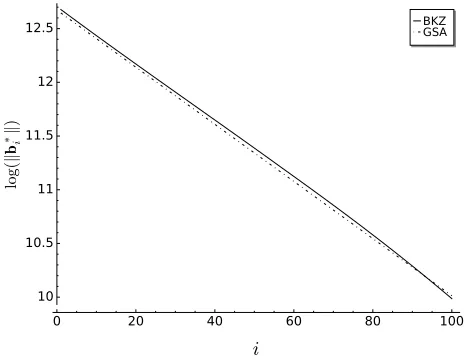
To compare the expected output of BKZ, DBKZ, and Slide reduction, we generated a Goldstein-Mayer lattice [17] in dimension n = 200 with numbers of bit size 2000, applied LLL to it, and simulated the execution of BKZ with block size k = 100 until no more progress was made. The output in terms of the logarithm of the shape of the basis for the first 100 basis vectors is shown in Figure 1 and compared to the GSA. Recall that the latter represents the expected output of DBKZ and, to some degree, Slide reduction. Under the assumption that Heuristic 1 and the BKZ simulator are accurate, one would expect BKZ to behave a little worse than the other two algorithms in terms of output quality.
6
Experiments
For an experimental comparison, we implemented DBKZ and Slide reduction in fpLLL. SVP re-duction in fplll is implemented in the standard way as described in Section 2.1. For dual SVP reduction we used the algorithm explained in the Section 7.
6.1 Methodology
0 20 40 60 80 100 10
10.5 11 11.5 12 12.5
i
lo
g(
k
b
∗ki
)
BKZ GSA
Figure 1: Expected shape of the first 100 basis vectors in dimension n = 200 after BKZ compared to the GSA. Note that the latter corresponds exactly to the expected shape of the first 100 basis vectors after DBKZ (cf. 2).
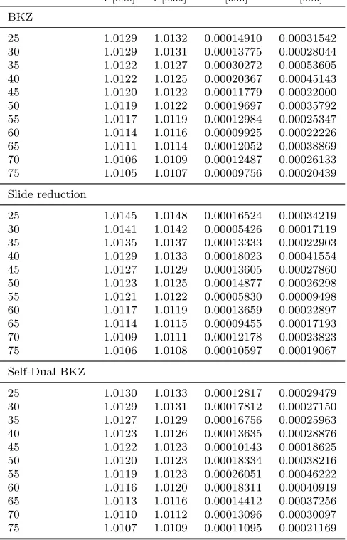
Since experiments with lattice reduction are rather time consuming, it is infeasible to generate as much data as desirable to estimate statistical parameters like the mean value and standard deviation accurately. A standard statistical technique to overcome this is to use bootstrapping to compute confidence intervals for these parameters. Roughly speaking, in order to compute the confidence interval for an estimator from a set ofN samples, we samplelsets of sizeN with replacement from the original samples and compute the estimator for each of them. Intuitively, this should give a sense of the variability of the estimator computed on the samples. Our confidence interval with confidence parameter α, according to the bootstrap percentile interval method, is simply the α/2 and 1−α/2 quantiles. For further discussion we refer to [70]. Throughout this work we useα=.05 and l = 100. The complete confidence intervals for mean value and standard deviation are listed in Appendix B. Whenever we refer to the standard deviation of a distribution resulting from the application of a reduction algorithm and computing the root Hermite factor achieved, we mean the maximum of the corresponding confidence interval.
It is folklore that the output quality of lattice reduction algorithms measured in the root Hermite factor depends mostly on the block size parameter rather than on properties of the input lattice, like the dimension or bit size of the numbers, at least when the lattice dimension and size of the numbers is large enough. A natural approach to comparing the different algorithms would be to fix a number of lattices of certain dimension and bit size and run the different algorithms with varying block size on them. Unfortunately, Slide reduction requires the block size to divide the dimension.9 To circumvent this we select the dimension of the input lattices depending on the block sizes we want to test, i.e. n = t·k, where k is the block size and t is a small integer. This is justified as most lattice attacks involve choosing a suitable sublattice to attack, where such a requirement can easily be taken into account. Since for very small dimensions block reduction performs a little better then in larger dimensions, we need to deal with a trade-off here: on the one hand we need to ensure that the lattice dimensionnis large enough, even for small block sizes, so that the result
9
is not biased positively for small block sizes due to the small dimension. On the other hand, if the lattice dimension grows very large we would have to increase the precision of the GSO computation significantly which would result in an artificial slow down and thus limit the data we are able to collect. Our experiments and previous work [16] suggest that the bias for small dimensions weakens sufficiently as soon as the lattice dimension is larger than 140, so for the lattice dimension n we select the smallest multiple tof the block sizek such thatt·k≥140.
For each block size we generated 10 different subset sum lattices in dimension n in the sense of [19] and we fix the bit size of the numbers to 10·nfollowing previous work [19,36]. Experimental studies [43] have shown that this notion of random lattices is suitable in this context as lattice reduction behaves similarly on them as on “random” lattices in a mathematically more precise sense [17]10. Then we ran each of the three reduction algorithms with corresponding block size on each of those lattices. For BKZ and DBKZ we used the same terminating condition: the algorithms terminate when the slope of the shape of the basis does not improve during 5 loop iterations in a row (this is the default terminating condition in fpLLL’s BKZ routine with auto abort option set). Finally, for sufficiently large block sizes (k >45), we preprocessed the local blocks with BKZ-(k/2) before calling the SVP oracle, since this has been shown to achieve good asymptotic running time [69] and also seemed a good choice in practice in our experiments.
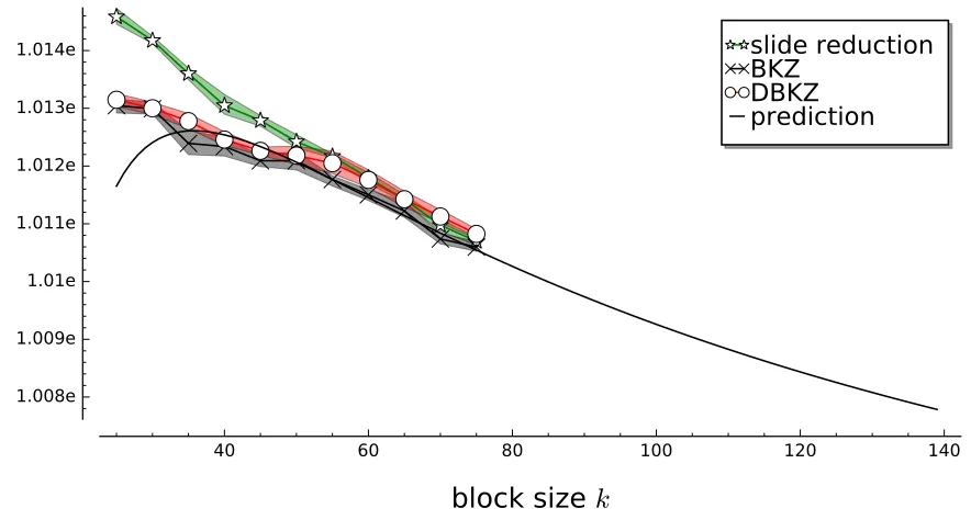
6.2 Results
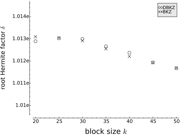
Figure 2 shows the average output quality including the confidence interval produced by each of the three algorithms in comparison with the prediction based on the Gaussian Heuristic (cf. Equation (4)). It demonstrates that BKZ and DBKZ have comparable performance in terms of output quality and clearly outperform Slide reduction for small block sizes (<50), which confirms previous reports [16]. For some of the small block sizes (e.g. k = 35) BKZ seems to perform unexpectedly well in our experiments. To see if this is indeed inherent to the algorithms or a statistical outlier owed to the relatively small number of data points, we ran some more experiments with small block sizes. We report on the results in Appendix A, where we show that the performance of BKZ and DBKZ are actually extremely close for these parameters.
Furthermore, Figure 2 shows that all three algorithms tend towards the prediction given by Equation (4) in larger block sizes, supporting the conjecture, and Slide reduction becomes quite competitive. Even though BKZ still seems to have a slight edge for block size 75, note that the confidence intervals for Slide reduction and BKZ are heavily overlapping here. This is in contrast to the only previous study that involved Slide reduction [16], where Slide reduction was reported to be entirely noncompetitive in practice and thus mainly of theoretical interest.
Figure 3 shows the same data separately for each of the three algorithms including estimated standard deviation. The data does not seem to suggest that one or the other algorithm behaves “nicer” with respect to predictability – the standard deviation ranges between 0.0002 and 0.0004 for all algorithms, but can be as high as 0.00054 (cf. Appendix B). Note that while these numbers might seem small, it affects the base of the exponential that the short vector is measured in, so small changes have a large impact. The standard deviation varies across different block sizes, but there is no evidence that it might converge to smaller values or even 0 in larger block sizes. So we have to assume, that it remains a significant factor for larger block sizes and should be taken into account in cryptanalysis. It is entirely conceivable that the application of a reduction algorithm
10
40
60
80
100
120
140
1.008e
1.009e
1.01e
1.011e
1.012e
1.013e
1.014e
block size
k
root Hermite factor
slide reduction
BKZ
DBKZ
prediction
Figure 2: Confidence interval of average root Hermite factor for random bases as computed by different reduction algorithms and the prediction given by Equation (4).
yields a root Hermite factor significantly smaller than the corresponding mean value.
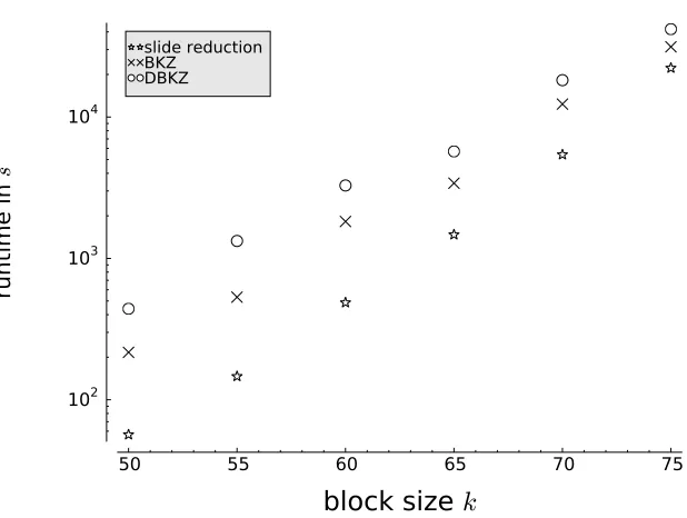
In order to compare the runtime of the algorithms we ran separate experiments, because due to the way we selected the dimension, the data would exhibit a somewhat strange “zigzag” behavior. For each block size 50≤k≤75 we generated again 10 random subset sum lattices with dimension
n= 2k and the bit size of the numbers was fixed to 1400. Figure 4 shows the average runtime for each of the algorithms and block size in log scale. It shows that the runtime of all three algorithms follows a close to single exponential (in the block size) curve. This supports the intuition that the runtime mainly depends on the complexity of the SVP oracle, since we are using an implementation that preprocesses the local blocks before enumeration with large block size. This has been shown to achieve an almost single exponential complexity (up to logarithmic factors in the exponent) [69]. The data also shows that in terms of runtime, Slide reduction outperforms both, BKZ and DBKZ. But again, with increasing block size the runtime of the different algorithms seem to con-verge to each other. Combined with the data from Figure 2 this suggests that all three algorithms offer a similar trade-off between runtime and achieved Hermite factor for large block sizes.
30 40 50 60 70 1.01e
1.011e 1.012e 1.013e 1.014e 1.015e
block size k
root Hermite factor
(a) BKZ
30 40 50 60 70
1.01e 1.011e 1.012e 1.013e 1.014e 1.015e
block size k
root Hermite factor
(b) Slide Reduction
30 40 50 60 70
1.01e 1.011e 1.012e 1.013e 1.014e 1.015e
block size k
root Hermite factor
(c) DBKZ
Figure 3: Same as Figure 2 with estimated standard deviation
50
55
60
65
70
75
10
210
310
4block size
k
ru
nt
im
e i
n
s
slide reduction BKZ
DBKZ
7
Dual Enumeration
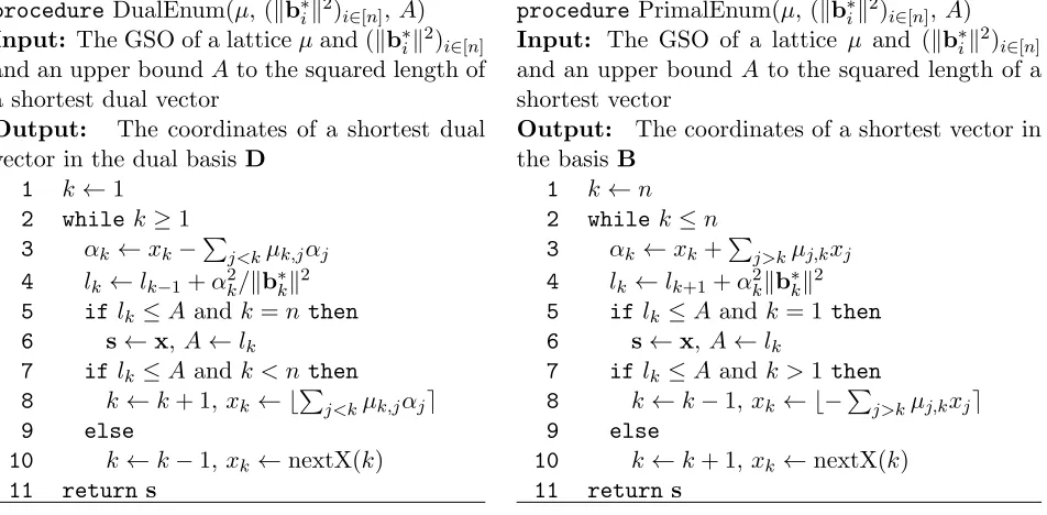
Similar to Slide reduction, DBKZ makes intensive use of dual SVP reduction of projected blocks. The obvious way to achieve this reduction is to compute the dual basis for the projected block, run the primal SVP reduction on it, and finally compute the primal basis of the block. While the transition between primal and dual basis is a polynomial time computation and is thus dominated by the enumeration step, it does involve matrix inversion, which can be quite time consuming in practice. To address this issue, Gama and Nguyen [15] proposed a different strategy. Note that SVP reduction, as performed by enumeration, consists of two steps: (1) the coordinates of a shortest vector in the given basis are computed, and (2) this vector is inserted into the basis. Gama and Nguyen observe that for dual SVP reduction, (2) can be achieved using the coordinates obtained during the dual enumeration by solely operating on the primal basis. Furthermore, note that the enumeration procedure (step (1)) only operates on the GSO of the basis so it is sufficient for (1) to invert the GSO matrices of the projected block, which is considerably easier since they consist of a diagonal and an upper triangular matrix. However, this still incurs a computational overhead of Ω(n3).
We now introduce a way to find the coordinates of a shortest vector in the dual lattice without computing the dual basis or dual GSO. As a warm-up, note that the enumeration procedure applied to the dual basis computes all possible coefficients of short vectors in the dual basis. We can enumerate these coefficients xi =hv,bii ∈Z of the shortest dual vectorv directly and bound the complexity of this approach the following way:
xi =hv,bii=hv,b∗ii − X
j<i
µi,jhv,b∗ji.
Settingx∗j =hv,b∗ji, which we can compute from (x1, . . . , xj), we get
xi+ X
j<i
µi,jx∗j =hv,b∗ii
and so
|xi+ X
j<i
µi,jx∗j| ≤ kvkkb∗ik ≤ ˆ
λ1
kd†ik
which is exactly what one would expect, i.e. it corresponds to the complexity of enumerating all dual lattice points in a parallelepiped. This simple observation suggests that there is an algorithm to compute the coordinates of the shortest dual vector just as efficient as for the shortest primal vector. However, without the dual basis there is no obvious way to evaluate the quality of a solution, i.e. the lengths of a dual vector given only its coordinates in the dual basis. Furthermore, without being able to evaluate partial solution, we can only enumerate in parallelepipeds, while classical enumeration in the primal is able to enumerate lattice points in a sphere by subtracting the length of partial solutions from the enumeration radius. The following Lemma addresses this issue and will result in a dual enumeration algorithm that strongly resembles the primal enumeration routine.
for any k ≤ n, the (uniquely defined) vector w(k) ∈ span(B[1,k]) such that hw(k),bii = xi for all
i≤k, can be expressed as w(k)=P i≤kαib
∗
i/kb∗ik2 where
αi =xi− X
j<i
µi,jαj. (15)
Proof The conditionw(k)∈span(B[1,k]) directly follows from the definition ofw(k)=
P
i≤kαib
∗
i/kb∗ik2. We need to show that this vector also satisfies the scalar product conditionshw(k),bii=xi for all
i≤k. Substituting the expression for w(k) in the scalar product we get
hw(k),bii= X
j≤k
αj
hb∗j,bii kb∗jk2 =
X
j≤i
αj
hb∗j,bii
kb∗jk2 =αi+
X
j<i
αjµi,j =xi
where the last equality follows from the definition of αi. 2
This shows that if we enumerate the levels fromk= 1 ton(note the reverse order as opposed to primal enumeration) we can easily computeαkfrom all the given or previously computed quantities inO(n). The length of w(k) is given by
kw(k)k2 =X i≤k
α2i/kb∗ik2 =kw(k−1)k2+α2
k/kb
∗
kk2. (16)
To obtain an algorithm that is practically as efficient as primal enumeration, it is necessary to apply the same standard optimizations known as SchnorrEuchner enumeration to the dual enumer-ation. It is obvious that we can exploit lattice symmetry and dynamic radius updates in the same fashion as in the primal enumeration. The only optimization that is not entirely obvious is enu-merating the values forxk in order of increasing length of the resulting partial solution. However, from Equation (15) and (16) it is clear that we can start by selectingxk=b
P
j<kµk,jαje in order to minimize the first value ofαk, and then proceed by alternating around this first value just as in the SchnorrEuchner primal enumeration algorithm.
It is also noteworthy that being able to compute partial solutions even allows us to apply pruning [14] directly. In summary this shows that dual SVP enumeration should be just as efficient as primal enumeration. To illustrate this, Algorithm 2 and 3 show the SchnorrEuchner variant of the two enumeration procedures.11
11
Algorithm 2 Dual Enumeration
procedure DualEnum(µ, (kb∗ik2)
i∈[n],A) Input: The GSO of a latticeµand (kb∗ik2)
i∈[n]
and an upper boundAto the squared length of a shortest dual vector
Output: The coordinates of a shortest dual vector in the dual basis D
1 k←1
2 while k≥1
3 αk←xk−Pj<kµk,jαj
4 lk←lk−1+α2k/kb
∗
kk2
5 if lk≤A and k=nthen
6 s←x,A←lk
7 if lk≤A and k < nthen
8 k←k+ 1, xk ← bPj<kµk,jαje
9 else
10 k←k−1,xk ←nextX(k)
11 returns
Algorithm 3 Primal Enumeration
procedure PrimalEnum(µ, (kb∗ik2)
i∈[n],A) Input: The GSO of a lattice µ and (kb∗ik2)
i∈[n]
and an upper bound A to the squared length of a shortest vector
Output: The coordinates of a shortest vector in the basis B
1 k←n
2 whilek≤n
3 αk←xk+Pj>kµj,kxj
4 lk ←lk+1+α2kkb
∗
kk2
5 iflk≤Aand k= 1 then
6 s←x,A←lk
7 iflk≤Aand k >1 then
8 k←k−1,xk← b−Pj>kµj,kxje
9 else
10 k←k+ 1,xk←nextX(k)
11 returns
Implementation Notes To give some experimental evidence that the dual enumeration is just as efficient as primal enumeration, we implemented it in fpLLL.12 Note that Algorithm 2 can be easily added to an implementation of Algorithm 3 by using special cases in data accesses and a few operations. Furthermore, in order to avoid the division in line 4 we precomputed the values 1/kb∗kk2 for all k. We compared the implementation with the primal enumeration on 10 random
bases (in the same sense as in Section 6) in dimension 35 ≤ n ≤ 50. As expected, the rate of enumeration was close to equal in both cases – around 3.2·107 nodes per second (cf. Table1), which
corresponds to slightly more than 100 cycles per node on our 3.4 Ghz test machine. The slight discrepancies (and the low rate forn= 35) can be explained by the variable number of nodes that were enumerated and thus certain setup costs are amortized over a different number of nodes.
n 35 40 45 50
primal 2.73 3.16 3.13 3.17
dual 2.77 3.19 3.18 3.27
Table 1: Rate of enumeration (in 107 nodes pers) in primal and dual enumeration
Inserting the Shortest Dual Vector For completeness we briefly review how to insert the shortest dual vector into the dual basis using its coordinates in the dual basis and operating solely on the primal basis. Let vbe a shortest dual vector. Its coefficients in the dual basis are given by
x=BTv∈Zn. Our goal is to transformB into a basisB¯ of the same lattice such thatB¯Tv=e n,
12At the point of publication of this work, a modified version of this implementation is now included in the main
whereenis then-th vector of the standard basis (which is equivalent tov being then-th vector of the dual of B¯). This can be achieved by computing a unimodular matrix U such that Ux =en, for example by computing the GCD of the non zero coefficients of x (which must be 1 since v
is a shortest dual vector). Then we have en = Ux = UBTv and so with B¯ = BUT, we obtain
en=B¯Tv as desired. Note that we do not need to knowv in order to achieve this – knowing xis sufficient.
It is not immediately clear that the size of the numbers during the execution of this step is polynomially bounded. However, Gama and Nguyen [15] show that it is if using the right strategy for the GCD computation and we will skip this detail here.
8
Conclusion and Future Work
While our experimental study of lattice reduction confirms that the average root Hermite factor achieved by lattice reduction is indeed, as conjectured, given by Equation (4), the standard deviation is large enough that it is conceivable that asingle instance finds a much shorter vector. This means that cryptanalytic estimates should take this into account. Unfortunately, it is at this point unclear how to apply our results to cryptanalysis. Before being able to make meaningful security estimates, there are two issues to solve.
On the one hand, since we usually want to estimate the attack complexity for instances much too hard to solve in practice, we need a way to predict the standard deviation in a similar way as the average root Hermite factor. Given our results (cf. Figure 3), we believe it might be reasonable to assume that the standard deviation is upper bounded by a constant, e.g. σ= 0.0006, but more work is needed to verify this assumption.
Once we can predict (in a conservative and meaningful way) the mean value and standard deviation of the underlying distribution of the root Hermite factor achieved by lattice reduction, we need to find a way to translate this to a root Hermite factor that is unlikely to be achieved by lattice reduction. Since we do not know the underlying distribution, bounds like Chebyshev’s inequality spring to mind. Unfortunately, bounds that make no or very weak assumptions on the underlying distribution are generally very poor and thus would lead to overly conservative estimates. For example, Equation (4) estimates the mean root Hermite factor achieved by lattice reduction with block size k = 100 to be δ100 = 1.00926. If we use Chebyshev’s inequality to estimate ¯δ100
such that an attacker running BKZ-100 (which is by no means unrealistic) has a probability of less than 1% (which is actually still quite large) to achieve a root Hermite factor less than ¯δ100, we
would need to set ¯δ100 = 1.00926−10·σ = 1.00326. This is clearly unrealistic – a root Hermite
factor of 1.005 is still believed to be completely out of reach today and our results give no reason to believe otherwise.
With our new dual enumeration algorithm we provide another tool to practically examine dif-ferent reduction algorithms. This should facilitate experimental research into reduction algorithms that make use of dual SVP reduction, like variants of Slide reduction. Future lines of research could explore if, for example, the block Rankin reduction algorithm of [28] can be efficiently implemented by using it to apply the densest sublattice algorithm of [10] to the dual lattice. This could be used to achieve potentially stronger notions of reduction with better output quality.
Acknowledgment
We thank Arnold Neumaier for completing the analysis of the convergence of DBKZ. Furthermore, we thank Arnold and the anonymous reviewers of the Eurocrypt 2016 committee for many helpful comments on a previous version of this work. We also thank Florian G¨opfert for helpful discussions in the early stages of the development of the dual enumeration algorithm.
References
[1] M. Ajtai. Generating hard instances of lattice problems. Complexity of Computations and Proofs, Quaderni di Matematica, 13:1–32, 2004. Preliminary version in STOC 1996.
[2] M. Ajtai and C. Dwork. A public-key cryptosystem with worst-case/average-case equivalence. InProceedings of STOC ’97, pages 284–293. ACM, May 1997.
[3] A. Akhavi and D. Stehl´e. Speeding-up lattice reduction with random projections (extended abstract). In E. S. Laber, C. F. Bornstein, L. T. Nogueira, and L. Faria, editors, LATIN, volume 4957 ofLecture Notes in Computer Science, pages 293–305. Springer, 2008.
[4] M. Albrecht, D. Cad´e, X. Pujol, and D. Stehl´e. fplll-4.0, a floating-point LLL implementation. Available athttp://perso.ens-lyon.fr/damien.stehle.
[5] M. R. Albrecht, R. Player, and S. Scott. On the concrete hardness of learning with errors. Cryptology ePrint Archive, Report 2015/046, 2015. http://eprint.iacr.org/.
[6] A. Bachem and R. Kannan. Lattices and basis reduction algorithm. Technical Report 84-006, Mathematisches Institut, Universit¨at zu K¨oln, 1984.
[7] Y. Chen. R´eduction de r´eseau et s´ecurit´e concr`ete du chiffrement compl`etement homomorphe. PhD thesis, ENS, Paris, 2013. Thse de doctorat dirige par Nguyen, Phong-Quang Informatique Paris 7 2013.
[8] Y. Chen and P. Q. Nguyen. BKZ 2.0: Better lattice security estimates. In ASIACRYPT, volume 7073 ofLecture Notes in Computer Science, pages 1–20. Springer, 2011.
[9] C. Coup´e, P. Nguyen, and J. Stern. The effectiveness of lattice attacks against low-exponent RSA. InProc. of PKC ’99, number 1560 in LNCS, pages 204–218. Springer, Berlin Germany, Mar. 1999.