An Approach For Modification Of Block Match Three Dimension De-Noising Algorithm With Pre-Filtering In Nonlocal Domain

(1)

An Approach for Modification of Block Match Three

Dimension De-Noising Algorithm with Pre-Filtering In

Nonlocal Domain

Kamalakshi NP 1#

P

, ,Dr M N ShanmukhaswamyP 2

P

1

P

Research Scholar JSSRF,Mysore ,UOM

#Dept of Computer Science &Engg Sapthagiri College of Engg ,Bangalore VTU,Belagaum,India

P

2

P

Professor and Head Dept of Electronics & Communication SJCE Mysore , India

P

1

P

[email protected], , 32TP 2

PU

[email protected]U32T

Abstract.BM3D (Block Matching three dimension)is one of the popular de-noising state of art algorithm which works on transform domain .It has lot of engineering in it. Even though BM3D outperforms all other de-noising algorithms, the performance degrades as sigma value increases ,also some artifacts are introduced as the noise level increases. To overcome this drawbacks a new modified approach is proposed by adding an additional step for pre-filtering & removing noise by edge detection. Experimental results depicts that proposed approach gives better results in terms of PSNR (Peak signal to Noise Ratio) and visual quality with a reasonable computational burden

Keywords:

1. Introduction

Image processing is a very renowned area of research. But the de-noising is quite a old area of interest which has lot of real time application. With the advent of various technology and well equipped devices for capturing an image but some noise is introduced always and de-noising which is a preprocessing step is one of the challenging task in the area of image processing. Vast Literature exists which depicts emerging work in the de-noising so depends on some assumptions about the removal of random noise.

Presently, patch based de-noising image processing has become very eminent using which a local patches (Patch(block or Fragment ):is a sub-image of an image of size NxN) has been adopted by most of the researchers and hence very popular due to its highly effective .Taking advantage of the redundancy of small sub-images inside the image of interest. The core idea behind these and many other contributions is the same, for given the image to be processed, extract all possible patches with overlaps; these patches are very minute compared to the image size (a typical patch size would be 8 × 8 pixels). The processing takes by operating on these patches and furnishing interrelations between them. The final image is formed by the modification of patches (or sometimes only their center pixels) and later put them back into the original position . The paper is organized as section II discuss about related work, section III about proposed work and section IV about the results & Discussion & Finally conclusion

(2)

IJISET - International Journal of Innovative Science, Engineering & Technology, Vol. 2 Issue 12, December 2015. www.ijiset.com

ISSN 2348 – 7968

2. Related Work

BM3D is currently known as the state of the art method for image de-noising and outperforms all other algorithm when it comes to de-noise AWGN at a reasonable computational cost[1]. BM3D depends on the presumption that an image has a locally sparse representation in the transform domain. In BM3D the sparsity is enhanced by grouping similar 2D fragments into 3D data array which the authors called “groups”. Because each block in the group was chosen according to some similarity measure with respect to a reference block, the use of a higher dimensional filtering of each group was possible. This exploits the potential similarity between grouped blocks to estimate the true signal in each of them by producing a highly sparse representation in 3D transform domain, so that the noise can be removed by wavelet shrinkage. This approach of exploiting similarity and estimating the original signal is called as collaborative filtering.

Issues in BM3D

BM3D has few lacunae and modification are still possible, especially for higher noise levels. BM3D introduces many artifacts when the noise level is high (sigma>40 ). The performance of noise reduction also significantly drops as the noise level increases. When the noise level is large, block matching is not reliable any more, as blocks which are not similar to the referenced block can easily be grouped together into the 3D array, resulting in less sparser representation in transform domain. It also tends to give poor visual results when exposed to micro-textured zones in natural images. Another important drawback of BM3D is that it blurs sharp edges, as it uses a weighted averaging at the end of each step (i.e. first step and second step), which works more like a low pass filter. BM3D also reduces the contrast of images which can easily be observed in almost all of its denoised images.Also, if the image is highly contaminated by noise, the image features becomes inseparable from the noise itself. In these situations, though it preserves the fine image details after denoising, it can blur the edges after the collaborative filtering and aggregation step I..In the transform domain the edges and the noises are not distinguishable and this forces the filtering process to remove some of the edge information making edges blurry.

3. Proposed Algorithm

The unique feature of this algorithm compared to BM3D is that it does a pre-filtering that is the first step where in it identifies whether a pixel is corrupted or no and the remaining two steps are similar to BM3D. The algorithm consists of three steps

Step1: Identifying a noisy pixel (based on current pixel & its neighborhood values)

Step 2: To determine the basic estimate

Step 3: Estimation of the true image from the basic estimate and the noisy image

(3)

IV Noise Mathematical Model

Assume a noise model with true image y being corrupted by AWGN as

z (x) = y (x) + η (x) , x ε X (1)

where x denotes a 2D index or location or spatial coordinate belonging to the image

domain X ⊂ ZP

2

P

, y is the true image, and is i.i.d. zero-mean Gaussian noise with variance (0, 𝜎2P

).

Modified BM3D Proposed Algorithm

The algorithm consists of three steps

Step1: Identifying a noisy pixel (based on current pixel & its neighborhood values)

a. Usea sliding window to identify the noisy pixel and restore it

b. Apply a median filter to reduce the noisy pixels from image before applying the

actual denoising method

c. Designate current pixels as Px. Compare each pixel with its neighboring pixels

d. If Px is corrupted

i. Px value is maximum or minimum of all other pixel values in the

corresponding neighbor

ii. Sort the pixel value except Px of the filter window w_x,n in ascending order

iii. s(x)=(s1(x),s2(x)…..s8(x))

∂� (x) = �1, {P𝑥 < 𝑚𝑖𝑛 {𝑠(x)} −τpre }V{P𝑥 ≥ �max{s(x)} −τpre�}

0, otherwise (2)

Where τ_pre is a threshold value

if(∂� (x) = 1)

then apply median filter on the window w_x,n to determine the value of the pixel

and restore it

med� f (x) = �s(x) ∈ wx,

n_{, s(x) ≠ px}, if ∂ (x) = 1}

Px, otherwise (3)

else restore the original pixel

Step 2: To determine the basic estimate

Here, we get the basic estimate using the pre-filtered version of the noisy image. We follow the following procedure for two different block sizes of , and depending on the noise

level present in the examined image.

i) To identify the patches similar to the reference patch or noise standard deviation crosses 39

denoising performance has a sharp drop. To overcome this issue, it is advised to use coarse prefiltering to measure the block-distance. This prefiltering is realized by applying a normalized 2-D linear transform on both blocks and then hard-thresholding the obtained coefficients, which results in

(4)

ISSN 2348 – 7968

𝑑�𝑍_𝑥𝑅,𝑍_𝑥� =||𝛾

′_{� 𝜏}

2𝐷

ℎ𝑡_{(𝑍𝑥𝑅)�−𝛾}′_{� 𝜏}

2𝐷 ℎ𝑡_{(𝑍𝑥)�||}

2 2

(𝑁1ℎ𝑡2)

(4)

where 𝛾′ is a hard threshold operator and 𝜏_2𝐷ℎ𝑡 is a 2-D linear unitary transform operator. Each

group is made by stacking together maximum 𝑁₁ℎ𝑡2 similar noisy blocks, with similarity

distances less than a predefined threshold 𝜏_{𝑚𝑎𝑡𝑐ℎ}ℎ𝑡 match in a 3-D array form, R To stack

the similar patches to form a 3D group

𝑆_𝑥𝑅ℎ𝑡 = {𝑥 ∈ 𝑋 ∶ 𝑑(𝑍_𝑥𝑅, 𝑍_𝑥) ≤ 𝜏_{𝑚𝑎𝑡𝑐ℎ}ℎ𝑡 (5)

Using the d-distance (4) is a set 𝑆_𝑥𝑅ℎ𝑡 which contains the coordinates of blocks similar to 𝑍_𝑥𝑅,

𝜏𝑚𝑎𝑡𝑐ℎℎ𝑡 is the maximum for which two blocks are similar

ii) An effective collaborative filtering can be asumed as shrinkage in transform domain.

Suppose d+1-dimension groups of similar signal fragments are already grouped, the collaborative shrinkage comprises of the following steps.

• For each group Introduce a d+1-dimensional linear transform.

• To attenuate noise shrink (by hard-thresholding in step 1| Wiener filtering in step

2) the transform coefficients

• To get estimates of all grouped fragments invert the linear transform to produce.

iii) Three dimension Transform of a group is done by hard thresholding of the transform

coefficients, then inverse the transform and return the estimates of the block to their original positions

𝑌�_𝑠

𝑥𝑅ℎ𝑡

ℎ𝑡 _{= 𝜏}

3𝐷ℎ𝑡 −1( 𝛾(𝜏3𝐷ℎ𝑡 �𝑍𝑠_𝑥𝑅ℎ𝑡�) ) (6)

𝛾(𝑥) = �0 , 𝑖𝑓|𝑥| ≤ 𝜆3𝐷ℎ𝑎𝑟𝑑

𝑥 , 𝑜𝑡ℎ𝑒𝑟𝑤𝑖𝑠𝑒 𝜎 } (7)

iv) Use weighted average of all the obtained overlapping estimates to obtain the basic

estimate of the image

𝜔𝑋ℎ𝑡 = � 1 𝜎2_𝑁

ℎ𝑎𝑡𝑋𝑅 , 𝑖𝑓𝑁ℎ𝑎𝑡

𝑋𝑅 _{≥ 1}

1, 𝑜𝑡ℎ𝑒𝑟𝑤𝑖𝑠𝑒 (8)

Once the 3D block is done collaborative filtering of 𝑍𝑠_𝑥𝑅ℎ𝑡 (N1xN1x| 𝑆_𝑥𝑅ℎ𝑡),estimate aggregation

After processing all reference blocks, we have a set of local block estimates 𝑌�_𝑠

𝑥𝑅ℎ𝑡

ℎ𝑡_{, ;x}

RRR∈ X (and

their corresponding weights SRxRR, ;xRRR∈ X), which forms an overcomplete representation of the

estimated image due to the overlap between the blocks. The final estimate is given by

(5)

𝑌�𝑏𝑎𝑠𝑖𝑐_{(𝑥) =}∑ ∑ 𝜔𝑋𝑅 ℎ𝑡_𝑌

𝑋𝑚ℎ𝑡 𝑋𝑅(𝑋) 𝑥𝑚∈𝑆_𝑋𝑅ℎ𝑡

𝑋𝑅∈𝑋

∑ ∑ 𝜔_𝑋𝑅ℎ𝑡_𝒳

𝑋𝑚(𝑋) 𝑥𝑚∈𝑆_𝑋𝑅ℎ𝑡

𝑋𝑅∈𝑋

, ∀𝑥∈ 𝑋 … … … . (9)

Edge map building

For the the preliminary basic estimation apply the Canny edge detector to build a edge map. The Canny edge detector prominent the regions with high spatial derivatives by applying a Gaussian smoothing with a kernel size to reduce the level of noise in the input image, followed by the processing of derivative in both x and y direction to get the magnitude and direction of gradient,

𝑑 = �(𝐷2

𝑥 (𝑥, 𝑦) + �𝐷2𝑦 (𝑥, 𝑦� (11)

Magnitude

𝜃 = arctan (𝐷𝑥

𝐷𝑦) (12)

where D is the magnitude of gradient and θ is angle of gradient. Given the values of the gradient, the algorithm applies non-maximum suppression, which suppresses any pixel that is not at the maximum. This is done by preserving all local maxima in the gradient image, and deleting everything else. Furthermore, the gradient array is reduced by hysteresis that uses two thresholds, and , determined empirically. Pixels with gradient magnitude are discarded, while pixels with gradient magnitude are kept as edges. If the magnitude is between the thresholds (i.e. ), it is only kept as an edge if and only if there is a path from this pixel to a pixel with gradient Once we get the edge map by applying the Canny, we binarize the array values, where, represents the Canny edge detection process and represents the binarization method. The obtained edge guide is then used to combine the values from the two preliminary basic estimates and to form the final basic estimate. This is done by processing each pixel in a raster scan fashion and obtaining the edge strength for that location based on its neighboring pixels.

The PDF of noisy (ZRxR,Zx) ,are likely to overlap heavily and this results in error grouping

ie., blocks with greater distances than the threshold are matched as similar, where as blocks with smaller distances are left out.

Step 3: Estimation of the the true image from the basic estimate and the noisy image

 The third step is similar to the original BM3D algorithm except instead of original

noisy image we use the pre-filtered image as the input to this step.

 In this step, both the basic estimate and the pre-filtered noisy image are used to improve

the denoising.

(6)

ISSN 2348 – 7968

 We take advantage of the basic estimate by processing the grouping within the

basic estimate and using collaborative Wiener filtering.

 The significant reduction of noise in the basic estimate allows us to use the normalized

distance for grouping the similar blocks for reference blocks

Find out the locations of the blocks close to the reference one by block matching in the basic estimate. From the obtained locations, form two 3D groups which are from the noisy image and the basic estimate.

𝑆_𝑋𝑅𝑤𝑖𝑒 = �𝑥 ∈ 𝑋:|�𝑌�𝑋𝑅

𝑏𝑎𝑠𝑖𝑐_−𝑌 𝑋 �_𝑅𝑏𝑎𝑠𝑖𝑐|�

2 2

(𝑁1𝑤𝑖𝑒)2 ≤𝜏𝑚𝑎𝑡𝑐ℎ

𝑤𝑖𝑒 _{} (}₁₂₎

Perform 3D transform to both the groups. And later perform wiener filtering on the noisy one with the energy spectrum of the basic estimate. The 3D transform domain collaborative Weiner

filtering is done by element by element multiplication of Weiner shrinkage coefficient 𝑊_𝑆

𝑋𝑅𝑤𝑖𝑒

and the 3D transform domain coefficients of noisy data 𝑇_3𝐷𝑤𝑖𝑒(𝑍_𝑠

𝑥𝑅 𝑤𝑖𝑒)

𝑊_𝑆 𝑋𝑅𝑤𝑖𝑒 =

|𝑇_3𝐷𝑤𝑖𝑒 (𝑌� 𝑆𝑋𝑅𝑏𝑎𝑠𝑖𝑐𝑤𝑖𝑒 )|2 |𝑇_3𝐷𝑤𝑖𝑒 (𝑌�

𝑆𝑋𝑅𝑏𝑎𝑠𝑖𝑐𝑤𝑖𝑒 )|2+𝜎2

(13)

The 3D array 𝑌�_𝑆

𝑋𝑅𝑤𝑖𝑒

𝑤𝑖𝑒_{is made of the block estimates}_𝑌�

𝑥𝑤𝑖𝑒,𝑥𝑅, SVx S ∈ 𝑆𝑋

𝑅

𝑤𝑖𝑒

𝑌�_𝑆 𝑋𝑅𝑤𝑖𝑒=

𝑤𝑖𝑒 _𝑇

3𝐷𝑤𝑖𝑒−1(𝑊𝑆_𝑥𝑅𝑤𝑖𝑒(𝑇3𝐷𝑤𝑖𝑒(𝑍𝑠_𝑥𝑅𝑤𝑖𝑒)) (14)

The aggregration of the block wise estimate weights are computed as follows

𝜔𝑥𝑅𝑤𝑖𝑒 = 𝜎−2| �𝑊𝑆_𝑥𝑅𝑤𝑖𝑒� |2−2 (15)

The final estimate after wiener filtering is as follows

𝑌�𝑓𝑖𝑛𝑎𝑙_{(𝑥) =}∑ ∑ 𝜔𝑋𝑅

𝑤𝑖𝑒_𝑌 𝑋𝑚

𝑤𝑖𝑒𝑋𝑅_(𝑋) 𝑥𝑚∈𝑆_𝑋𝑅𝑤𝑖𝑒

𝑋𝑅∈𝑋

∑ ∑ 𝜔_𝑋𝑅𝑤𝑖𝑒_𝒳

𝑋𝑚(𝑋) 𝑥𝑚∈𝑆_𝑋𝑅𝑤𝑖𝑒

𝑋𝑅∈𝑋 , ∀𝑥

∈ 𝑋 (16)

This is the new algorithm devised by modifying BM3D.

4. Results & Discussion

This section is contributed to the performance evaluation of proposed method. The experiments were conducted on images such as Barbara, Pepper , house,Lena, cameraman and compared with original BM3D[02], KSVD[09], NLMeans[08] &NLBayes[10].The metrics used

(7)

for the performance evaluation is PSNR The analysis was done for images with noise levels (i.e. ) 5 to 100. Results presented here are acquired on exactly the same noisy image for both the BM3D and our proposed method. All of our images are 8-bit gray scale images and of dimension 512x512 , except House and Cameraman images, which have 256x256 pixels

The result obtained from the experiments proves that our proposed method shows better result than BM3D in most of images. The PSNR improvement is well for higher noise levels. During subjective evaluation we have shown that the images de-noised by our proposed method preserves edges and details in better manner .In terms of PSNR, our method demonstrates the best performance and outperforms other 4 methods in almost all noise levels for less textured images except in few cases. In particular, the addition of pre-filtering step produce PSNR values almost more than one decibel higher than the original BM3D algorithm for few sigma value..The results (PSNR in db )are tabulated in the following tables for different images

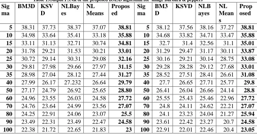
Table 1:Output PSNR of the proposed BM3D algorithm for image Barbara & peppers

Sig ma

BM3D KSV D NLBay es NL Means Propos ed Sig ma BM3 D

KSVD NLB ayes NL Mean s Prop osed

5 38.31 37.73 38.37 37.07 38.81 5 38.12 37.56 38.16 37.27 38.81

10 34.98 33.64 35.41 33.18 35.88 10 34.68 33.82 34.71 33.47 35.88

15 33.11 31.13 32.71 30.74 34.81 15 32.7 31.4 32.56 31.1 35.01

20 31.78 29.21 31.53 30.21 33.01 20 31.29 29.47 31.17 30.11 33.87

25 30.72 29.14 30.31 29.08 32.16 25 30.16 29.21 30.14 28.75 33.08

30 29.81 27.98 29.66 27.97 31.15 30 29.28 28.28 29.12 27.68 33.01

35 28.98 27.04 28.12 27.44 31.27 35 28.52 27.51 28.41 26.61 31.08

40 27.99 26.17 27.232 26.64 29.79 40 27.7 26.65 27.71 25.77 29.8

50 27.17 24.79 26.92 25.65 28.80 50 26.41 26.04 26.66 24.14 28.8

60 24.96 23.55 26.03 24.58 27.72 60 25.55 25.43 25.46 22.96 27.72

70 24.76 23.64 24.99 23.56 27.07 70 24.8 24.11 24.62 22.21 27.07

80 24.25 22.91 24.06 23.07 25.5 80 24.1 23.23 24.04 21.27 25.94

90 23.49 22.31 23.49 22.47 24.58 90 23.61 22.42 23.27 20.7 24.58

100 22.38 21.72 22.65 21.83 23 100 22.91 22.01 22.46 20.4 23.05

The table 1 depicts that PSNR of the proposed method outperformance all other method for image Barbara & pepper

Table 2:Output PSNR of the proposed BM3D algorithm for image House & cameraman

Sig ma

BM3D KSV D NLB ayes NL Mean s Propo sed Sig ma BM3 D KSV D NLB ayes NL Means Propo sed

5 39.83 38.93 39.55 38.69 38.9 5 39.83 38.93 39.55 38.69 38.9

10 36.71 34.9 36.2 34.98 35.88 10 36.71 34.9 36.2 34.98 35.88

15 34.94 32.47 34.35 32.83 34.89 15 34.94 32.47 34.35 32.83 34.89

20 33.77 30.43 33.3 32.3 34.01 20 33.77 30.43 33.3 32.3 33

25 32.86 31.07 33.49 31.24 33.1 25 32.86 31.07 33.49 31.24 33.1

30 32.09 30 31.78 30.3 32.7 30 32.09 30 31.78 30.3 32.7

(8)

ISSN 2348 – 7968

35 31.38 28.82 31.1 29.78 31.12 35 31.38 28.82 31.1 29.78 31.12 40 30.65 28.01 30.37 28.69 29.8 40 30.65 28.01 30.37 28.69 29.8 50 29.69 26.53 29.13 27.44 29.4 50 29.69 26.53 29.13 27.44 29.4 60 28.74 25.07 28.23 26.1 27.7 60 28.74 25.07 28.23 26.1 28.7 70 27.51 25.65 26.95 25.13 27.01 70 27.51 25.65 26.95 25.13 27.01 80 27.16 24.6 26.51 24.37 25.5 80 27.16 24.6 26.51 24.37 25.5 90 26.48 23.94 25.99 23.8 24.58 90 26.48 23.94 25.99 23.8 25 100 25.87 23.07 25.12 23.1 23.75 100 25.87 23.07 25.12 23.1 24.75

The table 2 depicts that PSNR of the proposed method is higher for few sigma values and lesser than BM3D and NLBayes

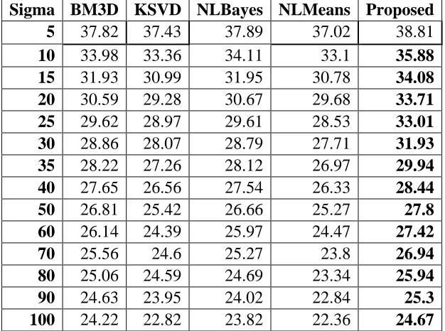
Table 3:Output PSNR of the proposed BM3D algorithm for image Lena

Sigma BM3D KSVD NLBayes NLMeans Proposed

5 37.82 37.43 37.89 37.02 38.81

10 33.98 33.36 34.11 33.1 35.88

15 31.93 30.99 31.95 30.78 34.08

20 30.59 29.28 30.67 29.68 33.71

25 29.62 28.97 29.61 28.53 33.01

30 28.86 28.07 28.79 27.71 31.93

35 28.22 27.26 28.12 26.97 29.94

40 27.65 26.56 27.54 26.33 28.44

50 26.81 25.42 26.66 25.27 27.8

60 26.14 24.39 25.97 24.47 27.42

70 25.56 24.6 25.27 23.8 26.94

80 25.06 24.59 24.69 23.34 25.94

90 24.63 23.95 24.02 22.84 25.3

100 24.22 22.82 23.82 22.36 24.67

The table 3 depicts that PSNR of the proposed method is higher for few sigma values and lesser than BM3D a and NLBayes for image lena

(9)

Figure 1:Comparison of BM3D,KSVD,NLBayes,NLMeans and Proposed method for Barbara Image

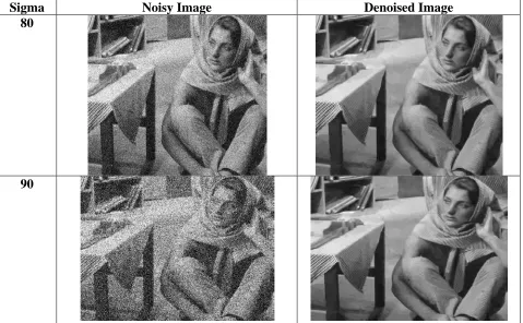
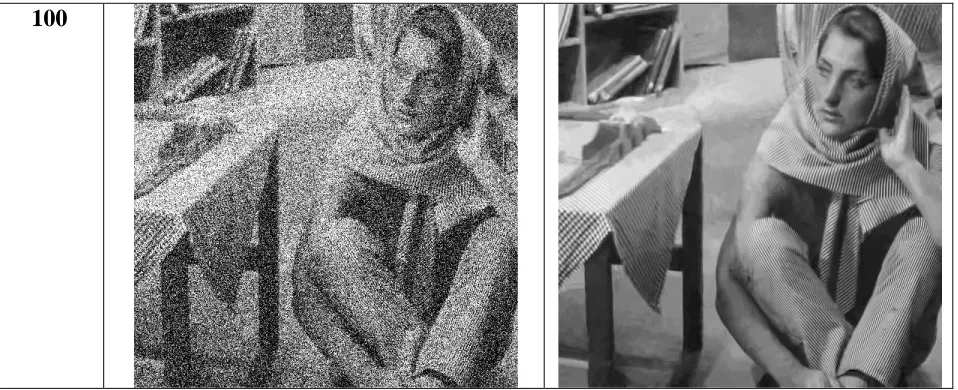
Table 3Noisy & Denoised Image of Barabara for Sigma80,90 & 100

Sigma Noisy Image Denoised Image 80

90

0 10 20 30 40 50 60 70 80 90 100 20

22 24 26 28 30 32 34 36 38 40

Sigma

P

S

NR i

n

d

B

Barbara

BM3D KSVD NL Bayes NLMeans Proposed

(10)

ISSN 2348 – 7968

100

Computational Time:The BM3D ,NLBayes, NLMeans and KSVD algorithms were taken & demonstrated from Image Processing Online on Intel Core(I3) CPU 2.13 MHz RAM 3.GB as in

table 4

Table 5:Computational Time in seconds of BM3D ,KSVD ,NLMeans, NLBayes & Proposed Method

From the above table it can be seen that proposed method imposes computational burden

compared all other methods except for Barbara image due to the addition of pre-filtering step in

the algorithm.

Images Sigma BM3D KSVD NLMeans NLBayes Proposed

Barbara 100 4.92 10.45 14.66 1.62 6.6

Peppers 100 2.12 3.02 3.54 1.02 6.2

Lena 100 4.83 11.34 15.46 2.12 6.1

House 100 2.02 2.42 4.35 1.02 5.8

Cameraman 100 2.02 2.72 3.74 1.22 4.81

(11)

Conclusion

From the experimental results it is found that the proposed method outperforms the state

of art algorithm in terms of objective & subjective visual quality for AGWN noise with

Reasonable computational cost compared to BM3D that is due to additional pre-filtering step at

initial stage

References

1.A. Buades, B. Coll, and J. M. Morel, .A review of image denoising algorithms, with a new Multiscale

Modeling and Simulation, vol. 4, no. 2, pp. 490.530, 2005.

2. K. Dabov, A. Foi, V. Katkovnik, and K. Egiazarian, .Image denoising by sparse 3D transform-domain collaborative filtering ,. IEEE Trans. Image Process., vol. 16, no. 8, pp. 2080.2095, August 2007. 3. M.C. Motwani, M.C. Gadiya and R.C. Motwani, "Survey of Image Denoising Techniques", proceedings of GSPx, Santa Clara, CA., Sep., 2004.

4. A. Buades, B. Coll, and J Morel. On image denoising methods. Technical Report 2004-15, CMLA, 2004.

5.A. Buades, B. Coll, and J Morel. A non-local algorithm for image denoising. IEEE International Conference on Computer Vision and Pattern Recognition, 2005.

6.MLEBRUN,0T0TAn Analysis and Implementation of the BM3D Image Denoising Method,0T0T32TImage Processing

On Line32T,0T0T32T232T (2012), pp. 175–213.0T0T32Thttp://dx.doi.org/10.5201/ipol.2012.l-bm3d32T

7. Antoni Buades, Bartomeu Coll and Jean Michel Morel “An Implementation of Non Local (NL Bayes) Image denoising algorithm “IPOL 2011 pp 1-42 http://dx.doi.org/10.5201/ipol.2011.16

8.Marc Lebrun, Arthur Leclaire “An Implementation and Detailed Analysis of the K-SVD Image Denoising Algorithm “ IPOL 2012 pp. 175–213.0T0T32Thttp://dx.doi.org/10.5201/ipol.2012.l-bm3d32T

9.Antoni Buades, Bartomeu Coll and Jean Michel Morel “Implementation of Non Local Bayes”(NL Bayes) Image denoising algorithm IPOL 2013 pp 1-42 http://dx.doi.org/10.5201/ipol.2013.16