Comparative Study of Machine Learning Models in
Protein Structure Prediction
*Sonal Mishra
1, *Anamika Ahirwar
2*1
Computer Science and Engineering Department, Maharana Pratap College of technology Gwalior. Putli Ghar Road, Near Collectorate, Gwalior-474006, Madhya Pradesh, India
*2Computer Science and Engineering Department, Maharana Pratap College of technology Gwalior.
Abstract -As physical and chemical properties of protein guide to determine quality of the protein structure, it has been used rigorously to distinguish native or native like structure from other predicted structures. In this work, by using six physical and chemical properties we explore the machine learning models and the properties are total empirical energy, secondary structure penalty, total surface area, pair number, residue length and Euclidean distance to predict the RMSD (Root Mean Square Deviation) of a protein structure in the absence of its true native state. There are total 1056 modelled decoys structure having 3078 native structures. The Real Coded Genetic Algorithm (RCGA) is used to determine feature importance and robustness is measured by the K-fold validation of the best predictive model.
The experiments results shows that the random forest model outperforms the other machine learning approaches in RMSD prediction. This work achieved the prediction of RMSD faster and inexpensive.
Keywords—Protein structure prediction, Machine learning, Random forest, RCGA.
Results: The performance result shows that in the prediction of RMSD, the RMSE (Root Mean Square Error) is 0.48; correlation is 0.90; R2 is 0.82; and accuracy is 97.02% (with ± 2 error) respectively on the testing data.
1 INTRODUCTION
for carrying out several biological functions Protein sequences are translated into 3D tertiary forms. Prediction of high resolution protein structure has become one of the “biggest problems“ in modern biology. Physical and Chemical properties of amino acids and their solvent environment are the key determinants in folding a protein sequence into its unique tertiary structure. These factors essentially generate various types of energy contributors such as electrostatic, van der Waals, salvation/desolvation, which create folding pathways.
ab initio approaches for structure determination employ these physical and chemical factors to generate a structure or an ensemble of structures from the sequence as plausible candidates for the native. In an alternative approach, called homology modeling, one uses experimentally known protein structures as templates based on sequence similarity. Because of the insufficient experimental data and lack of knowledge about the true folding path way of proteins to the native ,may
prediction models generate low quality structures .These low quality structures might be look similar to high resolution structure having all the quality assessment criteria but in reality they could be 10-15 °A away from their true native states (Fig. 1). It would be highly desirable to have a predictive model, which can tell how far a structure is from the native in the absence of its experimental structure.
and names Decision Tree, random forest, Linear model and Neural Network for the prediction of RMSD protein structure. By the whole experiments, it is observed that random forest model outperforms the other machine learning approaches in prediction of RMSD. Further, K-fold cross validation is used to measure the robustness of the best predictive model. Finally, for the benchmarking of model correctness, the performance of best predictive model is compared with top-performing ProQ2 (Ray et al., 2012) . The benchmark
method is single model method. ProQ2 is based on Support Vector Machine .Rest of the paper is organized as follows. A brief overview of the considered features, data set, methodology, RCGA algorithm, and machine learning models are presented in Section 2. Model evaluation is presented in Section 3. Section 4 describes experiments, results and discussion. Finally, conclusion is presented in Section 5.
2 FEATURES AND METHODS 2.1 Data set and its features
There are total 1056 modelled structures having 3078 native structures. The modelled structures are fetched from protein structure prediction center (CASP-5 to CASP-10 experiments), public decoys structures database (Public-Decoy, 2010) and native structure from protein data bank (RCSB). Table 1 describes the physical and the chemical properties used in this study. A sample of the data set is shown in Table 2. Table 3 shows the correlation between each feature. There is no correlation of energy with euclidean distance, pair number, residue length and area. There is high correlation between (i) euclidean distance and pair number, (ii) residue length and pair number, and (iii) residue length and area
2.2 FeatureMeasurement
We have explained an overview of the physical and the
chemical properties used in this research.
2.2.1 Root Mean Square Deviation (RMSD) The RMSD is calculated using the superposition between
matched pairs of Cα in two protein sequences. This
superposition is computed using the Kabsch rotation matrix (Betancourt and Skolnick, 2001). The RMSD is calculated as:
where, di is the distance between matched pair i, N is the number of matched pairs. RMSD is calculated using the freely available program at (RMSD, 2011).
2.2.2 Total surface area (Area)
Protein folding is done by various driving forces, which holds minimization of its total surface area. Degree of these external forces depends on the surface of protein exposed to the solvent, which convey the strong dependency of free energy on solvent accessible surface area (SASA) (Durham et al., 2009). SASA has been used as one of the important properties to assess the quality of protein structures. Hydrophobic collapse is considered as a major factor in protein folding and this can be estimated as a loss of SASA of non-polar residues. Each amino acid shows a different affinity to be found on the surface of the protein based on the functional groups present in its side chain (Janin, 1979). Some questions arise with regard to the usage of SASA: (i) should it be the total area or is it the area of the non-polar residues, (ii) what is the standard fixed value of SASA for a native structure and (iii) is the rule of minimum area applicable to non-globular proteins. Here, total SASA have been calculated using Lee & Richards (Janin, 1979) method. 2.2.3 Euclidean distance (ED)
Spatial positioning of Cα atoms decides the overall
conformation of a protein. Recently, neighborhood profiles of Cα atoms for each pair of residues have been characterized and observed to be invariant in 3618 native proteins suggesting certain geometrical constraints in their
positioning (Mittal and Jayaram, 2011). The authors consider four aliphatic non polar residues Alanine (ALA), Valine (VAL), Leucine (LEU) and Isoleucine (ILE); collectively they formed 6 unique pairs among each other. Cumulative inter-atomic distance of their respective Cβ atoms were calculated for each residue pair. Euclidean distance is calculated by taking the cumulative difference of Cα and Cβ. Euclidean distance between two protein sequences p and q is given as:
2.2.4 Total empirical energy (Energy)
The total empirical energy is the absolute sum of
electrostatic force, van der Waals force and hydrophobic force (Arora and Jayaram, 1997; Naranget al., 2006). Molecular dynamics simulation package AMBER12 (G¨otz et al., 2012) is used to compute total empirical energy.
It is computed as given below:
2.2.5 Secondary Structure penalty (SS)
Secondary structure prediction has reached to 82% accuracy (Sen et al., 2005) over the last few years. Therefore deviation from ideal predicted secondary structures can be used as a measure to quantify the quality of a structure. Secondary structure penalty is measured from the secondary structure sequence. It is computed as the absolute difference of the STRIDE (Frishman and Argos, 1995) and the PSIPRED (Jones, 1999) scores. STRIDE is used to assign three secondary structure classes, i.e., helix, sheet and coil to each residue in the protein models based on coordinates. PSIPRED is used to predict the probability for the same secondary structure classes.where, P is the protein sequence ; Sstride(P) and Spsipred(P)are the STRIDE and PSIPRED scores respectively; Shelix(P), Ssheet(P) and Scoil(P) are the STRIDE score for helix, sheet and coil of protein sequence P respectively; F1(P) is the predicted probability from PSIPRED for the secondary structure of the central residue in the sequence window; F2(P) is the correspondence
between predicted and actual secondary structure over a 21-residue window; F3(P) is the secondary structure assigned by STRIDE ,binary encoded into three classes over a 5-residue window.
Pair number is the total number of aliphatic hydrophobic residue pairs in the protein structure and it is calculated by counting the total number of pairs between the Cβ.
carbons in the protein structure
.
2.2.7 Residue Length (RL)Residue length is the total number of Cα carbons in the protein structure.
2.3 Methodology
Coded Genetic Algorithm (RCGA) is used to measure the importance of each feature. Feature selection makes the prediction of model efficient and accurate. In the last step, the four machine learning approaches (refer, Table 5) were trained and tested on the data set with their default parameters. Fig. 3 describes the prediction model. Finally, the evaluation of the model is done on Root Mean Square Error (RMSE), Coefficient of Determination (R2), Correlation and Accuracy and K-fold cross validation is used to measure robustness of the best predictive model.
2.4 Real Coded Genetic Algorithms (RCGA)
Real Coded Genetic Algorithms (RCGA) is one of the most popular optimization method among the evolutionary algorithm (EAS) .it’s a population based stochastic search approach and in general can be regarded as a searching method from multiple positions and directions .It is used for the biological evolution in nature selection and it consists three operations – reproductions, crossover and mutation Multiple good solution are carried out by the reproduction operations. The crossover operation blends genetic information operation between solution to generate new candidate solution .And the mutation operation convergence to a suboptimum solutions .
Due to it’s good results in solving optimization problems ,it has been widely applied in science, economics and engineering fields .
The crossover operation is considered as important in the evolutionary algorithm as it guides the search by producing new considered solution.
In past , the performance of RGCA has been developed by many difference kinds of crossover operators.From technical point of view, the crossover operators developed are mainly on the base of the line segment connection and distribution analysis of parent solutions, e.g., mean-centric and parent centric approaches . As observed in previous studies however, these featured approaches might bring out some problems. We searched firstly, there could be some areas where the crossover operation cannot generate offspring as the size of population so it’s relatively small as compared to the whole search space, and/or the distribution of the initial given population does not uniformly scatter over the search space. Secondly, these crossover operators do not work well on the problems when the optimum is located at or near the boundaries of the search space Moreover, due to the inherent nonlinearities, complex constraints and apparent interaction among decision variables, most RCGAs can unavoidably experience the problem of excessive complexity in implementation and the difficulties in locating true global optimal for some practical applications.
2.4.1 Feature Importance using RCGA
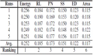
The RCGA is used to find the importance of each features. It defines the weight to each feature according to the objective function defined in eq. (3). As consider crossover rate (CR) and mutation rate (MR) are set to be 0.9 and 0.01
Respectively.Uniform crossover operator is used for crossover and arithmetic mutation (adding or subtracting a small number) is used as mutation operator. After five different runs, the weight obtained for each feature is described in Table 4. We can see in the above table the average weight of energy is highest and area is lowest that also signifies the importance of each feature in the dataset. As the weight given to each feature is significant so all the features are selected for the experiment
where, T is the total number of instances in training data set, R is the RMSD, P is physical and chemical properties, n is the number of properties (6 in this case) and w is the weight given to each feature defined in the range of [0,1].
2.4.2 Machine learning models
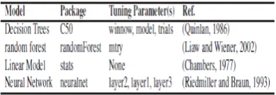
In this work, we used four machine learning models (refer, Table 5) for prediction of RMSD of protein structure. The models are available in R open source software. R is licensed under GNU GPL. In precisely the models is presented below: 1. Decision Trees: This model is an extension of C5.0
classification algorithms described by Quinlan .
2. Random forest: It is based on a forest of trees using random inputs .
3. Linear Models: It uses linear models to carry out regression, single stratum analysis of variance and analysis of covariance .
4. Neural Network: Training of neural networks using back propagation, resilient back-propagation with or without weight or the modified globally convergent version .
3 MODEL EVALUATION
We have many ways to measure performance of the prediction, where some are more suitable than the others depending on the application considered. A brief discussion on the performance measures is explained below. The formula used for all the machine learning models is given by:
Table 5. Machine learning models used
3.1 Root Mean Squared Error
RMSE is a popular formula to measure the error rate of a model. However, it can only be compared between models whose errors are measured in the same units. It is calculated as follows:
Where ,a is actual value, p is predicted value and n is the total number of instances.
3.2 Coefficient of Determination (R2)
The coefficient of determination (R2) summarizes the explanatory power of the model and is computed from the sums-of-squares terms.
3.3 Accuracy
The accuracy is calculated as percentage deviation of predicted RMSD with actual RMSD.
Where , a is actual value, p is predicted value and n is the total number of instances.
3.4 Correlation
Correlation describes the statistical relationships between actual and predicted values. It is defined as follows:
where, x is the actual value, y is the predicted value, ¯x is the mean of the all actual values, ¯y is the mean of the all
predicted values and n is the number of instances. Correlation lies in the range of [0,1] and is considered to be good if its value tends towards 1.
3.5 K-Fold Cross Validation
K-fold cross validation is used to measure accuracy of the predictive model. The original sample is randomly partitioned into k equal size subsamples. Of the k subsamples, a single subsample is retained
as the validation data for testing the model and the remaining k-1 subsamples are used as training data. The cross-validation process is then repeated k times (the folds) with each of the k subsamples
used exactly once as the validation data. Further, the k results from the folds are can be averaged to produce a single estimation. The advantage of this model over repeated random sub-sampling is
that all observations are used for both training and validation, and each observation is used for validation exactly once. Here, 10-fold (k=10) cross validation is used to measure the robustness of the best
selected model. 3.6 Benchmark of local model correctness For the benchmarking of model correctness performance of the random forest model is compared with top-performing ProQ2 (Ray et al., 2012) . Both the benchmark methods are single-model method. ProQ2 is based on Support Vector Machine.
3.6 Benchmark of local model correctness
For the benchmarking of model correctness performance of the random forest model is compared with top-performing ProQ2 (Ray et al., 2012) . The benchmark method is single-model method. ProQ2 is based on Support Vector Machine.
4 RESULTS
In this section, we observe the prediction results of all the four machine learning models on the training and testing dataset. The machine learning models might be suffer from over fitting due to the possibility of criterion used for training the model is not the same as the criterion used to judge the efficacy of a model. Here, to avoid the over fitting , all four machine learning models are run on their default parameters and the distribution of data in training and testing set are 70% and 30% respectively for all the models.
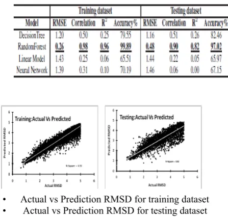
Table 6 shows a comparative performance of all the models in the prediction of RMSD on RMSE, Correlation, R2 and Accuracy. The performance results show that the random forest model outperforms
the machine learning models in the prediction of RMSD of the protein structure in the absence of its true native state. The RMSE is used to measure the differences between values predicted by a model and the values actually observed. The RMSE is calculated using equation 4. The random forest have the lowest
between actual and predicted values and it is calculated using eq. (7). The
random forest have the highest correlation of 0.98 in the training dataset and 0.90 in the testing dataset.
R2 summarizes the explanatory power of the model between the prediction for each observation and the population mean. The R2 is calculated using eq. (5). The random forest have the highest R2 of
Table 6. Performance comparison of all four models on training and testing data set.
• Actual vs Prediction RMSD for training dataset • Actual vs Prediction RMSD for testing dataset
Fig. 4: Scatter plot of Actual vs Predicted values of RMSD on training and testing dataset using random forest
0.96 of in the training dataset and 0.82 in the testing dataset. Fig. 4 shows R2 in training and testing dataset. Accuracy is the degree of consistency of a calculated or measured quantity to its true (actual) value, where as precision is an experiment value, which measures the reliability of an experiment.
The accuracy is calculated using eq. (6) with acceptable error of ±2. The random forest have the highest accuracy of 99.89% in the training dataset and 97.02% in the testing dataset. Here, k-fold (k=10) cross validation is used to measure the robustness of the random forest. Fig. 5 shows the RMSE, correlation, R2 and accuracy for 10 folds in prediction of RMSD .Cross validation results show a uniform performance in all model evaluation parameters. Fig. 4 shows the scatter plot between actual and predicted RMSD for training and testing dataset using random forest. To prove the effectiveness of the predictive model, the performance of random forest is compared with top-performing ProQ2 and the performance is found to be quite impressive (refer, Table 7).
Table 7. Performance validation on the existing decoys sets in the
prediction of RMSD using random forest.
(c) Correlation (d) Accuracy
Fig. 5: 10-fold cross validation of RMSE, R2, Correlation and Accuracy on training and testing data set in the prediction of
RMSD using random forest.
5 CONCLUSION
REFERENCES
[1] Arora, N. and Jayaram, B. (1997). Strength of hydrogen bonds in a helices. Journal of computational chemistry, 18, 1245– 1252.
[2]. Baldi, P. and Pollastri, G. (2002). A machine learning strategy for protein analysis. Intelligent Systems, IEEE, 17(2), 28–35.
[3]. Betancourt, M. R. and Skolnick, J. (2001). Universal similarity measure for comparing protein structures. Biopolymers, 59(5), 305– 309.
[4]. Blanco, A., Delgado, M., and Pegalajar, M. (2001). A real-coded genetic algorithm for training recurrent neural networks. Neural networks, 14(1), 93–105.
[5]. Bryson, K., Cozzetto, D., and Jones, D. (2007). Computer-assisted protein domain Science, 8(2), 181–188.
[6]. Chambers, J. (1977). Computational methods for data analysis. Applied Statistics,(2), 1–10.
[7]. Cheng, J., Sweredoski, M., and Baldi, P. (2005a). Accurate prediction of protein disordered regions by mining protein structure data. Data Mining and Knowledge Discovery, 11(3), 213–222.
[8]. Cheng, J., Saigo, H., and Baldi, P. (2005b). Large-scale prediction of disulphide bridges using kernel methods, two-dimensional recursive neural networks, and weighted graph matching. Proteins: Structure, Function, and Bioinformatics, 62(3), 617–629.
[9]. Durham, E., Dorr, B., Woetzel, N., Staritzbichler, R., and Meiler, J. (2009). Solvent accessible surface area approximations for rapid and accurate protein structure prediction. Journal of molecular modeling, 15(9), 1093–1108.
[10]. Fariselli, P., Olmea, O., Valencia, A., and Casadio, R. (2001). Prediction of contact maps with neural networks and correlated mutations. Protein engineering, 14(11), 835–843.
[11]. Frishman, D. and Argos, P. (1995). Knowledge based protein secondary structure assignment. Proteins, 23(4), 566–579.
[12] Goldberg, D. E. (1990). Real-coded genetic algorithms, virtual alphabets, and blocking Urbana, 51, 61801.
[13]. Herrera, F., Lozano, M., and Verdegay, J. L. (1998). Tackling real-coded genetic algorithms: Operators and tools for behavioral analysis. Artificial intelligencereview, 12(4), 265–319.
[14]. Janin, J. (1979).Surface and inside volumes in globular proteins. [15]. Jones, D. (1999). Protein secondary structure prediction based on
position specific scoring matrices. JMB, 292(2), 195–202.
[16]. Kim, D., Xu, D., Guo, J., Ellrott, K., and Xu, Y. (2003). PROSPECT II: protein structure prediction program for genome-scale applications. Protein engineering,16(9), 641–650.
[17] Krogh, A., Larsson, B., Von Heijne, G., Sonnhammer, E., et al. (2001). Predicting transmembrane protein topology with a hidden Markov model: application to complete genomes. Journal of molecular biology, 305(3), 567–580.
[18]. Liaw, A. and Wiener, M. (2002). Classification and Regression by randomForest. R News, 2(3), 18–22.
[19]. Mittal, A. and Jayaram, B. (2011). Backbones of folded proteins reveal novel invariant amino acid neighborhoods. Journal of Bio molecular Structure and Dynamics, 28
[20]. Narang, P, Bhushan, K., Bose, S., and Jayaram, B. (2006). Protein structure evaluation using and all-atom energy based empirical scoring function. Journal of Bio molecular Structure and Dynamics, 23(4), 385–406.
[21] Obradovic, Z., Peng, K., Vucetic, S., Radivojac, P., and Dunker, A. (2005).Exploiting heterogeneous sequence properties improves prediction of protein disorder. Proteins: Structure, Function, and Bioinformatics, 61(S7), 176–182
[22] Ono, I., Satoh, H., and Kobayashi, S. (1999). A real-coded genetic algorithm for function optimization using the unimodal normal distribution crossover.
[23] PublicDecoy(2010).www.scfbioiitd.res.in/software/pcsm/dataset/Public Decoys. Qiu, J., Sheffler, W., Baker, D., and Noble, W. (2007). Ranking predicted protein structures with support vector regression. Proteins: Structure, Function, and Bioinformatics, 71(3), 1175–1182. [24] Quinlan, J. (1986). Induction of decision trees. Machine learning, 1(1),
81–106.Ray, A., Lindahl, E., and Wallner, B. (2012). Improved model quality assessment using ProQ2. Bioinformatics, 13, 224.
[25] Riedmiller, M. and Braun, H. (1993). A direct adaptive method for faster backpropagation learning: The RPROP algorithm. In Neural Networks, 1993.,IEEE International Conference on, pages 586–591. IEEE. RMSD (2011). http://zhanglab.ccmb.med.umich.edu/TM-score/RMSD.f.
[26] Rost, B. and Sander, C. (1993). Improved prediction of protein secondary structure by use of sequence profiles and neural networks. Proceedings of the National Academy of Sciences, 90(16), 7558– 7562.
[27] Rost, B., Sander, C., et al. (1993). Prediction of protein secondary structure at better than 70% accuracy. Journal of molecular biology, 232(2), 584–599.
[28] Sen, T. Z., Jernigan, R. L., Garnier, J., and Kloczkowski, A. (2005). GOR V server for protein secondary structure prediction. Bioinformatics, 21(11), 2787–2788. Simons, K., Kooperberg, C., [29] Huang, E., Baker, D., et al. (1997). Assembly of protein tertiary
structures from fragments with similar local sequences using simulate annealing and Bayesian scoring functions. Journal of molecular biology, 268(1),209–225.
[30] Travers, A. (1989). DNA conformation and protein binding of b. Annual review biochemistry, 58(1), 427–452.