Construction and Analysis of Word-level Time-aligned
Simultaneous Interpretation Corpus
Takahiro Ono
1, Hitomi Tohyama
2, Shigeki Matsubara
21Graduate School of Information Science, Nagoya University 2Information Technology Center, Nagoya University Furo-cho, Chikusa-ku, Nagoya-shi, 464-8601, Japan
{ono, hitomi, matubara}@el.itc.nagoya-u.ac.jp
Abstract
In this paper, quantitative analyses of the delay in Japanese-to-English (J-E) and English-to-Japanese (E-J) interpretations are described. The Simultaneous Interpretation Database of Nagoya University (SIDB) was used for the analyses. Beginning time and end time of each word were provided to the corpus using HMM-based phoneme segmentation, and the time lag between the corresponding words was calculated as the word-level delay. Word-level delay was calculated for 3,722 pairs and 4,932 pairs of words for J-E and E-J interpretations, respectively. The analyses revealed that J-E interpretation have much larger delay than E-J interpretation and that the difference of word order between Japanese and English affect the degree of delay.
1.
Introduction
Simultaneous interpretation (SI) is one modes of interpreta-tion where the interpreter renders the message in the target language while the source-language speaker continuously speaks, and it is widely used in the international society for its inherent advantages; it has superb time efficiency and rarely disturbs the source-language speaker. Although the SI interpreter and the speaker speak in parallel, the inter-preter’s utterances always delay behind the speaker’s utter-ances to grasp the speaker’s message. Since large delay burdens the interpreter’s memory, which could lower the interpretation quality (Mizuno, 2005), it is essential for in-terpreters to control the delay properly.
The delay is heavily affected by the source and target lan-guages. Because Japanese and English have quite different word order, it is considered that Japanese-to-English (J-E) and English-to-Japanese (E-J) interpretations are difficult. However, few quantitative analyses have been conducted for the interpretations.
In this paper, the quantitative analyses of the delay in J-E and E-J interpretations are discussed. The Simultaneous In-terpretation Database of Nagoya University (SIDB) (Mat-subara et al., 2002) was used for the analyses. We utilized word-level delay to observe the delay inside utterances. To measure the delay efficiently, word-level temporal informa-tion and translainforma-tion correspondences were estimated for the SIDB. The analyses revealed the J-E interpretation’s large delay and other delay characteristics of J-E and E-J inter-pretations.
2.
Corpus
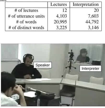
The Simultaneous Interpretation Database of Nagoya Uni-versity (SIDB) (Matsubara et al., 2002) was used in this research. The corpus consists of monologue data (lectures) and dialogue data, and they are accompanied with J-E and E-J interpretations. A part of monologue data was used for the analysis. The statistics of the data used is shown in Ta-ble 1 and 2.
Table 1: Statistics of Japanese lectures and J-E interpreta-tions
Lecture Interpretation
# of lectures 8 13
# of utterance units 3,864 7,461
# of words 24,415 30,026
# of distinct words 2,414 2,976
Table 2: Statistics of English lectures and E-J interpreta-tions
Lectures Interpretation
# of lectures 12 20
# of utterance units 4,103 7,603
# of words 20,995 44,792
# of distinct words 3,225 3,146
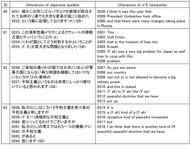
Speaker
Interpreter Speaker
Interpreter
Figure 1: Recording environment of SIDB
1. Estimation of beginning time and end time for all words
2. Extraction of word correspondences
3. Calculation of word-level delay
Step 1 and 2 are explained in detail below.
3.1. Estimation of Word Utterance Timing
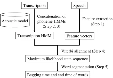
Given speech and its corresponding transcription as input, beginning time and end time of each word are estimated using Hidden Markov Model based phoneme segmentation (Brugnara et al., 1993). The temporal information is esti-mated in the following steps (Figure 4).
1. Feature vectors are extracted from the speech.
Features are 12th order MFCC,∆MFCC, and ∆log energy under the condition shown in Table 3. CMS is done for each utterance unit.
2. Word boundaries and phoneme pronunciation are pro-vided to the transcription.
For Japanese, morphological analyzer ChaSen (Mat-sumoto et al., 1999) is utilized to identify the morpheme boundaries and Katakana pronunciation. Katakana is a Japanese syllabary and it can be con-verted into phoneme sequences by rules. English tran-scriptions are split into words by white spaces and pro-nunciations are given with CMU Pronunciation Dic-tionary version 0.6 (CMU, 1998).
3. Following the pronunciation, phoneme HMMs are concatenated to build the large HMM corresponding to the whole transcript.
For Japanese, the speaker independent 16 mixture monophone model of Julius Dictation Kit v3.1 (Julius, 2005) was used. For English, speaker independent 2 mixture monophone model are constructed from the 6,300 utterances of the TIMIT Acoustic Phonetic Con-tinuous Speech Corpus (Garofolo et al., 1993) using HTK (Young et al., 2006). Three-state left-to-right HMMs are trained for 39 phonemes of CMU Pro-nouncing Dictionary and 1 silence.
4. The maximum likelihood state sequence of the tran-scription HMM is calculated with Viterbi algorithm.
Viterbi algorithm is calculated with speech recogni-tion engine Julius (Julius, 2005).
5. To determine the beginning time and end time for the words, word boundaries are inserted at the time when state transitions between words are occurred.
3.2. Translation Alignment
Given the speaker’s utterances and those of the interpreter, translation correspondences between the speaker’s words and the interpreter’s words are identified. In addition to translation dictionaries, temporal information of words are utilized. Since the interpreter’s word always delay behind the corresponding speaker’s word in SI, only pairs of words which suffice the following conditions are aligned.
Transcription
Transcription HMM
Speech
Feature vectors
Maximum likelihood state sequence Acoustic model
Concatenation of phoneme HMMs
(Step 2, 3)
Feature extraction (Step 1)
Viterbi alignment (Step 4)
Begging time and end time of words
Word segmentation (Step 5)
Figure 4: Overview of word utterance timing estimation
Table 3: Acoustic analysis condition Sampling frequency 16,000Hz
Window function Hamming window
Frame length 25ms
Frame shift 10ms
Pre-emphasis 0.97
Filter bank 24 channels
• Both words are content words.
• The interpreter’s word delays behind the speaker’s one.
• The pair of words are determined to be correspond-ing by dictionary lookup. The dictionary of 100,000 entries was constructed from Eijiro (Eijiro, 2001).
These conditions could find ambiguous correspondences, or many-to-many correspondences. Instead of disambigua-tion, such correspondences are rejected to achieve higher precision.
3.3. Evaluation
The accuracy of the methods explained above was evalu-ated using the SIDB.
To evaluate the estimated temporal information, 10 Japanese utterance units of each were selected for a male speaker, a female speaker, a male interpreter and a fe-male interpreter, and 40 English utterance units were cho-sen in the same manner. The estimated time were compared with manually given annotation, and the accuracy was mea-sured with the average error and the proportion of the word boundaries whose error is less than tolerance values. Table 4 shows the results.
Table 4: Accuracy of word utterance timing estimation
Tolerance value [%]
Language # of word boundaries Average [ms] 20ms 40ms 60ms 80ms 100ms
Japanese 387 28 44.7 77.0 90.2 96.1 98.7
English 308 33 41.9 70.5 86.0 92.9 98.1
0 10 20 30 40 50 60 70 80 90 100
0 1 2 3 4 5 6 7 8 9 10 J-E E-J
[%]
Delay [s]
Figure 5: Delay in J-E and E-J interpretations
4.
Analysis
Quantitative analyses were conducted using the word-level delay. Word-level delay was calculated from 3,722 pairs and 4,932 pairs of words of J-E and E-J interpretations, re-spectively.
4.1. J-E and E-J interpretations
A comparative analysis between J-E and E-J interpretations was conducted. Figure 5 shows the distributions of the de-lay. The width of bins in the cumulative histgrams is 0.2 seconds. The average delay of J-E and E-J interpretations is 4.532 seconds and 2.446 seconds, respectively. The av-erage delay of E-J interpretation is close to other results derived from European language pairs (Barik, 1973) (An-derson, 1994) (Christoffels and de Groot, 2004), while J-E interpretation has larger delay. The difference of verb po-sitions between Japanese and English might have effects. The standard deviation of J-E and E-J interpretations was 4.155 seconds and 2.753 seconds, respectively. The delay of J-E interpretation varies more than E-J interpretation.
4.2. Characteristics of Word
Since Japanese and English have quite different word order, different words might have different delay characteristics. We investigated the correlation of the delay against parts-of-speech (noun or verb) and grammatical roles (subject or object) of the source-speaker’s words.
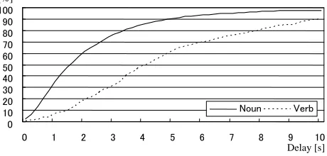
4.2.1. Parts-of-speech
Parts-of-speech were esimated with ChaSen (Matsumoto et al., 1999) and nlparser (Charniak, 2000) for Japanese and English, respectively.
Figure 6 shows the result of J-E interpretation. Although nouns have larger delay than verbs, there is not a large dif-ference. Figure 7 shows the result in E-J interpretation. In E-J interpretation verbs have much larger delay than nouns. There was no significant difference between the distribu-tions of the verbs in Figure 6 and 7. The average delay of verbs in J-E and E-J interpretations was 4.213 seconds
0 10 20 30 40 50 60 70 80 90 100
0 1 2 3 4 5 6 7 8 9 10 Noun Verb
[%]
Delay [s]
0 10 20 30 40 50 60 70 80 90 100
0 1 2 3 4 5 6 7 8 9 10 Noun Verb
[%]
Delay [s]
Figure 6: Delay of nouns and verbs (J-E)
0 10 20 30 40 50 60 70 80 90 100
0 1 2 3 4 5 6 7 8 9 10 Noun Verb
[%]
Delay [s]
Figure 7: Delay of nouns and verbs (E-J)
and 5.073 seconds, respectively, and the difference was about 0.8 seconds. On the other hand, the average delay of nouns in J-E and E-J interpretations was 4.468 seconds and 2.241 seconds, respectively, and nouns of J-E interpre-tation have about twice the delay than E-J interpreinterpre-tation. Grammatical roles of nouns are represented by the position of them in English, while particles are attached to nouns to express their roles in Japanese. The effect of the word order could be reduced by Japanese particles in E-J interpretation, which might result in the smaller delay.
4.2.2. Grammatical Roles
Grammatical roles of Japanese were approximated by at-tached particles. The correlation between the grammatical roles and the delay in J-E interpretation is shown in Table 5. In general, ‘wa’ and ‘ga’ tend to be attached with subjec-tive nouns, and ‘wo’ and ‘ni’ for objecsubjec-tive nouns. Table 5 shows that ‘wa’ and ‘ga’ have smaller delay than ‘wa’ and ‘ni’, that is subjects have smaller delay than objects in J-E interpretation.
Table 5: Attached particles and delay of nouns
Particle to ga wa de ni wo mo no
Frequency 112 265 193 109 211 295 53 354
Average delay [s] 3.964 4.181 4.364 4.733 4.867 4.890 4.930 5.319
0 10 20 30 40 50 60 70 80 90 100
0 1 2 3 4 5 6 7 8 9 10 Noun Numeral
[%]
Delay [s]
Figure 8: Delay of numerals (J-E)
0 10 20 30 40 50 60 70 80 90 100
0 1 2 3 4 5 6 7 8 9 10 Noun Numeral
[%]
Delay [s]
Figure 9: Delay of numerals (E-J)
4.3. Numerals
Section 4.2.1 has shown that nouns have large delay in J-E interpretation. However, since random figures such as date, area, or number of people, are difficult to remember, they might be interpreted with small delay regardless of the source and target languages. The delay of numerals was compared with that of ordinary nouns. Figure 8 shows the result of J-E interpretation. The average delay of numer-als and other nouns were 4.701 seconds and 3.367 seconds, respectively. Figure 9 shows the distributions in E-J inter-pretation, which also shows numerals have smaller delay than ordinary nouns.
5.
Conclusion
Quantitative analyses of the delay in J-E and E-J interpreta-tions have been described. Word-level delay was utilized to observe the delay inside utterances. To measure the delay efficiently, word-level temporal information and translation correspondences were provided to the SIDB automatically. The analyses revealed the following characteristics of the delay:
• J-E interpretation has larger delay than E-J interpreta-tion.
• In J-E interpretation nouns have larger delay than verbs while verbs’ delay is larger than nouns’ one in E-J interpretation.
• In J-E interpretation subjects have smaller delay than objects. No significant difference was found in E-J interpretation.
• Numerals are interpreted quickly regardless of the lan-guage pairs.
6.
References
L. Anderson. 1994. Simultaneous Interpretation: Con-textual and Translation Aspects. In Bridging the Gap: Empirical research in simultaneous interpretation, pages 101–120.
H. C. Barik. 1973. Simultaneous Interpretation: Tem-poral and Quantitative Data. Language and Speech, 18(3):272–287.
F. Brugnara, D. Falavigna, and M. Omologo. 1993. Au-tomatic Segmentation and Labeling of Speech based on Hidden Markov Models. Speech Communication, 12(4):357–370.
E. Charniak. 2000. A Maximum-Entropy-Inspired Parser. In Proceedings of the NAACL-2000, pages 132–139. I. K. Christoffels and A. M. B. de Groot. 2004.
Com-ponents of Simultaneous Interpreting: Comparing Inter-preting with Shadowing and Paraphrasing. Bilingualism: Language and Cognition, 7(3):227–240.
CMU. 1998. CMU Pronunciation Dictionary version 0.6. http://www.speech.cs.cmu.edu/cgi-bin/.
Eijiro. 2001. http://www.eijiro.jp/.
J. S. Garofolo, L. F. Lamel, W. M. Fisher, J. G. Fis-cus D. S. Pallett, and N. L. Dahlgren. 1993. DARPA TIMIT Acoustic-Phonetic Continuous Speech Corpus CD-ROM.
Julius. 2005. http://julius.sourceforge.jp/.
K. Maekawa, H. Koiso, S. Furui, and H. Isahara. 2000. Spontaneous Speech Corpus of Japanese. In Proceed-ings of the LREC-2000, pages 947–952.
S. Matsubara, A. Takagi, N. Kawaguchi, and Y. Inagaki. 2002. Bilingual Spoken Monologue Corpus for Simulta-neous Machine Interpretation Research. In Proceedings of the LREC-2002, pages 167–174.
Y. Matsumoto, A. Kitauchi, T. Yamashita, and Y. Hirano. 1999. Japanese Morphological Analysis System Chasen version 2.0 Manual. In NAIST Techinical Report, NAIST-IS-TR99009.
A. Mizuno. 2005. Process Model for Simultaneous Inter-preting and Working Memory. META, 50(2):739–794. S. Young, G. Evermann, M. Gales, T. Hain, D. Kershaw,