Convolution of large 3D images on GPU and its decomposition

R E S E A R C H

Open Access

Convolution of large 3D images on GPU and its

decomposition

Pavel Karas

and David Svoboda

Abstract

In this article, we propose a method for computing convolution of large 3D images. The convolution is performed in a frequency domain using a convolution theorem. The algorithm is accelerated on a graphic card by means of the CUDA parallel computing model. Convolution is decomposed in a frequency domain using the decimation in frequency algorithm. We pay attention to keeping our approach efficient in terms of both time and memory consumption and also in terms of memory transfers between CPU and GPU which have a significant inuence on overall computational time. We also study the implementation on multiple GPUs and compare the results between the multi-GPU and multi-CPU implementations.

Keywords:convolution, decomposition, Fourier transform, FFT, GPU, CUDA

1 Introduction

The convolution of two signals can be employed for blurring images, deconvolving blurred images, edge detection, noise suppression, and in many other applica-tions [1-3]. For example, a cross-correlation and a phase-correlation (which are important methods of image registration) are both very similar to a convolu-tion since they have basically the same mathematical meaning except that a convolution involves reversing a signal [[1], p.211]. The convolution of large signals is also used for simulating image formation in optical sys-tems such as light microscopes [4]. The convolution is a common method used in image processing; however, its computation is very time-consuming for large images. Graphic cards can be employed for accelerating the computation. Some of the algorithms can be found in NVIDIA whitepaper [5]. Here, a so-called naïve convo-lution and a convoconvo-lution with separable kernel are described, along with their optimized GPU implementa-tion in CUDA. These algorithms can be used in many applications, such as fast computation of Canny edge detection [6,7]. However, these approaches are not suita-ble for general large kernels.

In optical microscopy, we often deal with both large input signals and kernels. Thus, in this article, we

discuss the time complexity of a convolution with emphasis on large 3D images. We recall the convolution theorem and its positive effect on the time complexity. For example, having a signal of 1000 × 1000 × 100 vox-els and a filter kernel of 100 × 100 × 100 voxvox-els, which is common in optical microscopy, the calculation using the convolution theorem takes tens of seconds, instead of several days, on the most recent CPU architecture. Even better times can be obtained using graphic cards. The GPU-based convolution using the convolution the-orem is described in [8]. As indicated by authors, the FFT-based approach is suitable for large non-separable kernels.

The essential part of the algorithm described above is the Fourier transform. The first attempt to compute the fast Fourier transform on graphics hardware was described in [9]. The implementation was written in OpenGL and Cg shading languages and tested in the convolution application. The comparison of convolution in spatial and frequency domain (for the description of both approaches refer to the following section) was made in [10]. A significant speedup was achieved by implementing the algorithm on GPU, using HLSL and DirectX. Recently, the NVidia® CUDA programming model [11] along with the CUFFT library [12] offers a framework for implementing convolution in a straight-forward manner. Besides CUFFT, other FFT libraries for GPU were developed, such as [13] and [14]. The * Correspondence: [email protected]

Centre for Biomedical Image Analysis, Faculty of Informatics, Masaryk University, Botanicka 68a, Brno, Czech republic

OpenCL framework allows implementing methods on heteregenous platforms, consisting of CPU, GPU and other architectures [15,16].

The bottleneck of the GPU acceleration is that gra-phics hardware offers rather small amount of memory. This poses a significant problem to attempts of acceler-ating convolution of huge images on GPU. Due to con-volution properties, the convolved image can be divided into arbitrarily small parts, but all the sub-images have to be extended with neighboring pixels of at least size of the filter kernel (point spread function–PSF), as described in [17]. Thus, a lot of redundant computation needs to be performed, proportionally to the PSF size. This approach was successfully used in [18], to compute spatially variant deconvolution of Hubble Space Tele-scope images. We propose a new approach, which is optimal, in terms of both the number of per-voxel com-putations and the number of memory transfers.

1.1 Convolution

A 1D convolution of two discrete finite signals f, g is defined by following [19]:

[f∗g](n)≡

Mg−1

m=0

f(n−m)g(m), n= 0,. . .,M−1,(1)

whereMfand Mgis the number of samples offandg,

respectively. The convolution then produces a signal of sizeM =Mf+Mg- 1. For the list of conventions used in

the article refer to Appendix A.

Obviously, we have to take into account the boundary conditions defining f(m) at m < 0 and m >Mf - 1

[19,20]. Usually we set

f(m)≡0, (m<0)∨(m>Mf−1) (2a)

(Dirichlet boundary conditions) or

f(m)≡

f(0), m<0,

f(Mf−1),m>Mf −1 (2b)

(Neumann boundary conditions).

In practice, one of the signals has usually significantly larger size and is called simply thesignal whereas the other is of a smaller size and is called thefilter kernel. For instance, a kernel can be given by a simple function, such as Gaussian, or by so-called PSF, a function that describes the impulse response of an imaging system to a point source [[3], pp. 205-207].

A computation of convolution can be very time-con-suming. From Equation (1) it can be easily deduced that the time complexity of the problem isO(MfMg). In the

case the kernel is small (tens of samples) the convolu-tion can be computed in a reasonable time, even for large signals. However, in some applications such as

optical microscopy one deals with both signals and ker-nels of more than a million of samples each. In this case computation would take several days which is unaccep-table and a different solution needs to be applied.

1.2 Convolution theorem

The convolution theorem provides us with a powerful tool for convolving large signals. Having two signals f, g

it can be proved that

Ff ∗g=FfFg, (3a)

f∗g=F−1(F[f]F[g]), (3b)

where F denotes a Fourier transform. Therefore, instead of a convolution according to the definition, Fourier transforms can be applied on both the signal and the kernel, then their pointwise product is com-puted and finally inverse Fourier transform is applied to obtain the result [19].

Keep in mind that before the computation both the sig-nal and the kernel need to be padded to the same size (that is, to the size of the resulting convolved signal) to avoid problems with boundary values. For example, in 1D case both the signal and the kernel are padded toM=Mf

+Mg- 1 samples. There are several ways how to pad the

data, usually they are padded with zeros. The position of the padding influences the position of the resulting signal. Refer to [19] for more details. According to the convolu-tion theorem the asymptotic time complexity of a convo-lution is the complexity of FFT [19,21], i.e.,O(MlogM).a

1.3 Memory complexity

As we mentioned in the previous section, to be able to apply the convolution theorem both the signal and the kernel have to be padded before computation. Hence, aM bytes of memory is required to store signal and the same amount for kernel, thus 2aMbytes in total where ais the size of data type used, e.g., typically 4 bytes for a single precision.

The Fourier transform can be performed in-place on a complex signal, so no additional memory is required. If the Fourier transform is performed on a real signal, the following property holds:

F(μ) =F∗(M−μ), μ= 0,

F(0) =F∗(0), (4)

2 Method

2.1 GPU accelerated convolution

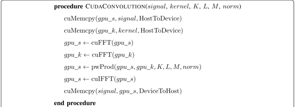
In this section, we describe a basic GPU-based imple-mentation of convolution using CUDA. CUDA is a par-allel computing model introduced by the nVidia company. It provides C language extensions to imple-ment pieces of code on GPU. This so-called CUDA Toolkit also includes the CUBLAS and the CUFFT libraries providing algorithms for linear algebra and fast Fourier transform, respectively.

Using the Toolkit, an implementation of a convolution is quite simple and straightforward, see the example in Figure 1. Basically, the algorithm consists of three parts: First, the data are transferred from CPU (host) memory to GPU (device) memory. Then, the Fourier transform, the pointwise multiplication, and the inverse Fourier transform are subsequently performed. Finally, the data are transferred back to the host memory.

The pointwise multiplication is done in a simple loop so its parallelization is straightforward. GPU threads are mapped to individual image pixels, natu-rally providing coalesced memory accesses and mas-sive parallelism. This approach is thus simple and optimal, limited by a global memory bandwidth only. For basic information and examples refer to the CUDA Programming Guide document and CUDA SDK samples [11,23].

The Fourier transform parallel computations are pro-vided by the CUFFT library [12], as it is presently to our best knowledge the best library for FFT computa-tion on GPU. In this part of the algorithm, all the opti-mizing issues (e.g., memory coalescing, shared or texture memory usage, etc.) are concerns of the CUFFT library.

When dealing with both large 3D images and large kernels it is impossible to compute convolution at once on GPU since the recent graphic cards typically have about 1GB of memory. This is also due to CUFFT speci-fics–if an image is too large to be stored in a shared memory, the FFT is performed out-of-place. As a result, even more memory is required [12]. In this section, we propose an algorithm for the decomposition of convolu-tion. First, we describe the decimation in frequency (DIF) algorithm. This approach is not new, it was used, e.g., in [10], to provide the whole FFT computation. However, our contribution is to employ the DIF method to decompose data, i.e., to prepare it for convolution so that it can be processed in parts.

It should be noted that there are several other approaches to decompose the FFT problem, however, they are sub-optimal in means of the number of per-pixel operations and data transfers. First, the DIT method can be used instead of the DIF. However, unlike the DIF, this approach does not provide complete separ-ability of the resulting sub-problems. This leads to a lot of redundant data transfers. Second, in the spatial domain, the convolved image can be divided into small parts. This method will be referred to as the tiling. However, all the sub-images have to be extended with neighboring pixels of at least size of the filter kernel [17]. Thus, a lot of redundant computation needs to be performed, proportionally to the PSF size.

The comparison of three approaches to divide the convolution problem is shown in Table 1. Mfand Mg

denote the size of the signal and kernel, respectively,cis a constant corresponding to a per-pixel number of arithmetic operations needed for the computation of FFT, andP denotes the number of parts the input data

procedure

C

C

(

signal

,

kernel

,

K

,

L

,

M

,

norm

)

cuMemcpy(

gpu s, signal,

HostToDevice)

cuMemcpy(

gpu k, kernel,

HostToDevice)

gpu s

←

cuFFT(

gpu s

)

gpu k

←

cuFFT(

gpu k

)

gpu s

←

pwProd(

gpu s, gpu k, K, L, M, norm

)

gpu s

←

cuIFFT(

gpu s

)

cuMemcpy(

signal, gpu s,

DeviceToHost)

end procedure

are divided into. The DIF method is the only one which is not depend on thePparameter.

2.2 Decimation in frequency

The DIF algorithm is a technique used in fast Fourier transform to split data into several disjoint parts. We will introduce the idea for 1D case first. Let us have a functionf(m) and its Fourier transformF(μ), m, μ= 0, ...,M - 1. Supposing that M is even we introduce new functionsr(m’) ands(m’), m’= 0, ...,M/2 - 1 as follows [22,24]:

r(m)≡f(m) +f(m+M/2), (5a)

s(m)≡[f(m)−f(m+M2)]W_M−m, (5b)

where_W M=ei

2π

M is a base function of a Fourier trans-form. Vice versa, it is simple to deduce

f(m) = 1 2

r(m) +s(m)W_Mm, (6a)

f(m+M2) = 1 2

r(m)−s(m)W_Mm. (6b)

Then it can be proved that the Fourier transformsR

(μ’) andS(μ’) of the functions fulfil the following prop-erty:

R(μ) =F(2μ), (7a)

S(μ) =F(2μ+ 1). (7b)

As explained above, the input function f can be decomposed into two half-sized partsr ands. The most important property ofrandsis that they are completely separated parts of the original function in the frequency domain. Furthermore, the DIF algorithm can be applied recursively on the functions r and s, so the functionf

can be decomposed into four parts, then into eight parts, etc., supposing thatM is divisible by 4, 8, .... Fig-ure 2 depicts a scheme of the DIF algorithm.

The decomposition can be employed in n-D case. Since a Fourier transform is separable, ann-D transform can be expressed as a sequence of 1D transforms. Hence, the decomposition can be applied in any dimen-sion. For 3D signals, a decomposition inzdimension–or the first coordinate in a row-major order–should be applied so that P separated parts in P continuous blocks of a memory are obtained. Unlike interlaced data, continuous blocks are optimal for data transfers.

2.3 Implementation

In this section, we introduce a modified algorithm for computing a convolution of large 3D images on GPU. The algorithm uses the DIF method for decomposing data. If the data are complex then the decomposition

Table 1 Methods for decomposition of the convolution problem and their requirements

Method Number of operations Number of memory transactions

DIF c(Mf+Mg) log(Mf+Mg) + (Mf+Mg) 3(Mf+Mg)

DIT c(Mf+Mg) log(Mf+Mg) + 2(Mf+Mg) (2 +P)(Mf+Mg)

Tilling _c(Mf+P_{Mg) log(}Mf

P +Mg) + (Mf+ 2PMg) 2Mf +(P+ 1)Mg

Figure 2Buttery scheme of the DIF. Equation (5) is applied on the signalfof length 8 (the black points) and then two discrete Fourier transform of the half size are performed. The transformed signalFis the result.

can be performed in-place, whereas if the data are real then the decomposition need to be performed out-of-place. The real data could also be transformed into a complex form but it is rather ineficient.

For the out-of-place decomposition of the data, 2aKLMbytes are required for storing the signal and the kernel and 4aKLMbytes for the decomposed data since complex numbers use up twice the size of real numbers. Thus, the overall memory space required is 6aKLM

bytes.

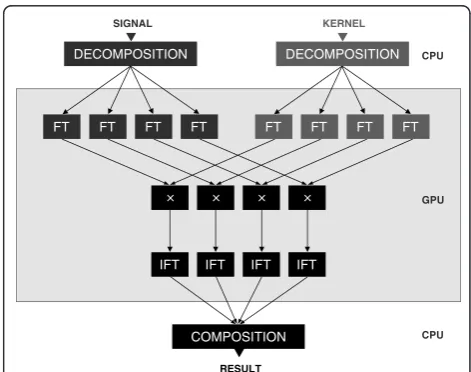
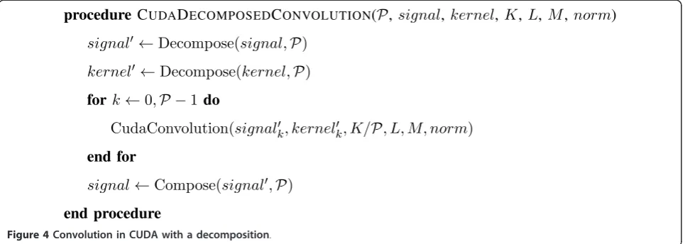
A general review of the algorithm is shown in Figure 3, full description is in Figure 4. It is assumed that size of the data inz dimension is divisible by P, otherwise the data need to be padded to the nearest multiple ofP before the convolution. However, it does not introduce a significant overhead to the algorithm since the size of the padding, if needed, is less than 1% of the overall image size.

Our implementation offers (de)compositions into 2, 4, 8, or 16 parts. These are provided by particular proce-dures named Decompose2, Decompose4, Decompose8, and Decompose16 (and analogously Compose2, etc.). The Decompose2 and Compose2 procedures conduct Equations (5) and (6), respectively. The Decompose4 and Compose4 may either recursively call the Decom-pose2 and ComDecom-pose2, respectively, or they may directly split the data into four parts and reconstruct back from the four parts, respectively. We have opted for the latter solution since it requires smaller number of operations per voxel. Refer to Appendix B for more details.

The remaining procedures were implemented as fol-lows:

Decompose8 = Decompose4 ◦ Decompose2, Decompose16 = Decompose4 ◦ Decompose4,

Compose8 = Compose2 ◦ Compose4, Compose16 = Compose4 ◦ Compose4,

where∘denotes a composition of operations.

2.4 Multi-GPU implementation

Since the decomposition separates the convolution into

P parts it is plain enough to solve the problem by mul-tiple GPUs. To analyze precisely the contribution of the multi-GPU implementation we have to examine times spent in individual phases of the algorithm. In the sin-gle-GPU implementation described in Section 2.3 the overall timeTcan be expressed as follows:

T= max(tp+td,ta) +th→d+tconv+td→h+tc, (8)

where tpis the time required for the padding of the

data,tdfor decomposition,tafor allocating memory and

setting up FFT plans on GPU,th®d for data transfers

from CPU to GPU (host to device), tconv for the

convo-lution itself,td®hfor data transfers from GPU to CPU

(device to host) and finally tc for composition. Despite

the fact that most time is spent in the convolution phase, the other phases cannot be neglected. Please note that the ta time needed for preparing the GPU can be

overlapped with the tpandtdtimes needed for

prepar-ing the data on CPU.

Supposing thatGGPUs are available and, for the sake of simplicity,P is divisible byG, the overall timeT’can be expressed as follows:

T= maxtp+td,ta +th→d+

tconv

G +td→h+tc, (9) assuming that data cannot be transferred to multiple devices concurrently so both the times th®dand td®h

remain the same. As a result, a data transfer of two image tiles from CPU to two GPUs concurrently–that is one tile to each GPU–lasts double the time of a data transfer of one tile to a single GPU. Actually, the overall time complexity of multi-GPU implementation can be even better than determined in Equation (9) because the

procedure

C

D

C

(

P

,

signal

,

kernel

,

K

,

L

,

M

,

norm

)

signal

←

Decompose(

signal,

P

)

kernel

←

Decompose(

kernel,

P

)

for

k

←

0

,

P −

1

do

CudaConvolution(

signal

, kernel

, K/

P

, L, M, norm

)

end for

signal

←

Compose(

signal

,

P

)

end procedure

data transfers can be overlapped by computations on those GPUs that already possess the data (see Figure 5). The precise time values differ in particular situations. In general, they depend on the ratio of the data transfers and the convolution itself so Equation (9) can be consid-ered as the upper estimate.

The final multi-GPU implementation is described in algorithm in Figure 6. Also a simple implementation of a custom cuMemcpy function is described in Figure 7. This function guarantees unique memory access enabling faster overall computation time in this way.

3 Results

We have performed several benchmarks on a machine with the Intel® Core™ i7 950 processor with 6 GB DDR3 RAM and the nVidia® GeForce GTX 295 gra-phic card with 2 × 896 MB GDDR3 RAM. The CPU implementation uses the FFTW library while the GPU implementation uses our algorithm. Both the decom-position and the comdecom-position are performed on CPU. Therefore, we have written them in C language and further improved with SSE intrinsics for a better performance.

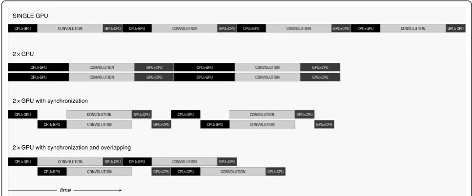
Figure 5Timeline: single-GPU versus multi-GPU (a model situation). The dark boxes depict data transfers between CPU and GPU while the light boxes represent convolution computations. In the first row there is the single-GPU implementation. In the second row there is a timeline for parallel usage of two GPUs. The data transfers are performed concurrently but through a common bus, therefore they last twice longer. For the third row the data transfers are synchronized so that only one transfer is made at a time. In the last row the data transfers are overlapped with a convolution execution.

procedure

C

M

G

C

(

P

,

G

,

signal

,

kernel

,

K

,

L

,

M

,

norm

)

signal

←

Decompose(

signal,

P

)

kernel

←

Decompose(

kernel,

P

)

for

l

←

0

,

G −

1

do

Parallel loop

selectDevice(

l

)

CudaDecomposedConvolution(

P

/

G

, signal

, kernel

, K/

G

, L, M, norm

)

end for

signal

←

Compose(

signal

,

P

)

end procedure

3.1 Single GPU implementation

The single GPU implementation was compared with a single thread CPU implementation. Considering the CPU implementation two approaches are distinguished: The one using both complex-to-complex FFT and inverse FFT (we call it the c2c implementation) and the one using real-to-complex FFT and complex-to-real inverse FFT (the r2c implementation). The former implementation can generally be used for convolving complex data (much like our approach), the latter one can be used on real data only but is twice as effective (in means of both the memory requirements and the speed).

In the first dataset (Table 2) the images are padded to the powers of two in each dimension so we refer to them as tospecifically sizedimages. This property has a significant inuence on computation time because on these images the FFT algorithm performs the best. In the second dataset (Table 3) the images arearbitrarily sized except that in thez dimension the padded size is

kept so that the decomposition can be performed with-out the need of additional image padding.

In all tests, the decomposition parameterP was set to the least possible value so that the resulting sub-images fitted into GPU memory. For example, if the image was small enough, the decomposition was not performed at all, the larger the image was the more parts it was decomposed into.

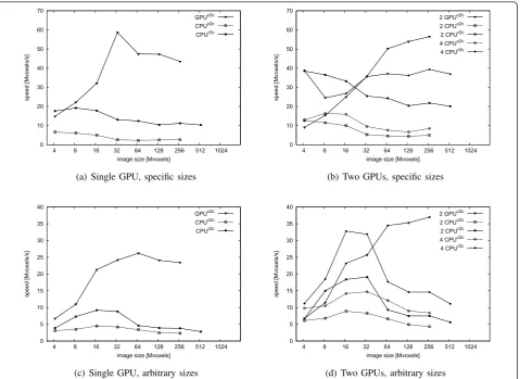
The computation times are presented in Tables 2 and 3. For the sake of understandability the times were also converted into computation speed (number of voxels processed per second), see Figure 8(a),(c).

The results show that a single-GPU implementation is more than ten times faster as compared to a single thread CPU c2c implementation and about four times faster than a single thread CPU r2c implementation if the images are large enough. The r2c approach is the only one which can process images with sizes of more than 500 megavoxels. This is due to the limitations of the CPU memory.

We can also see that in the case of specifically sized images the difference between the time values is small for images smaller than 10 megavoxels. Nevertheless, in practise the arbitrarily sized images are more frequent. In this case, the GPU implementation is faster even on smaller images.

3.2 Multi-GPU implementation

In the second experiment, the multi-GPU implementa-tion (using both the GPUs of GTX 295) was compared with a multiple thread CPU implementation. The same dataset was used, e.g., both the specifically sized and the arbitrarily sized images. The results are presented in Tables 4 and 5 and in Figure 8(b),(d).

The results reveal several facts. Again, the GPU imple-mentation is up to eight times faster than the CPU c2c implementation (depending on image sizes) and up to three times faster than the CPU r2c implementation when comparing two GPUs with two CPU cores. Also a test with four CPU cores was made and the GPU imple-mentation has performed still two times faster if the

Table 2 Convolution of specifically sized images

Image size Time (s)

Image x×y×z [Mpx] P GPUc2c _CPUr2c _CPUr2c

1 256 × 256 × 64 4.2 1 0.3 0.6 0.2

2 512 × 256 × 64 8.4 1 0.4 1.4 0.4

3 512 × 512 × 64 16.8 1 0.5 3.4 0.9 4 512 × 512 × 128 33.6 2 0.6 13.2 2.6 5 1024 × 512 × 128 67.1 4 1.4 29.3 5.4 6 1024 × 1024 × 128 134.2 8 2.8 54.3 12.9 7 1024 × 1024 × 256 268.4 16 6.2 104.3 24.0 8 2048 × 1024 × 256 536.9 – – – 52.2

Table 3 Convolution of arbitrarily sized images

Image size Time (s)

Image x×y×z [Mpx] P GPUc2c CPUc2c CPUr2c

9 257 × 257 × 64 4.2 1 0.6 1.4 1.1

10 513 × 257 × 64 8.4 1 0.8 2.4 1.2 11 513 × 513 × 64 16.8 1 0.8 3.7 1.8 12 513 × 513 × 128 33.7 2 1.4 8.0 3.8 13 1025 × 513 × 128 67.3 4 2.6 19.8 14.7 14 1025 × 1025 × 128 134.5 8 5.6 52.8 34.8 15 1025 × 1025 × 256 269.0 16 11.5 118.9 70.5 16 2049 × 1025 × 256 537.7 - - - 189.0

procedure CULOCKEDMEMCPY(to,f rom,direction)

whilelock do

Wait()

end while

lock←_true

cuMemcpy(to, f rom,_direction)

lock←_false

end procedure

images were large enough. In general, the GPU imple-mentation becomes advantageous on images larger than 50 megavoxels.

Note that in some cases a single GPU has performed better than two GPUs (especially in the case of specifi-cally sized images). We shall see in the following section that the algorithm spent too much time in preliminary

phases (such as data decomposing or memory allocat-ing) at the expense of the convolution itself.

3.3 Time analysis

We have analyzed the time distribution of the phases of the proposed algorithm on two images with a resulting image size of 640 × 640 × 128 voxels. Our method was tested with different settings of the parameter P

0 10 20 30 40 50 60 70

4 8 16 32 64 128 256 512 1024

speed [Mvoxels/s]

image size [Mvoxels]

GPUc2c CPUc2c CPUr2c

(a) Single GPU, specific sizes

0 10 20 30 40 50 60 70

4 8 16 32 64 128 256 512 1024

speed [Mvoxels/s]

image size [Mvoxels]

2 GPUc2c 2 CPUc2c 2 CPUr2c 4 CPUc2c

4 CPUr2c

(b) Two GPUs, specific sizes

0 5 10 15 20 25 30 35 40

4 8 16 32 64 128 256 512 1024

speed [Mvoxels/s]

image size [Mvoxels]

GPUc2c CPUc2c CPUr2c

(c) Single GPU, arbitrary sizes

0 5 10 15 20 25 30 35 40

4 8 16 32 64 128 256 512 1024

speed [Mvoxels/s]

image size [Mvoxels]

2 GPUc2c 2 CPUc2c 2 CPUr2c 4 CPUc2c 4 CPUr2c

(d) Two GPUs, arbitrary sizes

Figure 8The computation speed (in Megavoxels per second) on different datasets (specifically and arbitrarily sized) and configurations (single and multiple GPUs). Comparison between CPU and GPU.

Table 4 Multi-GPU convolution of specifically sized images

Time (s)

Image 2GPUc2c 2CPUc2c 2CPUr2c 4CPUc2c 4CPUr2c

1 0.5 0.3 0.1 0.3 0.1

2 0.5 0.7 0.2 0.5 0.3

3 0.7 1.7 0.5 1.1 0.6

4 0.9 6.3 1.3 3.5 0.9

5 1.3 14.5 2.8 8.9 1.8

6 2.5 30.7 6.6 19.9 3.7

7 4.8 53.4 12.3 31.4 6.8

8 - - 26.7 - 14.5

Table 5 Multi-GPU convolution of arbitrarily sized images

Time (s)

Image 2GPUc2c 2CPUc2c 2CPUr2c 4CPUc2c 4CPUr2c

9 0.6 0.7 0.6 0.4 0.4

10 0.7 1.2 0.6 0.8 0.5

11 0.7 1.9 0.9 1.2 0.5

12 1.3 4.1 1.8 2.3 1.1

13 2.0 10.2 7.2 5.6 3.8

14 3.8 27.6 17.9 14.9 9.2

15 7.3 62.0 36.0 32.0 18.4

(number of decomposed parts). The results are depicted in Figure 9(a).

The convolution itself consumes slightly less than a half of the overall time. The rest is spent on the other phases such as the preparation phase (memory alloca-tion and setting up FFT plans [12] on GPU; and the data padding and the data decomposition on CPU), data transfers between CPU and GPU and finally the data composition. As the preparation phases on GPU on CPU are independent, they can be conducted simulta-neously. The results can be confronted with Equation 8. Here, the “Pad”,“Decompose”,“Allocate”,“CPU>GPU”,

“Convolution”,“GPU>CPU”, and“Compose”times cor-respond totp,td,ta,th®d, tconv,td®h, and tc, respectively.

In the case of the multi-GPU implementation the time spent in the preparation phase on GPU tais double, see

Figure 9(b). This unpleasant behavior is also observed on a machine with CUDA 4.0 with extended support for multi-GPU processing [25]. To the best of our knowl-edge, it is not mentioned in official NVIDIA documents. Fortunately, the time needed for padding the data on

CPUtpis still larger. Thus, the overhead inducted byta

is hidden by tp. The times confronted with Equation 9

give us a good idea of how the usage of multiple GPU cards can speed up the computation. Since the signifi-cant portion of time is spent in sequential phases of the algorithm, the overall speedup is limited, corresponding to the famous Amdahl’s law [26].

We may draw the conclusion that it is reasonable to choose the smallest value possible forP for given image size. The exact results depend on particular dataset. Sometimes, one may prefer usage of the (De)Compose4 function instead of the (De)Compose2 function–and therefore settingP to 4 instead of 2, or to 16 instead of 8–since these two functions are equally efficient and the Fourier transforms may be more efficient on the smaller parts of the decomposed image, rather than on the lar-ger parts.

3.4 Precision analysis

We tested our algorithm for real data from optical microscopy. The bit depth of the images was 16 bits;

0 400 800 1200 1600 2000 2400

2 4 8 16

time [ms]

P

CPU: Compose

Idle time Decompose Pad

CPU:

GPU: GPU>CPU Convolution CPU>GPU Idle time Allocate

(a) Single GPU

0 400 800 1200 1600 2000 2400

2 4 8 16

time [ms]

P

CPU: Compose

Idle time Decompose Pad CPU:

GPU 1+2: GPU>CPU Convolution CPU>GPU Idle time Allocate

(b) Two GPUs

Figure 9Time analysis of the proposed convolution algorithm. The charts describe time (y-axis) spent in particular phases of the proposed algorithm depending on decomposition parameterP(x-axis). In the single-GPU implementation there are two parallel timelines, one for CPU, one for GPU. In the multi-GPU implementation two GPUs have been tested. Thus, there are three parallel timelines, one for CPU and one for each GPU. The overall time of the algorithm is equal to the top of the CPU timeline.

Table 6 Precision analysis of specifically sized images

Image size δ[10-3] (single) δ[10-3] (double)

Image x×y×z [Mpx] P=1 P=2 P=4 P=8 P=16 P=1,. . .,16

1 256 × 256 × 64 4.2 0.12 0.11 0.12 0.11 0.12 0.004

2 512 × 256 × 64 8.4 0.16 0.15 0.15 0.14 0.14 0.006

3 512 × 512 × 64 16.8 0.18 0.17 0.20 0.18 0.20 0.007

4 512 × 512 × 128 33.6 - 0.22 0.22 0.24 0.23 0.015

5 1024 × 512 × 128 67.1 - - 0.26 0.25 0.25 0.019

6 1024 × 1024 × 128 134.2 - - - 0.28 0.29 0.018

7 1024 × 1024 × 256 268.4 - - - - 0.26

-however, the actual bit depth of the image contents was approximately 10-11 bits. This is often the case in the optical microscopy since the bit depth is limited by both parameters of CCD sensors, such as the accuracy of the A/D convertor, and the imaging conditions, namely the amount of light. The convolution normalized with the sum of the kernel values was computed and the results of the CPU implementation and the GPU implementa-tion, both in single precision, were compared. Then the maximum difference between the two resulting images over all voxels was computed:

δ= max{|Ci−Gi|,i∈}, (10)

where Ci is the voxel value at the position i in the

image computed by CPU, Gi is the voxel value at the

positioni in the image computed by GPU andΩis the set of all coordinates in the image.

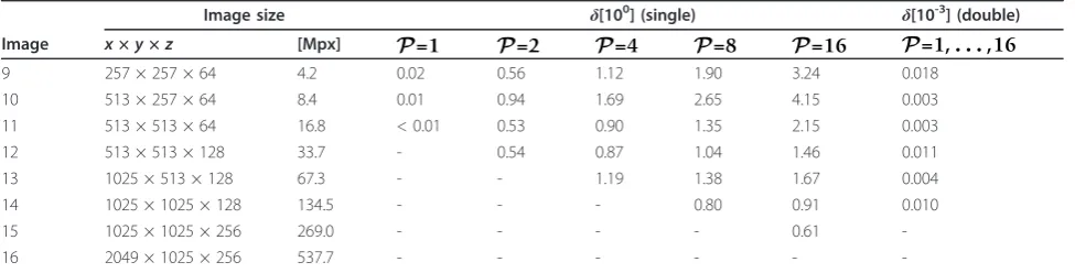
The results for different settings of the parameterP as for both single and double precision are shown in Tables 6 and 7. For the latter, the results were approxi-mately the same for all values of P, therefore only one column is shown for the sake of simplicity. As expected, the precision is not an issue for specifically sized images. For single precision the error is lower than 10-3, for double it is even lower or equal to 10-5. However, it starts to become an issue for arbitrarily sized images. As results show, the error rate depends not only on the overall image size, but also on the individual dimen-sions. In particular, the error is significantly higher for images of dimensions that cannot be factored into small primes. Thus, the worst results (δ > 1) were achieved for image where one dimension was equal to 257, which is prime itself. In some cases, image padding can be used to achieve better accuracy. For those applications where the accuracy is essential, the double precision is still required.

We find that for images of sizes that can be factored into small primes single precision is acceptable for most purposes. However, we are aware that in some applica-tions single precision might not be enough. The recent nVidia graphic cards offer computing in double

precision, however the speed is too low (1/8 of the speed in single precision). With the release of the Fermi architecture computing in double precision on GPU will become feasible.

4 Conclusion

In this article, we have proposed a new method for con-volving large images. We have taken advantage of high computation power of GPU and extended the algorithm with a decomposition. As a result we are able not only to convolve images larger than the size of GPU memory, but also to employ multiple GPUs in parallel.

Our method is generally suitable for complex data. However, in the case of real data it is rather inefficient. Since the input data are represented by the complex numbers with zero imaginary parts, and not by the real numbers, double effort is made to compute the result. On the other hand, the method can be optimized for real data in a few ways [22,24,27]. This is the subject of our future study.

The results show that it is reasonable to use our algo-rithm especially on very large images where the speedup of the GPU implementation can be up to 5× for the complex data and 2-3× for the real data. We suggest to decompose images into the smallest number of parts possible as this approach seems to be the most efficient.

We also studied the precision of the convolution in a practical application. The results revealed that for this application the computation in a single precision is acceptable (and it will be probably so for many other applications). In the case the single precision is not enough it is also possible to compute in a double preci-sion. However, in this precision the recent graphic cards perform poorly. With the release of new architectures (e.g., nVidia Fermi) double precision will become feasible.

The proposed method can be implemented also in OpenCL and other languages besides CUDA. Besides the graphic cards, other parallel architectures can be taken into account as well. As the convolution is a key part of many deconvolution methods [28,29], application

Table 7 Precision analysis of arbitrarily sized images

Image size δ[100] (single) δ[10-3] (double)

Image x×y×z [Mpx] P=1 P₌₂ P=4 P₌₈ P=16 P=1,. . .,16

9 257 × 257 × 64 4.2 0.02 0.56 1.12 1.90 3.24 0.018

10 513 × 257 × 64 8.4 0.01 0.94 1.69 2.65 4.15 0.003

11 513 × 513 × 64 16.8 < 0.01 0.53 0.90 1.35 2.15 0.003

12 513 × 513 × 128 33.7 - 0.54 0.87 1.04 1.46 0.011

13 1025 × 513 × 128 67.3 - - 1.19 1.38 1.67 0.004

14 1025 × 1025 × 128 134.5 - - - 0.80 0.91 0.010

15 1025 × 1025 × 256 269.0 - - - - 0.61

-of the proposed algorithm in the deconvolution will also be the subject of our future study.

Endnotes

a

In 3D case both signals are padded to size M =Mf+

Mg- 1 in xdimension, L=Lf+Lg- 1 in ydimension

and K=Kf +Kg- 1 in z dimension; and the resulting

complexity is O(KLMlog(KLM)). bSupposing the data are stored in a memory in a row-major order, the last dimension is thexdimension.

Acknowledgements

This work was supported by the Ministry of Education of the Czech Republic (Projects No. MSM-0021622419, No. LC535, and No. 2B06052).

Appendix .1 Conventions

We introduce the conventions used in the text:

•f*g... convolution of signalsf,g •Ff... Fourier transform of a signalf

•_F−1_{[F]... inverse Fourier transform of a signalF}

•f(m) ... a signal is denoted by a lowercase letter with a Latin letter index •F(_μ) ... a Fourier transform is denoted by an uppercase letter with a greek letter index

•_W

M= ei

2π

M . . .a base function of a Fourier transform

In 1D case we introduce

•Mf,Mg... sizes of the signal and the kernel, respectively •M=Mf+Mg- 1 ... size of the output convolved signal In 3D case we introduce

•Kf,Lf,Mf... sizes of the signal in dimensionsz,y,x, respectively •Kg,Lg,Mg... sizes of the kernel in dimensionsz,y,x, respectively •K,L,M... sizes of the output convolved signal in dimensionsz,y,x, respectively (K=Kf+Kg-1, etc.)

.2 Decimation in frequency

A signalf(m)can directly be decomposed into four parts by applying Equation 5 recursively:

r(m)

t(n) ≡r(n) +r(n+M/4),

u(n)≡[r(n)−r(n+M/4)]W_M−n_/2; (11a)

s(m)

v(n) ≡s(n) +s(n+M/4),

w(n)≡[s(n)−s(n+M/4)]W_M−n_/2, (11b)

wheren= 0, ...,M/4 - 1. Then the Fourier transformsT(ν),U(ν),V(ν), andW (ν) hold the following property:

T(v) =F(4ν), (12a)

U(v) =F(4ν+ 2), (12b)

V(v) =F(4ν+ 1), (12c)

W(v) =F(4ν+ 3). (12d)

Now let us introduce

o≡n+M/4, p≡n+M/2, q≡n+ 3M/4,

then it can be proved that

t(n) =x(n) +x(o) +x(p) +x(q), (13a)

u(n) = (x(n)−x(o) +x(p)−x(q))W_M−2n, (13b)

v(n) = [(x(n)−x(o))−i(x(p)−x(q))]W_M−n, (13c)

w(n) = [(x(n)−x(o)) + i(x(p)−x(q))]W_M−3n. (13d)

Forx(n),x(o),x(p),x(q) we get the following:

x(n) =1 4

(t(n) +u(n)W2n

M) + (v(n)WMn +w(n)WM3n)

, (14a)

x(o) =1 4

(t(n)−u(n)WM2n) + (v(n)WMn −w(n)iWM3n)

,(14b)

x(p) =1 4

t(n) +u(n)W2_Mn)−(v(n)W_Mn +w(n)W_M3n), (14c)

x(q) = 1 4

(t(n)−u(n)WM2n)−(v(n)WnM−w(n)iWM3n)

.(14d)

Competing interests

The authors declare that they have no competing interests.

Received: 2 September 2010 Accepted: 28 November 2011 Published: 28 November 2011

References

1. RC Gonzales, RE Woods,Digital Image Processing, 2nd edn. (Prentice-Hall, 2002)

2. WK Pratt,Digital Image Processing, 3rd edn. (John Wiley & Sons, 2001) 3. B Jähne,Digital Image Processing, 6th edn. (Springer, 2005)

4. D Svoboda, M Kozubek, S Stejskal, Generation of Digital Phantoms of Cell Nuclei and Simulation of Image Formation in 3D Image Cytometry. CYTOMETRY PART A.75A(6), 494_–509 (JUN 2009). doi:10.1002/cyto.a.20714 5. V Podlozhnyuk, Image Convolution with CUDA. NVIDIA Corporation, (Jun

2007) http://developer.download.nvidia.com/compute/cuda/1.1-Beta/ x86_64_website/projects/convolutionSeparable/doc/convolutionSeparable. pdf

6. Y Luo, R Duraiswami, Canny edge detection on nvidia cuda.Computer Vision and Pattern Recognition Workshop, 1–8 (2008)

7. K Ogawa, Y Ito, K Nakano, Efficient canny edge detection using a gpu. International Conference on Natural Computation, 279–280 (2010) 8. V Podlozhnyuk, FFT-based 2D convolution. NVIDIA Corporation, (Jun 2007)

http://developer.download.nvidia.com/compute/cuda/2_2/sdk/website/ projects/convolutionFFT2D/doc/convolutionFFT2D.pdf

9. K Moreland, E Angel, The FFT on a GPU. inHWWS‘03: Proceedings of the ACM SIG-GRAPH/EUROGRAPHICS conference on Graphics hardware112_–119 (2003)

10. O Fialka, M Cadik, FFT and Convolution Performance in Image Filtering on GPU. inInformation Visualization, 2006. IV 2006. Tenth International Conference on609–614 (2006)

11. CUDA™SDK code samples 3.1. NVIDIA Corporation, (Jun 2010) http:// developer.nvidia.com/cuda-toolkit-31-downloads

12. CUDA_™CUFFT Library 3.1. NVIDIA Corporation, (Jun 2010) http://developer. nvidia.com/cuda-toolkit-31-downloads

13. A Nukada, Y Ogata, T Endo, S Matsuoka, Bandwidth intensive 3-D FFT kernel for GPUs using CUDA, inSC‘08: Proceedings of the 2008 ACM/IEEE conference on Supercomputing, Piscataway, NJ, USA: IEEE Press, pp. 1_–11 (2008)

14. NK Govindaraju, B Lloyd, Y Dotsenko, B Smith, J Manferdelli, High performance discrete Fourier transforms on graphics processors, inSC‘08: Proceedings of the 2008 ACM/IEEE conference on Supercomputing, Piscataway, NJ, USA: IEEE Press, pp. 1–12 (2008)

15. OpenCL. Khronos Group, (Jun 2010) http://www.khronos.org/opencl/ 16. OpenCL 1.1 Reference Pages. Khronos Group (Jun 2010) http://www.

17. H Trussell, B Hunt, Image restoration of space variant blurs by sectioned methods, inAcoustics, Speech, and Signal Processing, IEEE International Conference on ICASSP‘78.3, 196–198 (Apr 1978)

18. AF Boden, DC Redding, RJ Hanisch, J Mo, Massively parallel spatially variant maximum-likelihood restoration of Hubble Space Telescope imagery. J Opt Soc Am A.13(7), 1537_– 1545http://josaa.osa.org/abstract.cfm?URI=josaa-13-7-1537 (1996). doi:10.1364/JOSAA.13.001545http://josaa.osa.org/abstract.cfm?URI=josaa-13-7-1537

19. RN Bracewell,The Fourier Transform and Its Applications, 3rd edn. (McGraw-Hill, 2000)

20. JR Hanna, JH Rowland,Fourier Series, Transforms, and Boundary Value Problems, 2nd edn. (John Wiley & Sons, 1990)

21. V WT, William PressH, Saul TeukolskyA, PB Flannery, inNumerical Recipes in C, vol. ch 7, 2nd edn. (Cambridge University Press, 1992)

22. A Hey, The FFT demystified. Engineering Productivity Tools Ltd. 21 Leaveden Road, Watford, Hertfordshire, UKhttp://www.

engineeringproductivitytools.com/stuff/T0001/PT10.HTM

23. CUDA_™Programming Guide 3.1. NVIDIA Corporation http://developer. nvidia.com/cuda-toolkit-31-downloads (Jun 2010)

24. A Saidi, Generalized FFT Algorithm. inIEEE International Conference on Communications 93: Technical program, conference record, IEEE International Conference on Communications - Communications: TECHNOLOGY THAT UNITED NATIONS (ICC 93), Geneva, SWITZERLAND, 1993.1-3, 227_–231 (May 23-26, 1993)

25. CUDA_™Toolkit 4.0. NVIDIA Corporation http://developer.nvidia.com/cuda-toolkit-40 (May 2011)

26. GM Amdahl, Validity of the single processor approach to achieving large scale computing capabilities, inProceedings of the April 18-20, 1967, spring joint computer conference, ser. AFIPS_‘67 (Spring), (New York, NY, USA: ACM, 1967), pp. 483–485http://doi.acm.org/10.1145/1465482.1465560

27. E Brigham,Fast Fourier Transform and Its Applications, 1st edn. (Prentice-Hall, 1988)

28. PJ Verveer, Computational and optical methods for improving resolution and signal quality in fluorescence microscopy, Ph.D. dissertation, (Technische Universiteit Te Delft, 1998)

29. CW Quammen, D Feng, RM Taylor II, Performance of 3D Deconvolution Algorithms on Multi-Core and Many-Core Architectures. University of North Carolina at Chapel Hill, Department of Computer Science, Tech. Rep (2009)

doi:10.1186/1687-6180-2011-120

Cite this article as:Karas and Svoboda:Convolution of large 3D images on GPU and its decomposition.EURASIP Journal on Advances in Signal Processing20112011:120.

Submit your manuscript to a

journal and benefi t from:

7 Convenient online submission

7 Rigorous peer review

7 Immediate publication on acceptance

7 Open access: articles freely available online

7 High visibility within the fi eld

7 Retaining the copyright to your article