The Impact of Channel Estimation Errors and
Co-antenna Interference on the Performance
of a Coded MIMO System
Naveen Mysore
Department of Electrical and Computer Engineering, McGill University, 3480 University Street, Montreal, QC, Canada H3A 2A7
Email:[email protected]
Jan Bajcsy
Department of Electrical and Computer Engineering, McGill University, 3480 University Street, Montreal, QC, Canada H3A 2A7
Email:[email protected]
Received 2 March 2004; Revised 3 September 2004
This paper considers the problem of uplink transmission over multiple-input multiple-output (MIMO) channels affected by slow frequency-nonselective uncorrelated and correlated Rayleigh fading. We consider the case when channel state information, cor-rupted by estimation errors, is available at the receiver only. In this setting, we generalize the derivation of our previously proposed linear-complexity MIMO signal detector and derive closed-form expressions for the distribution of its soft outputs and the approx-imate symbol error probability. Based on this soft decision detector, we consider a turbo-coded MIMO uplink architecture with iterative processing, which enables performance within 1.6 to 2.8 dB of the ergodic capacity limit and outperforms the T-BLAST (turbo-Bell Laboratories layered space-time) system by about 10 dB at bit error rates of 10−5. The presented results illustrate that
this linear-complexity MIMO signal detector is highly robust to channel estimation errors.
Keywords and phrases: coded MIMO systems, channel estimation errors, MIMO signal detection, iterative detection and decoding.
1. INTRODUCTION
The goal of next-generation wireless systems will be to pro-vide high data rate access on both uplink and downlink transmission scenarios, while compensating for the harsh impairments introduced by the radio-frequency channel. Powerful error-correcting codes such as turbo codes [4] have already been included in the third-generation standard and will form a key component in beyond 3G systems. Through the use of spatial diversity, multiple-input multiple-output (MIMO) wireless systems have the potential of supporting very high data rates [5,6]. However, availability of channel state information only at the receiver and signal impairments (such as noise, co-antenna interference, and multipath fad-ing) are the main obstacles in achieving reliable transmis-sion over wireless MIMO channels. Furthermore, in most
This is an open access article distributed under the Creative Commons Attribution License, which permits unrestricted use, distribution, and reproduction in any medium, provided the original work is properly cited.
practical scenarios, the occurrence of spatial correlation be-tween antenna elements at the transmitter and receiver as well as channel estimation errors at the receiver reduces the MIMO channel capacity [7,8]. The particular case of imper-fect channel state information (CSI) has also been explored and shown to reduce the performance of specific MIMO transceiver architectures in [9,10,11,12].
The maximum likelihood (ML)-based method used in space-time trellis codes [13] and MAP-based MIMO signal detection used in [12,14,15] are limited to systems with a small number of antennas due to their exponential complex-ity. MIMO signal detection techniques of high-order polyno-mial complexity have been proposed in [16,17,18] based on the modified sphere detection algorithm. Alternately, lower-complexity MIMO signal detection techniques include the coded layered space-time architecture (of quadratic com-plexity) [19] and T-BLAST system (of cubic complexity) [3], which combine the suboptimal nulling and canceling tech-niques of V-BLAST with iterative processing using convolu-tional codes. Recently, a linearly complex MIMO signal de-tector has been proposed and studied in [1,2] for a turbo-coded MIMO system.
In this paper, we focus on the specific problem of achiev-ing reliable high data rate transmission on uplink wireless channels where only the receiver possesses CSI, that is, cor-rupted by estimation errors. We consider an asymmetric an-tenna setup where the number of receive anan-tennas at the base station exceeds the number of transmit antennas at the mo-bile. We generalize the linearly complex MIMO signal detec-tor proposed in [1,2] to channels with estimation errors. We incorporate this detector into a turbo-coded MIMO system and we observe that it achieves near ergodic capacity perfor-mance and outperforms T-BLAST [3] by about 10 dB on se-lected slow frequency-nonselective Rayleigh fading channels.
Section 2of this paper discusses and reviews the
consid-ered MIMO channel models under different levels of channel correlation and imperfect CSI, the ergodic capacity limits, and the coded transmitter architecture.Section 3focuses on the derivation of the proposed MIMO signal detector and on its incorporation into an iterative receiver.Section 4contains simulation results for the investigated turbo-coded MIMO systems, while inSection 5, we analyze the proposed detec-tor’s outputs. We conclude inSection 6.
2. SYSTEM MODEL
In this section, we consider the general MIMO channel model that includes channel estimation errors and present the utilized spatial correlation models. Furthermore, we re-view the evaluation of the ergodic channel capacity and dis-cuss the turbo-coded MIMO transmitter under considera-tion.
2.1. The MIMO channel model
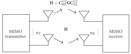
Figure 1 illustrates the MIMO system model in which the
transmitter sends complex symbols from nT antennas and the receiver utilizesnRantennas. The received vector is given by
r=Hb+v, (1)
where b = [b1,b2,. . .,bnT]T is the transmitted vector,v = [v1,v2,. . .,vnR]T is a zero-mean complex white Gaussian
MIMO transmitter
MIMO receiver
nT . .
. nR
. . . H
H=C1RX/2GC1TX/2
Figure1: A schematic block diagram illustrating the MIMO system model.
noise vector, where the elements are independent and iden-tically distributed (i.i.d.) with a varianceσ2 =N
0/2 in each
dimension. The matrix Hdescribes the effect of fading be-tween the two ends of the wireless link, which is assumed to be slow and frequency-nonselective.
The estimated channel matrixHis related to the channel matrixHthrough
H=H+ε, (2)
whereεis annRbynT matrix due to the channel estimation errors. We assume that channel matrixHand the error ma-trixεare uncorrelated and the elements ofεare i.i.d. com-plex Gaussian random variables with zero mean and variance σ2
ε/2 in each dimension [8]. The varianceσε2 indicates the quality of channel estimation and is assumed to be known at the receiver.
2.2. The spatial correlation model
The amplitude of the complex path gainHi,j is assumed to be Rayleigh distributed and the phase is uniform. We can in-troduce spatial correlation via [22]
H=C1RX/2GC1TX/2, (3)
where the elements ofGare i.i.d. complex zero mean Gaus-sian random variables with variance 1/2 in each dimension. The correlation matricesCTX andCRX are real, symmetric,
and reflect the correlation between the elements of a uni-formly spaced antenna array. If the antennas are spaced suf-ficiently apart and there are many scatterers near the trans-mitter or receiver, thenCTXandCRXare given by the identity
matrixI.
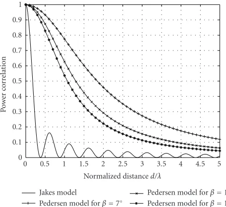
We assume Jakes’ correlation model for the mobile [23], that is, the (i,j)th element is given by CTX(i,j) =
J0(2πdiTX,j/λ), wherediTX,j is the antenna spacing between the ith andjth transmit antenna,λis the wavelength of the car-rier frequency, andJ0is the Bessel function of the zeroth kind.
Figure 2plots the power correlation (the square ofCTX(i,j))
1 0.9 0.8 0.7 0.6 0.5 0.4 0.3 0.2 0.1 0
0 0.5 1 1.5 2 2.5 3 3.5 4 4.5 5 Normalized distanced/λ
P
o
wer
cor
re
lat
ion
Jakes model
Pedersen model forβ=7◦
Pedersen model forβ=10◦ Pedersen model forβ=12◦ Figure2: An illustration of the correlation models used at the mo-bile (Jakes) and base station (Pedersen).
We use the Pedersen correlation model for the base sta-tion, and, if the signals are impinging from broadside, the (i,j)th element ofCRXis adopted from [24]
CRX(i,j)=J0
2πdRX
i,j λ
+ 2 β2
1−exp
−√2π
β
∞
m=1
J2m 2πdRXi,j/λ
β−2+ 2m2 ,
(4)
whereJ2mis the Bessel function of the 2mth kind,diRX,j is the antenna spacing between theith andjth receive antenna, and βis the angular spread measured at the base station. The an-gular spread in a typical outdoor macrocellular urban en-vironment for a carrier frequency of 2.1 GHz is between 7 and 12 degrees [25]. The power correlation (the square of
CRX(i,j)) versus antenna spacing is plotted in Figure 2for
β=7, 10, and 12 degrees.
2.3. Ergodic capacity evaluation with channel estimation errors
The performance of the considered coded MIMO systems will be compared to the ergodic capacity limit. Consequently, in this section, we briefly review the evaluation of this quan-tity and the effects of imperfect channel state information. We can express the rate of transmission of a coded MIMO system asR=nTRmRc(in bits per channel use), whereRmis the modulation rate and the channel coding rateRcis given byk/nwhen ak-bit message is represented as ann-bit coded sequence. Furthermore, the transmitted bit energy-to-noise ratio, which allows comparison to the ergodic channel ca-pacity, is given byEb/N0=P/(2Rσ2), wherePis the average
transmitted power and σ2 = N
0/2 is the noise variance in
each dimension. The ergodic capacity for a MIMO channel with estimation errors is derived in [8] and is given by
CMIMO=E
log2
det
I+ P
2nTσ2HH
H 2σ2 2σ2+σ2
εP
,
(5)
where (•)H is the Hermitian operator andEis the expecta-tion on the random matrixH. Since the channel is assumed to be ergodic, we approximate the statistical expectation in (5) by an average over many realizations ofH.
Figures3and4illustrate the impact of channel estima-tion errors on the channel capacity for (nT,nR)=(2, 10) and (4, 20) antenna configurations (averaged over 100 000 chan-nel realizations) in slow frequency-nonselective uncorrelated and correlated Rayleigh fading channels, respectively. In gen-eral, spatial correlation slightly reduces the ergodic capacity curves from the uncorrelated scenario, whereas the capacity curve for imperfect CSI at the receiver (σ2
ε =0.1 or 10 per-cent) saturates in the high SNR region, while the capacity for perfect CSI at the receiver (σ2
ε = 0) continues to increase. Conversely, at low SNRs, which is our region of interest, the introduction of channel estimation errors slightly shifts the capacity curve to the right with respect to the perfect CSI case.
In terms of SNR performance degradation for actual coded MIMO systems, the capacity results give the perfor-mance degradation (in terms of SNR and/or data rates) be-tween the “best” possible coded system without CSI errors and the “best” possible coded system for given level of CSI errors. If, on the other hand, one considers a specific coded MIMO system, the performance degradation versus CSI er-ror causes the following two limiting cases. For very high values of SNR (σ2 σ2
ε), the channel estimation errors dominate the AWGN noise terms and the BER system per-formance saturates for increasing SNR values. (A potentially low error floor due to the estimation error will occur.) Con-versely, for very low SNR values (σ2σ2
ε), the system per-formance is noise limited, so the CSI error term will result in a minor SNR degradation. Since the channel estimation error causes an additional signal-dependent noise term corrupting the signal (cf. (1) and (2)), a more precise analysis is not el-ementary and strongly depends on the numerical stability of the specific MIMO decoding algorithm(s).
2.4. The transmitter architecture
Figure 5illustrates a schematic block diagram of the
consid-ered MIMO transmitter. The source is assumed to produce independent, equiprobable bits that are passed to the channel encoder, which is a turbo-code consisting of two constituent recursive systematic convolutional encoders as described in [4, 26]. We can describe the encoding process as message symbolsm ∈ {0, 1}k being mapped into codeword symbol of lengthngiven byc=(f1(m),f2(π(m))), where f1(·) and
f2(·) denote the constituent encoders that are separated by
30
25
20
15
10
5
0
Capacit
y
(bits
p
er
ch
annel
u
se)
−10 0 10 20
Eb/N0(dB)
σ2 ε =0%
σ2 ε =10%
(a)
30
25
20
15
10
5
0
Capacit
y
(bits
p
er
ch
annel
u
se)
−10 0 10 20
Eb/N0(dB)
σ2 ε =0%
σ2 ε =10%
(b)
Figure 3: The comparison of the ergodic capacity for slow frequency-nonselective (a) uncorrelated and (b) correlated Rayleigh fading channels with perfect channel state information and 10% channel estimation errors for an (nT,nR)=(2, 10) antenna configuration.
60
50
40
30
20
10
0
Capacit
y
(bits
p
er
ch
annel
u
se)
−10 0 10 20
Eb/N0(dB)
σ2 ε =0%
σ2 ε =10%
(a)
60
50
40
30
20
10
0
Capacit
y
(bits
p
er
ch
annel
u
se)
−10 0 10 20
Eb/N0(dB)
σ2 ε =0%
σ2 ε =10%
(b)
Source Channel
encoder Modulationmapper
Channel interleaver
DeMUX on
nr antennas .
. .
. . .
Figure5: Schematic block diagram of the considered MIMO transmitter.
MIMO signal detector
Channel de-interleaver
MUX from
nT sources
Demapper of demodulator
Estimate of mean and
variance
Channel
decoder Sink ˆ
Hfrom estimator
. . .
. . .
. . .
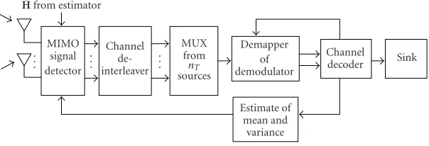
Figure6: Schematic block diagram of the considered MIMO receiver with iterative processing.
symbol. These symbols are demultiplexed ontonT streams, channel interleaved, and transmitted. The role of the chan-nel interleaver and deinterleaver is to break up chanchan-nel fades affecting consecutively transmitted symbols in coded pack-ets.
3. THE RECEIVER ARCHITECTURE
In this section, we first derive a linearly complex MIMO sig-nal detector in the presence of channel estimation errors. The detector tries to separatenT transmitted symbols from the received vectorrand provides soft-decision outputs on the modulation symbols. These soft decisions are then used by a channel decoder, which in our case is a turbo decoder. In addition, a particular low-complexity iterative processing scheme improves the overall system performance. (Figure 6 illustrates the overall schematic block diagram of the itera-tive space-time receiver under consideration.)
3.1. Derivation of the MIMO signal detector
We will assume the discrete-time MIMO channel model from (1). The proposed detector tries to recover channel ob-servations on each transmitted modulation symbol, thus re-ducing the dimensionality of the problem from nR to nT, where for uplink transmission scenarios,nT < nR. The fol-lowing paragraphs outline the general operation of the de-tector and are followed by an illustrative numerical example. As the first step, the estimated channel matrixH is de-composed into two matrices,H =SA, where the matrixAis a diagonal matrix containing the column norms ofH along its main diagonal,
A=diag h1,h2,. . .,hnT, (6) andSis composed of the normalized columns ofH,
S=
h1
h1
,h2
h2
,. . ., hnT
hnT
. (7)
(Please note this decomposition is not related to any of the traditional matrix decompositions used in signal processing, e.g., Cholesky, QR, LU, SVD, etc.)
Consequently, we obtain estimates of the transmitted symbol vectorbby filtering the vector of received observa-tionsrby a bank of parallel filters represented by the matrix
S, that is,
y=SHr=SH H+εb+SHv=RAb +SHεb+n, (8)
whereR =SHSis the antenna correlation matrix. The ele-ments of thenT-by-one vectoryare channel observations on the transmitted vectorbwhich are corrupted by co-antenna interference due toRA, as well as the channel estimation er-ror inSHεband the filtered noisen. The jth element ofyis given by
yj=Aj,jbj+ nT
k=1
k=j
Rj,kAk,kbk+ SHεb
j+nj, (9)
where Rj,k = R∗k,j = sHjsk (conjugate is denoted by (•)∗),
Rj,j =1, and the filtered noise elementsnjhave zero means and covariance matrix 2σ2R.
In order to compute the likelihood (soft decision) for the transmitted symbolbjbeing thelth modulation symbol, that is,P(yj|bj =Ql), we approximate in (9) the sum of the co-antenna interferencenT
k=1
k=j
Rj,kAk,kbk, the channel estimation
error (SHεb)
j, and the filtered noisenjas a two-dimensional Gaussian random variable. As shown in Appendix A, the meanµjof this Gaussian random variable is given by
µj=
nT
k=1
k=j
E Rj,kAk,kQ
,
nT
k=1
k=j
ERj,kAk,kQ
and covariance matrixKjof this complex Gaussian random variable is
Kj(1, 1)= nT
k=1
k=j
E Rj,kAk,kQ 2
!
− E Rj,kAk,kQ
2
+σ2+σε2 2 ,
Kj(2, 2)= nT
k=1
k=j
E Rj,kAk,kQ 2
!
− ERj,kAk,kQ 2+σ2+σ
2
ε 2,
Kj(1, 2)=Kj(2, 1)
=
nT
k=1
k=j
E Rj,kAk,kQ
Rj,kAk,kQ
− E Rj,kAk,kQ E
Rj,kAk,kQ
, (11)
where {•}and{•}denote the real and imaginary parts andEis the expectation on the discrete random variableQ, which can be one ofMpossible modulation symbols.
Finally, we can express the likelihood for the transmitted symbol from the jth antennabj being the lth modulation symbolQlas follows:
p yj|bj=Ql
=exp
"
−(1/2) xj−µj−Aj,jql
K−j1 xj−µj−Aj,jql
T#
2π$det Kj
,
(12)
where xj = [ {yj},{yj}]T,ql = [ {Ql},{Ql}]T, and (•)Tis transpose operator. The following example illustrates the numerical operations of the detector.
Example1. Consider an (nT,nR)=(2, 4) system, where the transmitter sends a BPSK symbol vectorb=[1,−1] and the channel matrix is given by
H=
0.5 + 0.5i 0.5−0.5i 1 + 1i 1−1i
−1 1
−1i −1i
. (13)
Assume that the receiver estimates the channel with an es-timation error of σ2
ε = 0.1 and that the channel matrix is estimated as
H=
0.70 + 0.42i 0.28−0.64i 0.97 + 0.68i 1.09 + 0.73i
−0.84 + 0.10i 0.96−0.47i
−0.31−1.30i 0.30−0.80i
(14)
and the Gaussian noise variance in each dimension isσ2=1.
The received vectorrwas observed to be
r=
−0.28 + 0.45i
−1.14−0.67i
−1.66−0.10i
−1.32−0.04i
. (15)
Step 1 (matrix decomposition). The detector decomposes the channel matrix into the two submatrices according to (6) and (7):
A=
2.13 0 0 2.02
,
S=
0.33 + 0.20i 0.14−0.32i 0.46 + 0.32i 0.54 + 0.36i
−0.39 + 0.05i 0.47−0.23i
−0.14−0.61i 0.15−0.40i
.
(16)
Step 2 (acquiring channel observations). We filter the re-ceived vector rby the matrixSto lower the dimensionality of the problem (fromnR=4 tonT =2) and acquire channel observations on the transmitted symbols contained iny. The channel observation vectory(using (8)) is given by
y=
0.13−0.42i
−1.97−0.94i
. (17)
Note that this reduction in dimensionality is interesting for the case of large number of receive antennas (at the base sta-tion) when compared to the number of transmit antennas (at the mobile), for example, practical prototype systems with nR=60 have already been explored, as mentioned in [21].
Step 3 (computing statistics for the Gaussian approxima-tion). The co-antenna correlation matrixR = SHSis given by
R=
1 0.37 + 0.08i 0.37−0.08i 1
, (18)
and hence the statistics for the Gaussian approximation for the co-antenna interference, channel estimation error, and the filtered noise from (10) and (11) for the first transmit antenna are
µ1=0,
K1=
1.65 0 0 1.13
,
(19)
where the mean vectorµ1andK1(1, 2),K1(2, 1) are zero as
Step4 (determination of the soft decisions). Using (12), the likelihoods for the symbol from the first transmit antenna are given byP(y1|b1 = −1) = 0.022 andP(y1|b1 = 1) =
0.033 repeating the above calculation for the second transmit antenna,P(y2|b2 = −1)=0.077 andP(y2|b2=1)=0.006.
(Please note that these likelihoods are not normalized asa posteriori probabilities would be.)
3.2. Turbo decoding and iterative processing
The demapper inFigure 6translates the soft decisions of the detector intoaposteriori probabilities on the codeword sym-bols. For instance, the estimate for the pth codeword bit in the jth modulation stream is given by
Λp=P cp=0|yj,p
P cp=1|yj,p
=
Ql∈{M−QAM|cp=0}P yj,p|bj=Ql
P bj=Ql
Ql∈{M−QAM|cp=1}P yj,p|bj=Ql
P bj=Ql. (20)
The estimatesΛpare assumed to be the channel observations on the bits of codeword symbols.
In theith iteration, the iterative loop between the decoder and demapper can be formally described as
wi1,wi2
=φ u,zi−1 1,zi−21
−zi−11,zi−2 1
,
zi2,xi2
=ϕ2 w2i,xi−1 1
−xi−11,
zi
1,xi1
=ϕ1 wi1,xi2
−xi
2,
(21)
where the soft decision demapper and decoding functions are represented byφandϕ1,ϕ2, respectively. The vectorsu
andwi1,wi2denote the soft outputs of the linear detector and
the demapper, respectively inFigure 6. The decoding func-tionsϕ1 andϕ2 evaluate logarithmic arrays ofa posteriori
probabilities for message symbols and codeword symbols of the constituent encoders of the turbo-code. The extrinsic in-formation vectors on the codeword symbols (zi1andzi2) and
on the message bits (x1i andxi2) are initially (fori = 0) set
to a constant and are treated as independent coordinatewise observations of these symbols or bits, so that, for instance, P(mj =k|x) is proportional to exp(xk,j). The decisions on the message symbols are formed by thresholding outputs of the first decoderϕ1(wi1,xi2) after each iteration.
Turbo equalization was first proposed in [27] and in-volves the recomputation of the probabilities on the trans-mitted modulation symbols from theaposteriori probabil-ities on the codeword symbols. These computed probabili-ties on the modulation symbols become the extrinsic infor-mation for the detector and hence will result in better esti-mates on the codeword symbols. Although this method may be feasible in single-antenna systems, the transmitted signal vector constellation quickly becomes too large for a coded MIMO system as it increases asMnT forM-ary modulation withnT antennas. In the approach under consideration, we reassemble the codeword symbol probabilities into probabil-ities on the modulation symbolsP(bj =Ql) and recompute
the mean vector and covariance matrix of the Gaussian ap-proximation using (10) and (11). As the system iterates, the mean of the co-antenna interference will approach the true interference value and its variance becomes zero, thus the ef-fect of the interference is removed from the received symbol.
4. SIMULATION RESULTS
In this section, we present simulation results of the proposed linear-complexity detector in two uplink coded MIMO systems. These simulation results are evaluated for slow, frequency-nonselective Rayleigh fading channels when per-fect and imperper-fect channel state information is available at the receiver only. As discussed in the introduction, we con-sider the uplink transmission scenario where it is possible to have a large number of receive antennas, for example, 10 and 20. The message block size was chosen to be 32000 bits and the channel code is a rate 1/2 turbo-code, which is composed of two eight state quaternary recursive systematic encoders (rate 2/3) adopted from [26]. The turbo encoder contains a symmetricS-rand interleaver [28], whereS=80. The coded bits are mapped into 16-QAM modulation symbols, whose lookup table has been adopted from [29]. We use the spatial correlation model, described in Section 2.2, where the an-tenna spacing at the mobile and base station is assumed to be λ/2 andλ, respectively, and the angular spreadβis assumed to be 10 degrees. The ergodic capacity limits are evaluated numerically by averaging over 1 million channel realizations and the variance of the estimation errorsσ2
ε is set to be 10 percent. The turbo decoder in the receiver performs 10 de-coding iterations and uses the BCJR algorithm [30] in the constituent decoders.
Figures7and8compare the performance of the coded MIMO system utilizing the proposed detector (of linear complexity) to the T-BLAST system [3] (of cubic MIMO sig-nal detection complexity) for the (2, 10) and (4, 20) antenna configurations in an uncorrelated Rayleigh fading channel with perfect CSI at the receiver. Both systems operate at equivalent rates (the T-BLAST using a 16-PSK modulation), use the same antenna setups and perform 10 decoding iter-ations. Our proposed system outperforms the T-BLAST sys-tem by about 10 dB in both cases at a bit error rate of 10−5
and achieves performance within 1.5 dB of the ergodic ca-pacity limit.
Figure 9 illustrates the performance of the considered
100
10−1
10−2
10−3
10−4
10−5
−8 −6 −4 −2 0 2 4
Eb/N0(dB)
BER
T-BLAST fornT=2 andnR=10
Proposed coded MIMO system fornT=2 andnR=10 Capacity limit (nT,nR)=(2, 10),R=4 bits/channel use Figure 7: Performance comparison illustrating the 10 dB coding gain between the proposed coded MIMO system and the T-BLAST architecture [3] for (nT,nR)=(2, 10) antennas. Simulation results are shown after iterations 1, 2, 4, 8, and 10 on an uncorrelated Rayleigh fading channel with perfect CSI at the receiver only.
100
10−1
10−2
10−3
10−4
10−5
−10 −8 −6 −4 −2 0
Eb/N0(dB)
BER
T-BLAST fornT=4 andnR=20
Proposed coded MIMO system fornT=4 andnR=20 Capacity limit (nT,nR)=(4, 20),R=8 bits/channel use Figure 8: Performance comparison illustrating the 10 dB coding gain between the proposed coded MIMO system and the T-BLAST architecture [3] for (nT,nR)=(4, 20) antennas. Simulation results are shown after iterations 1, 2, 4, 8, and 10 on an uncorrelated Rayleigh fading channel with perfect CSI at the receiver only.
have a larger impact than in the uncorrelated case. That is, the performance of the coded MIMO system with (nT,nR)= (2, 10) and (4, 20) antennas is within 2.1 and 2.8 dB of the er-godic capacity limit, respectively. These systems perform 1.2 and 1.6 dB worse for (nT,nR)=(2, 10) and (4, 20) antenna
100
10−1
10−2
10−3
10−4
10−5
−16 −15 −14 −13 −12 −11 −10 −9 −8 −7 −6
Eb/N0(dB)
BER
(2, 10): perfect CSI
Capacity limit for (2, 10), perfect CSI (2, 10): 10% error variance
Capacity limit for (2, 10), 10% error variance (4, 20): perfect CSI
Capacity limit for (4, 20), perfect CSI (4, 20): 10% error variance
Capacity limit for (4, 20), 10% error variance
Figure 9: Performance of the proposed MIMO system in a slow frequency-nonselective uncorrelated Rayleigh fading channel for (nT,nR)=(2, 10) and (4, 20) antennas.
configurations, respectively, when compared to the corre-sponding systems which have perfect CSI at the receiver. An estimation error variance of 10% represents a large value and the works in [9,10,11] indicate that the error variance is usually much smaller, that is, lower than 1 percent. In these scenarios, the performance loss due to channel estimation er-rors in our considered coded MIMO system is expected to be smaller, if not negligible.
Figure 11illustrates reduction of the co-antenna
interfer-ence during the iterative decoding process for different CSI/ correlation scenarios and values of SNR. In all four cases, at low SNRs, the variance does not converge to zero, whereas for slightly higher SNRs, the variance reaches zero in less than ten iterations. In correlated channels, the initial variance of the co-antenna interference is about three times larger than in the uncorrelated case. Furthermore, for the variance of the co-antenna interference to converge, channel estimation er-rors require an additional SNR increase of 1 dB and 1.6 dB in the uncorrelated (Figures11a,11b) and correlated fading (see Figures11c,11d) scenarios, respectively.
5. ANALYSIS OF THE PROPOSED DETECTOR
100
10−1
10−2
10−3
10−4
10−5
−14 −13 −12 −11 −10 −9 −8 −7 −6 −5
Eb/N0(dB)
BER
(2, 10): perfect CSI
Capacity limit for (2, 10), perfect CSI (2, 10), 10% error variance
Capacity limit for (2, 10), 10% error variance (4, 20): perfect CSI
Capacity limit for (4, 20), perfect CSI (4, 20): 10% error variance
Capacity limit for (4, 20), 10% error variance
Figure 10: Performance of the proposed system in a slow frequency-nonselective correlated Rayleigh fading channel for (nT,nR)=(2, 10) and (4, 20) antennas.
are loose by about 2 dB at low SNRs [31]. The other classes of techniques are either limited to low-density parity-check codes [32] or provide only the SNR value at which the turbo decoder starts to converge [33]. Consequently, as an initial step towards the desired BER performance analysis, this sec-tion derives closed-form expressions for the proposed detec-tor’s soft-output statistics and symbol error rates after the de-tector.
5.1. Analysis of co-antenna interference in Rayleigh fading channels
To better characterize the co-antenna interference, we will determine the mean and variance of the column norms and correlations between the normalized columns of thenR by nT random channel matrixH. In the following, we assume σ2
ε = 0, that is, perfect CSI is available at the receiver and drop the use of the “hat” symbol. To permit mathematical tractability, we assume the base station antennas are corre-lated and mobile antennas are uncorrecorre-lated.
Claim 1. The jth column norm of H Aj,j is a chi ran-dom variable withnR degrees of freedom, mean √2Γ(nR/2 + 0.5)/Γ(nR/2) ≈ √nR, and variance of σ2
Aj,j = 2Γ(nR/2 + 1)/Γ(nR/2)−µ2
Aj,j ≈ 1/2for reasonable values of nR,(nR < 100), an angular spreadβof ten degrees, and antenna spacing at the receiver given byλ.
Justification ofClaim 1
Using (3), the norm of thejth column norm ofHAj,jis given by
Aj,j=
$ hHjhj=
% gHj C1RX/2
H
C1RX/2gj
=$gHj CRXgj=
$
gHjVΛVTgj=$eH jej,
(22)
where in the fourth step we performed the eigenvalue de-composition on the real and symmetric matrixCRX
result-ing in the real orthogonal and diagonal matrices VandΛ, respectively. Thelth element ofejis a realization of a com-plex Gaussian random variable with zero mean and variance Λl,l/2 in the real and imaginary dimensions,l=1, 2,. . .,nR.
Further expanding the last line of (22),
Aj,j=
& ' ' (nR
l=1
"
ej,l
2
+ ej,l
2#
= & ' ' (nR
l=1
Wl2+ nR
l=1
Xl2,
(23)
whereWlandXlare independent and Gaussian distributed with zero mean and varianceΛl,l/2,l =1, 2,. . .,nR.
Conse-quently, the random variableA2j,jis chi-squared distributed with 2nR degrees of freedom (as it is the sum of 2nR chi-squared random variables [34]), and its mean and variance are given by
µA2 j,j =
nR
l=1
µW2 l +
nR
l=1
µX2 l =2
nR
l=1
Λl,l 2 ,
σ2
A2 j,j =
nR
l=1
σ2
W2 l +
nR
l=1
σ2
X2 l =2
nR
l=1
Λ2
l,l 2 .
(24)
Since by (4), the elements of CRX depend on the random
parameter β(angular spread measured at the receiver), the quantities in (24) are random variables.
For the specific case ofβ =10 degrees and an antenna spacing at the receiver isλ, the mean and the variance in (24) become approximatelynRand 2nR, respectively. Hence,Aj,j is a chi random variable withnRdegrees of freedom that can be expressed as follows:
Aj,j=
& ' ' (nR
l=1
Θ2
l, (25)
whereΘlare i.i.d. Gaussian random variables with zero mean and unit variance for l = 1, 2,. . .,nR. The mean of Aj,j is given by µAj,j =
√
2Γ(nR/2 + 0.5)/Γ(nR/2) and its variance is σ2
Aj,j = 2Γ(nR/2 + 1)/Γ(nR/2)−µ
2
4 3.5 3 2.5 2 1.5 1 0.5 0
V
ar
ianc
e
in
re
al
dimension
0 2 4 6 8 10 Iteration #
Eb/N0= −10 dB
Eb/N0= −9.5 dB
Eb/N0= −8.75 dB (a)
4 3.5 3 2.5 2 1.5 1 0.5 0
V
ar
ianc
e
in
re
al
dimension
0 2 4 6 8 10 Iteration #
Eb/N0= −9 dB
Eb/N0= −8.5 dB
Eb/N0= −7.75 dB (b)
10 9 8 7 6 5 4 3 2 1 0
V
ar
ianc
e
in
re
al
dimension
0 2 4 6 8 10 Iteration #
Eb/N0= −8.75 dB
Eb/N0= −7.75 dB
Eb/N0= −6.75 dB (c)
10 9 8 7 6 5 4 3 2 1 0
V
ar
ianc
e
in
re
al
dimension
0 2 4 6 8 10 Iteration #
Eb/N0= −7.125 dB
Eb/N0= −6.125 dB
Eb/N0= −5.125 dB (d)
Figure11: Reduction of the co-antenna interference during the iterative decoding process for the (nT,nR)=(4, 20) antenna coded MIMO system on slow frequency-nonselective Rayleigh fading channels: (a) uncorrelated fading and perfect CSI, (b) uncorrelated fading and im-perfect CSI (10% error variance), (c) correlated fading and im-perfect CSI, and (d) correlated fading and imim-perfect CSI (10% error variance).
Claim 2. The (j, k)th element of the antenna correlation ma-trix Rj,k is a zero-mean complex Gaussian random variable with variance1/nR in each dimension for an angular spread βof ten degrees and an antenna spacing at the receiver ofλ.
Justification ofClaim 2
Assuming the same parameters as before for the spatial cor-relation, that is,β=100, and the antenna spacing at the
re-ceiver given byλ, we can express the correlation between the jth andkth normalized columns ofHas
Rj,k=
hH jhk
hjhk≈
hH jhk nR
=g
H j C1RX/2
H
C1RX/2gk
nR =
gH jCRXgk
nR ,
(26)
where the column norms are approximated by √nR, as the variance is reasonably small (approximately 1/2). Using the eigenvalue decomposition onCRX,
Rj,k≈
gH
jVΛVTgk nR =
eH jek nR
= 1
nR
nR
l=1
Wl+ nR
l=1
Xl+i
nR
l=1
Yl+ nR
l=1
Zl
,
(27)
where Wl,Xl,Yl, and Zl are independent Gaussian prod-uct variables with zero mean and variance Λ2l,l/4 for l =
1, 2,. . .,nR. SincenR
l=1Λ2l,l/4≈nR/2, we can apply the central
limit theorem on each summation, and hence express Rj,k as a complex Gaussian random variable with zero mean and variance 1/nRin each dimension.
Finally, the uncorrelated fading scenario is a special case of the correlated case, where CRX = I. Hence, Wl andXl
in (23) are i.i.d. zero-mean Gaussian random variables with variance 1/2 forl =1, 2,. . .,nR. Therefore, the norm of the jth column ofH,Aj,j, is a chi random variable with 2nR de-grees of freedom and its mean isµAj,j =Γ(nR+0.5)/Γ(nR) and variance isσ2
Aj,j=Γ(nR+ 1)/Γ(nR)−µ
2
Aj,j. The mean can still be approximated as√nRand, for reasonably largenR(e.g., up to 100), the variance ofAj,jis close to 1/4. Similarly,Wl,Xl, Yl, andZlin (27) are i.i.d Gaussian product random variables with zero mean and variance 1/2 forl = 1, 2,. . .,nR. Using the central limit theorem, we can approximate the summa-tions in the real and imaginary dimensions ofRj,k in (27) as a Gaussian random variable with zero mean and variance 2nR/(4n2R)=1/(2nR).
5.2. Performance analysis of the MIMO detector
We consider the average and approximate probability of sym-bol error of the proposed detector for the cases of perfect and imperfect CSI at the receiver in slow frequency-nonselective uncorrelated and correlated Rayleigh fading channels. The average probability of symbol error considers the full corre-lation model (CTX andCRX), while (to permit
Furthermore, the transmitted symbols from each antenna are assumed to be equiprobable and independent of transmitted symbols from other antennas.
Claim 3. Let the channel observation vector in the presence of channel estimation errors be given byy=RAb) +n, whereR)=
SHS. Then the probability of symbol error conditioned on the estimated channelH for the first transmit antenna is given by
Pdemod1 error|H
= 4
MnT
×
M
l2=1 M
l3=1
· · ·
M
lnT=1
1−Q
{
D}−R)1,1A1,1B
σ
×Q
{
D}−R)1,1A1,1B
σ
+
√
M−22 MnT
×
M
l2=1 M
l3=1
· · ·
M
lnT=1
1−
1−2Q
{
D}+R)1,1A1,1B
σ
×
1−2Q
{
D}+R)1,1A1,1B
σ
+4
√
M−2 MnT
×
M
l2=1 M
l3=1
· · ·
M
lnT=1
1−Q
− {
D} −R)1,1A1,1B
σ
×
1−2Q
{
D}+R)1,1A1,1B
σ
,
(28)
whereD = −nT
k=2R)1,kAk,kQlk is the co-antenna interference
for j = 1transmit antenna and for the case of perfect CSI at the receiver,R)=SHS, andR)
1,1=1.
(Note that for a time-varying channel, the average prob-ability of symbol error can be determined by averaging the above expression over many channel realizations as the chan-nel is assumed to be stationary and ergodic.)
Justification ofClaim 3
We can reexpress the channel observation vectoryfrom (8) as
y=RAb) +n, (29)
whereH=SA,R)=SHS,n=SHv, andy
1is given by
y1=R)1,1A1,1b1+
nT
k=2
)
R1,kAk,kbk+n1, (30)
whereR)1,1is a loss factor corresponding to the imperfect CSI
being available at the receiver. The probability of symbol er-ror conditioned on the estimated channel matrix is given by
P1demod error|H
=
M
l=1
Pb1=Ql
Py1∈Zl|b1=Ql
, (31)
where the minimum distance decision regionZlcorresponds to thelth QAM symbolQl. If we further conditionP[y1 ∈
Zl|b1 =Ql] on the remaining transmit antennas, that is, let
bk =Qlk,k = 2, 3. . .,nT, then the co-antenna interference term in (30) becomes a deterministic quantity. Therefore, the QAM symbol transmitted from the first antennab1is only
corrupted by additive Gaussian noise and hence assuming the real and complex parts of y1are independent the
prob-ability of error in (31) is given by the weighted sum of the probability of error whenb1=Qlis a corner, middle, or side
point of the constellation,
Pcornere =1−P
{n1}> {D} −R)1,1A1,1B
×P{n1}>{D} −R)1,1A1,1B
,
Pmiddlee =1−P
{D}−R)1,1A1,1B < {n1}< {D}+R)1,1A1,1B
×P{D}−R)1,1A1,1B <{n1}<{D}+R)1,1A1,1B
,
Pe
side=1−P
{n1}< {D}+R)1,1A1,1B
×P{D}−R)1,1A1,1B <{n1}<{D}+R)1,1A1,1B
, (32)
whereD= −nT
k=2R)1,kAk,kQlkis the co-antenna interference for the first (j =1) transmit antenna and {n1},{n1}are
the real and imaginary components of the noisen1.
We can evaluate (31) by using (32) and theQ-function [36]
Pdemod
1 error|H
= 4
MnT
×M
l2=1 M
l3=1
· · · M
lnT=1
1−Q
{
D} −R)1,1A1,1B
σ
×Q
{
D}−R)1,1A1,1B
σ
+
√
M−22 MnT
×
M
l2=1 M
l3=1
· · ·
M
lnT=1
1−
1−2Q
{
D}+R)1,1A1,1B
σ
×
1−2Q
{
D}+R)1,1A1,1B
σ
+4
√
M−2 MnT
×
M
l2=1 M
l3=1
· · ·
M
lnT=1
1−Q
− {
D} −R)1,1A1,1B
σ
×
1−2Q
{
D}+R)1,1A1,1B
σ
If we have perfect CSI at the receiver, then R) = SHS and
)
R1,1 = 1. For a time-varyingH, we can average the symbol
error probability in (33) over many channel realizations as the channel is assumed to be stationary and ergodic. In the following, we derive the approximate performance of the de-tector as a closed-form expression.
Claim 4. Let the channel observation vector in the presence of channel estimation errors be given byy=RAb) +n, whereR)=
SHS. Then the approximate probability of symbol error forj= 1transmit antenna is given by
Pdemod 1 (error)
≈ 4
MnT
M
l2=1 M
l3=1
· · ·
M
lnT=1
1−Q
−$R)1,1√nRB
σ2 CAI+σ2
2 + √
M−22 MnT
×
M
l2=1 M
l3=1
· · ·
M
lnT=1
1−
1−2Q
−$R)1,1√nRB
σ2 CAI+σ2
2 +4 √
M−2 MnT
×
M
l2=1 M
l3=1
· · ·
M
lnT=1
1−Q
−$R)1,1√nRB
σ2 CAI+σ2
×
1−2Q
−$R)1,1√nRB
σ2 CAI+σ2
, (34)
where R)1,1 is the average loss factor due to imperfect CSI at
the receiver and the variance of the co-antenna interference in each dimension is given by σ2
CAI =
nT
k=2Qlk2/2 and
σCAI2 =
nT
k=2Qlk2for the uncorrelated and correlated fading
scenario, respectively. For the case of perfect CSI at the receiver,
)
R=SHSandR)
1,1=1.
Justification ofClaim 4
As mentioned earlier, to permit mathematical tractability, we assume spatial correlation at the base station only. Without loss of generality, we consider the j = 1 transmit antenna, where the channel observation is given in (30) and the corre-sponding probability of symbol error is given by
P1demod(error)=
M
l=1
Pb1=Ql
Py1∈Zl|b1=Ql
. (35)
If we conditionP[y1∈Zl|b1=Ql] on the remaining
trans-mit antennas, that is, let bk = Qlk, k = 2, 3,. . .,nT, then the co-antenna interference (CAI) term in (30) will be de-pendent on two random variablesAk,k andR)1,k. Using the results of the previous section, we can approximate Ak,k, k = 1, 2,. . .,nT, by its mean√nR as its variance is small (1/4 or 1/2) and since the elements of ε are much smaller than the elements of the channel matrix, the correlation co-efficientR)1,k (k = 1) will be assumed to remain as a zero-mean complex Gaussian random variable with a variance of
1/(2nR) and 1/nRin each dimension for the uncorrelated and correlated fading scenarios, respectively. Hence, the CAI term is a complex Gaussian random variable with zero mean and varianceσCAI2 =
nT
k=2Qlk
2/2 andσ2 CAI =
nT
k=2Qlk
2 in
each dimension and the probability of error in (35) is given by the classical expression for a QAM symbol corrupted by additive Gaussian noise. As mentioned previously, the prob-ability of symbol error is the weighted sum of the three ex-pressions for the probability of error forb1=Qlis a corner,
middle, or side point of the constellation
Pe
corner=1−P
{n1}>−R)1,1A1,1B
!
P{n1}>−R)1,1A1,1B
!
,
Pmiddlee =1−P
−R)1,1A1,1B < {
n1}<R)1,1A1,1B
!
×P−R)1,1A1,1B <{
n1}<R)1,1A1,1B
!
,
Pe
side=1−P
{n1}<R)1,1A1,1B
!
×P−R)1,1A1,1B <{
n1}<R)1,1A1,1B
!
,
(36)
where we assumed the real and complex parts of y1are
in-dependent andn1 is the sum of the Gaussian noisen1and
the CAI term ( andrefer to the real and imaginary com-ponents). Since R)1,1 is random variable with an unknown
density function, we can approximate it by its value averaged over many channel realizationsR)1,1, where for instance,R)1,1
is equal to 0.95 for an estimation error variance of 10% (av-eraged over 100 000 channel realizations). Therefore, the ap-proximate probability of error for the first transmit antenna using (36) and theQ-function [36] is given by
P1demod(error)
≈ 4
MnT
M
l2=1 M
l3=1
· · ·
M
lnT=1
1−Q
−$R)1,1√nRB
σ2 CAI+σ2
2 + √
M−22 MnT
×
M
l2=1 M
l3=1
· · ·
M
lnT=1
1−
1−2Q
−$R)1,1√nRB
σ2 CAI+σ2
2 +4 √
M−2 MnT
×
M
l2=1 M
l3=1
· · ·
M
lnT=1
1−Q
−$R)1,1√nRB
σ2 CAI+σ2
×
1−2Q
−$R)1,1√nRB
σ2 CAI+σ2
, (37)
where for perfect CSI at the receiverR)=SHSand henceR)
1,1
=1 in (37).
5.3. Numerical results
0.03
0.025
0.02
0.015
0.01
0.005
0
No
rm
al
iz
ed
o
cc
u
rr
en
ce
ra
te
0 2.5 5 7.5 10 Norm of the first column in the channel matrix
Derived density function Simulated density function
(a)
0.03
0.025
0.02
0.015
0.01
0.005
0
No
rm
al
iz
ed
o
cc
u
rr
en
ce
ra
te
0 2.5 5 7.5 10 Norm of the first column in the channel matrix
Derived density function Simulated density function
(b)
Figure12: The derived and simulated density functions ofA1,1for (nT,nR)=(4, 20) antennas in slow frequency-nonselective (a)
uncorre-lated and (b) correuncorre-lated Rayleigh fading channels.
and correlated Rayleigh fading channels. As mentioned in
Section 5.1, we will only consider spatial correlation at the
base station, that is, using Pedersen’s model (4) with an an-tenna spacing ofλand an angular spread ofβ=10◦.
In Figures 12a and 12b, we plot the derived chi den-sity function of A1,1 and compare it against the simulated
density function. In both the uncorrelated and correlated cases, the mean is approximately 4.5 (≈√nR) and the vari-ance is 1/4 and 1/2, respectively, which agrees with their predicted values from Section 5.1. In Figures13aand13b, we plot the derived and simulated density functions of the real component of R1,2 for 1 million channel realizations.
In Section 5.1, we showed that by the central limit
theo-rem, the derived density function is approximately Gaussian and this is confirmed by the simulated density function. In both uncorrelated and correlated cases, the simulated den-sity function has zero mean and variance, 0.025 and 0.05 re-spectively, which agrees with the derived mean and variance. Since 99% of all correlation coefficient values lie in the range [−3/.2nR, 3/.2nR]=[−0.47, 0.47] for the uncorrelated case and [−3/√nR, 3/√nR]=[-0.67, 0.67] for the correlated case, we observe that high correlations are possible between trans-mit antennas (>15%).
5.4. Performance results of the detector
We consider the performance of the linear MIMO signal detector in slow frequency-nonselective uncorrelated and correlated Rayleigh fading channels. The spatial correlation model is as described inSection 2.2with an antenna spacing ofλ/2 andλat mobile and base station, respectively and the
angular spreadβis assumed to be 10 degrees. Figures14and 15illustrate the average symbol error rate of the MIMO sig-nal detector averaged over 100 000 channel realizations (us-ing (33)) and the corresponding approximate symbol error rate (using (37)) for (nT,nR)=(2, 10) and (4, 20) antennas, respectively using a 16-QAM symbol constellation with per-fect and imperper-fect channel state information (σ2
ε =10%) be-ing available at the receiver. In the uncorrelated cases (Fig-ures14aand15a), there is a close match between the approx-imate and average performance. However, in the correlated cases (Figures14band15b), there exists a small difference be-tween the approximate and average symbol error rate as the approximate performance does not include the spatial corre-lation between transmit antennas. For comparison, the per-formance of the optimal detector is also shown for the same system parameters.
Although the proposed detector is co-antenna interfer-ence limited at high SNRs, it only performs slightly worse than the exponentially complex optimal detector at very low SNRs, for example,−5 to−10 dB, which is the region cor-responding to the performance of the coded MIMO systems as shown in Figures9and10. Furthermore, Figures14and 15illustrate that the performance of the detector is robust to channel estimation errors.
6. CONCLUSION
0.03
0.025
0.02
0.015
0.01
0.005
0
No
rm
al
iz
ed
o
cc
u
rr
en
ce
ra
te
−1 −0.5 0 0.5 1 The real part of the correlation coefficientR1,2
Derived density function Simulated density function
(a)
0.04 0.035 0.03 0.025 0.02 0.015 0.01 0.005 0
No
rm
al
iz
ed
o
cc
u
rr
en
ce
ra
te
−1 −0.5 0 0.5 1 The real part of the correlation coefficientR1,2
Derived density function Simulated density function
(b)
Figure13: The derived and simulated density functions of {R1,2}for (nT,nR)=(4, 20) antennas in slow frequency-nonselective (a) uncor-related and (b) coruncor-related Rayleigh fading channels.
100
10−1
Sy
m
b
o
l
er
ro
r
ra
te
−15 −10 −5 0
Eb/N0per antenna (dB) Approximate,σ2
ε =0% Average,σ2
ε =0% Approximate,σ2
ε =10%
Average,σ2 ε =10% Optimal,σ2
ε =0% Optimal,σ2
ε =10% (a)
100
10−1
Sy
m
b
o
l
er
ro
r
ra
te
−15 −10 −5 0
Eb/N0per antenna (dB) Approximate,σ2
ε =0% Average,σ2
ε =0% Approximate,σ2
ε =10%
Average,σ2 ε =10% Optimal,σ2
ε =0% Optimal,σ2
ε =10% (b)
100
10−1
Sy
m
b
o
l
er
ro
r
ra
te
−15 −10 −5
Eb/N0per antenna (dB) Approximate,σ2
ε =0% Average,σ2
ε =0% Approximate,σ2
ε =10%
Average,σ2 ε =10% Optimal,σ2
ε =0% Optimal,σ2
ε =10% (a)
100
10−1
Sy
m
b
o
l
er
ro
r
ra
te
−15 −10 −5
Eb/N0per antenna (dB) Approximate,σ2
ε =0% Average,σ2
ε =0% Approximate,σ2
ε =10%
Average,σ2 ε =10% Optimal,σ2
ε =0% Optimal,σ2
ε =10% (b)
Figure15: Performance analysis of the proposed and optimal detector for (nT,nR)=(4, 20) antenna system in slow frequency-nonselective (a) uncorrelated and (b) correlated Rayleigh fading channels.
most practical scenarios, channel estimation errors occur at the receiver, especially in the uplink transmission scenarios due to power limitations at the mobile. In this paper, we gen-eralized the linear detector proposed in prior work [1, 2] to accommodate channel estimation errors and considered its robustness in coded MIMO systems on slow frequency-nonselective correlated Rayleigh fading channels.
We consider an uplink transmission scenario, where it is feasible to have a larger number of receive antennas at the base station than the number of transmit antennas at the mobile. In an uncorrelated Rayleigh fading channel with per-fect CSI at the receiver, the proposed detector in the turbo-coded MIMO system outperforms the T-BLAST system [3] by about 10 dB while performing within 1.5 dB of the ergodic capacity limit (at a bit error rate of 10−5) for the (nT,nR)=(2,
10) and (4, 20) antenna configurations. Furthermore, for a channel estimation error variance of 10%, we demonstrated that the turbo-coded MIMO system with (nT,nR)=(2, 10) (4 bits per channel use) and (4, 20) antennas (8 bits per channel use) operates within 1.6 dB of the ergodic capacity limit at a bit error rate of 10−5 for uncorrelated channels,
whereas in spatially correlated channels and the same esti-mation error variance, the performance of the (nT,nR)=(2, 10) and (4, 20) antenna systems is within 2.1 dB and 2.8 dB of the ergodic capacity limit at a bit error rate of 10−5,
respec-tively.
We characterized the co-antenna interference at the out-put of the proposed detector through density functions of the column norm and the correlation between the columns of the random channel matrixH. By doing so, we determined
the approximate closed-form expressions for the perfor-mance of the detector and compared this to an average based on many channel realizations. Although the linearly complex detector was found to be co-antenna interference limited at high SNRs, at very low SNRs, that is,−5 to−10 dB, which is the region corresponding to the coded MIMO system per-formance, it performs only marginally worse than the expo-nentially complex optimal detector. Furthermore, the linear detector is robust to channel estimation errors in correlated and uncorrelated Rayleigh fading channels.
Future work includes a BER performance analysis of the coded MIMO system that features the proposed detector and turbo decoder, extending the system to frequency-selective channels and a multiuser uplink scenario.
APPENDICES
A. APPROXIMATING THE OUTPUT STATISTICS OF THE PROPOSED MIMO SIGNAL DETECTOR
We would like to analyze the output statistics of the MIMO signal detector from Section 3.1. The jth element of the channel observation vectory(from (9)) is given by
yj=Aj,jbj+
nT
k=1
k=j
Rj,kAk,kbk+ SHεb
j+nj, (A.1)
![Figure 7: Performance comparison illustrating the 10 dB codinggain between the proposed coded MIMO system and the T-BLASTarchitecture [3] for (nT,nR) = (2,10) antennas](https://thumb-us.123doks.com/thumbv2/123dok_us/1137796.1142723/8.600.55.287.71.274/figure-performance-comparison-illustrating-codinggain-proposed-blastarchitecture-antennas.webp)
