R E S E A R C H
Open Access
A high-order finite difference scheme for
a singularly perturbed reaction-diffusion
problem with an interior layer
Zhongdi Cen
1,2, Anbo Le
2*and Aimin Xu
2*Correspondence:
2Institute of Mathematics, Zhejiang
Wanli University, Ningbo, China Full list of author information is available at the end of the article
Abstract
In this paper, we consider a singularly perturbed reaction-diffusion problem with a discontinuous source term. Boundary and interior layers appear in the solution. The problem is discretized by using a hybrid finite difference scheme on a Shishkin-type mesh. A nonequidistant generalization of the Numerov scheme is used on the Shishkin-type mesh except for the point of discontinuity, whereas a second-order difference scheme with an additional refined mesh is used for the point of
discontinuity. Although the difference scheme does not satisfy the discrete maximum principle, the maximum norm stability of the scheme is established. The maximum error in the mesh points is shown to be uniformly bounded by (N–1lnN)4with a
constant independent of the perturbation parameter. Numerical results supporting the theory are presented.
MSC: 65L10; 65L12
Keywords: singular perturbation; reaction-diffusion equation; Shishkin-type mesh; finite difference scheme; uniform convergence
1 Introduction
We consider the following singularly perturbed reaction-diffusion problem with a discon-tinuous source term:
Lu(x)≡–εu(x) +b(x)u(x) =f(x), x∈–∪+, (.)
u() =A, u() =B, (.)
where <ε is the perturbation parameter,AandBare given constants,b≥β> is a sufficiently smooth function on¯,–= (,d),+= (d, ), and= (, ). We assume that the functionf is sufficiently smooth on –∪+ and has a jump discontinuity at the pointd∈. These hypotheses ensure that problem (.)-(.) has a unique solution u∈C()∩C(–∪+) (see [, ]). Forε, the solutionuhas boundary and interior layers. It is shown that such a problem arises naturally in the context of models of simple semiconductor devices [].
Due to the presence of these layers, classical numerical methods are not appropriate to numerically solve singularly perturbed problems. Special methods are required for
taining good numerical approximations to such problems. Singularly perturbed reaction-diffusion equations with sufficiently smooth data have been studied extensively; see, for instance, [, ] for a survey. However, only few results for singularly perturbed reaction-diffusion equations with nonsmooth data are reported in the literature. Miller et al. [] pro-posed a parameter-uniform Schwarz method on a Shishkin mesh for problem (.)-(.) and proved that the scheme is first-order convergent in the discrete maximum norm. Roos and Zarin [] introduced a Galerkin finite element method with a Bakhvalov-Shishkin mesh for problem (.)-(.) and showed that the scheme is second-order convergent in the discrete maximum norm. Chandru et al. [] presented a second-order hybrid differ-ence scheme on a Shishkin mesh for problem (.)-(.). Farrell et al. [] and Boglaev and Pack [] employed first-order uniformly convergent difference schemes for singularly perturbed semilinear differential equations with a discontinuous source term. Falco and O’Riordan [] developed a second-order uniformly convergence numerical method on piecewise-uniform Shishkin meshes for a reaction-diffusion equation with a discontin-uous diffusion coefficient. Rao and Chawla [] used a first-order convergent difference scheme for a coupled system of singularly perturbed reaction-diffusion equations with discontinuous source terms. Brayanov [] constructed a finite volume difference scheme for two-dimensional versions of problem (.)-(.). Since the source termf is discontin-uous at the pointx=d, in general the solutionuof problem (.)-(.) has no continuous high-order derivatives at the pointx=d, which leads to the numerical difficulty for con-structing high-order numerical schemes.
In this paper, we propose a high-order finite difference scheme on a Shishkin-type mesh for problem (.)-(.). A nonequidistant generalization of the Numerov scheme is used on the Shishkin-type mesh except for the point of discontinuityx=d, whereas a second-order difference scheme with an additional refined mesh is used forx=d. Although the differ-ence scheme does not satisfy the discrete maximum principle, we show that the scheme is maximum-norm stable. We prove that the scheme has accuracyO((N–lnN)), uniformly
in the perturbation parameter. Our hybrid difference scheme for problem (.)-(.) is a modification of the Numerov scheme used in [–] for singularly perturbed reaction-diffusion problems with sufficiently smooth data.
An outline of the paper is as follows. In the next section, we present some analytical results of the boundary value problem (.)-(.). The discrete scheme is described in Sec-tion . The stability and convergence properties of the numerical scheme are given in Section . Numerical examples are presented in support of our theoretical estimates in Section . Finally, the conclusion is given in Section .
Notation Throughout the paper,Cwill denote a generic positive constant that is inde-pendent ofεand the mesh. Note thatCis not necessarily the same at each occurrence. As-sume thatg(x) is a function on a close setDandωis a discretization mesh ofD. To simplify the notation, we denote the jump of the functiong(x) atd∈Dby [g](d) =g(d+) –g(d–). We setgi=g(xi) and letGidenote a numerical approximation ofg(x) atxi∈ω. We also define g D=maxx∈D|g(x)|and G ω=maxxi∈ω|Gi|.
2 Properties of the exact solution
Lemma . Suppose b∈C(¯)and f ∈C(–∪+).Then the solution u of problem(.)
-(.)can be decomposed as
u(x) =v(x) +w(x), (.)
where the regular solution component v(x)satisfies
Lv(x) =f(x), x∈–∪+,
v() =f()/b(), v(d–) =f(d–)/b(d),
v(d+) =f(d+)/b(d), v() =f()/b(),
and
v(k)(x)≤C +ε–k, x∈–∪+, ≤k≤, (.)
whereas the singular solution component w(x)satisfies
Lw(x) = , x∈–∪+,
w() =u() –v(), w() =u() –v(),
[w](d) = –[v](d), w(d) = –v(d),
and
w(k)(x)≤
⎧ ⎨ ⎩
Cε–k(e–βx/ε+e–β(d–x)/ε), x∈–,
Cε–k(e–β(x–d)/ε+e–β(–x)/ε), x∈+, ≤k≤. (.)
Proof See [], Lemma , for a proof with ≤k≤; the argument there also works for
k= , .
3 Discretization
We consider a high-order finite difference scheme on a Shishkin-type mesh for problem (.)-(.). Let our discretization parameterNbe divisible by . Define the mesh transition parametersσandσas
σ=min
d ,
ε β lnN
and σ=min
–d ,
ε β lnN
.
Note that ifσ=dorσ=–d, thenN–is exponentially small compared toε, and therefore
a classical analysis of the convergence can be made. So, here we only consider the most interesting case in practice, that is,
σ=σ=σ, σ=
ε
Then our Shishkin-type mesh is given as follows:
Here we have used an additional refined mesh at the region nearx=dfor treating the lack of smoothness of the exact solution.
This difference scheme is a combination of the Numerov scheme on the Shishkin-type mesh except for the point of discontinuityx=dand the second-order difference schemes with the additional refined mesh for x=d, which is a modification of the difference scheme in [–]. We prove that the scheme is maximum-norm stable and has accuracy O((N–lnN)) in the discrete maximum norm, independent of perturbation parameter.
4 Analysis of the method
4.1 Stability analysis
It is easy to check that the matrix associated with the discrete operatorLN
H is not an M-matrix. Hence the hybrid difference scheme (.)-(.) does not satisfy the discrete maxi-mum principle. However, a maximaxi-mum-norm stability analysis can be conducted. The tech-nique used in this paper to analyze the stability of the hybrid discrete scheme is similar to the method in [].
Define the new difference operatoras follows:
yi=
⎧ ⎨ ⎩
–εδyi–γi–
biyi–+ +γi–+γi+
biyi–
γi+
biyi+, ≤i<N,i=
N
,
–εδyi+bi–yi–+bi+yi+, i=N.
(.)
We will prove that the operatorsatisfies the following discrete maximum principle.
Lemma .(Discrete maximum principle) The operator defined in(.)satisfies a discrete maximum principle for sufficiently large N,that is,if y is a mesh function satisfying y≥,
yN≥,andyi≥for≤i<N,then yi≥for all i.
Proof It is easy to verify that the matrix associated withhas positive diagonal entries, nonpositive off-diagonal, and positive row-sum for sufficiently largeN. Therefore, the ma-trix associated withis an M-matrix. From this we conclude that the lemma holds.
Dividing (.) bybiand applying the discrete maximum principle, we can obtain
y ¯N ≤
by¯
N
(.)
for any mesh functionywithy=yN = , which will be used to establish the stability of
the operatorLNH.
Lemma .(Stability) There exists a constantκ∈(, )such that,for sufficiently large N,
y ¯N ≤
–κ
LNHy
b
¯
N
for any mesh function y with y=yN= .
Proof Combining (.) and (.), we get
yi=LNHyi–bi– yi––
bi+
yi++ γi–
(bi––bi)yi–+ γi+
for ≤i<N andN <i<N. Hence we have
for sufficiently largeNindependentε. Therefore,
|yi| ≤
Substituting (.) into inequality (.), we obtain
y ¯N ≤
From this inequality we get the desired result.
4.2 Error analysis
Let zi=Ui–ui, whereUi is the solution of problem (.)-(.), andui is the solution of problem (.)-(.) at mesh pointxi. Then the errorzsatisfies the following discrete problem:
The errorzof the discrete scheme can be decomposed as follows:
z=ϕ+ψ, (.)
whereϕis the solution of problem
ϕi=LNHzi=Ri, ≤i<N, (.)
andψis the solution of problem
Using the same method as in the stability analysis, we can obtain
|ψi| ≤ +κ
bi z ¯N, ≤i<N,
for sufficiently largeNindependent ofε, whereκ∈(, ) is a positive constant. Applying the stability inequality (.), we have
ψ ¯N ≤
+κ
z ¯N. (.)
Combining (.) with (.), we obtain
z ¯N ≤ ϕ ¯N+ ψ ¯N ≤ ϕ ¯N +
Hence, for estimating the errorz, we are left with estimatingϕ.
The following lemma gives us a useful formula for the truncation error.
Lemma . Let g∈C[x
Proof It is easy to get the desired results by using the Taylor expansions given in [].
The next lemma gives us the truncation error estimates.
Proof It is easy to verify that
hi≤
⎧ ⎪ ⎪ ⎨ ⎪ ⎪ ⎩
CεN–lnN, ≤i≤N,N <i≤N – ,N + <i≤N,N <i≤N, CN–, N
<i≤ N
, N
<i≤ N
,
CεN–lnN, N
– ≤i≤
N
+ .
(.)
() Forxi∈(,σ)∪( –σ, ), using the third bound of (.), the mesh widths (.), and the bounds of the derivatives for the exact solution in Lemma ., we have
|Ri|=εui –δui
≤Cεhiu()[x
i–,xi+]
≤Cε–h()
≤CN–lnN, ≤i<N ,
N
<i<N. (.)
() Forxi∈(σ,d–σ)∪(d+σ, –σ), recalling the decomposition ofuin (.), we have
|Ri|=εui –δui≤εvi –δvi+εwi –δwi. (.)
For the first term in the right-hand side of (.), using the third bound of (.), the mesh widths (.), and the bound of the regular partvin (.) we get
εvi –δvi≤CN–, N <i<
N ,
N <i<
N
. (.)
For the second term in the right-hand side in (.), using the second bound of (.) and the bound of the layer partwin (.) we obtain
εwi –δwi≤CN–, N <i<
N ,
N <i<
N
. (.)
Therefore, substituting (.)-(.) into (.), we have
|Ri| ≤CN–, N <i<
N ,
N <i<
N
. (.)
() Forxi∈(d–σ,d–Nσ)∪(d+ σ
N,d+σ)∪ {d– σ N,d+
σ
N}, using the third bound of (.), the mesh widths (.), and the bounds of the derivatives for the exact solution in Lemma ., we have
|Ri|=εui –δui
≤Cεhiu()[x
i–,xi+]
≤CN–lnN (.)
() Forxi∈ {d–Nσ,d+ σ
N}, using the first bound of (.), the mesh widths (.), and the bounds of the derivatives for the exact solution in Lemma ., we have
|Ri|=εui –δui≤Cε(hi+hi+)u()[x
where we also have used Lemma . and the mesh widths (.).
() Forxi∈ {σ, –σ,d–σ,d+σ}, we also decompose the truncation error into two parts:
|Ri|=εui –δui≤εvi –δvi+εwi –δwi. (.)
For the first term in the right-hand side in (.), using the first bound of (.), the mesh widths (.), and the bound of the regular partvin (.), we get
For the second term in the right-hand side in (.), using the fourth bound of (.) and the bound of the layer partwin (.), we obtain
εwi –δwi≤Ce–βxi/ε+e–β(–xN–i)/ε
By applying the analogous methods used in estimating (.) we can obtain
εwi –δwi≤CN–+Cγi+N–lnN, i=N ,
N
where the bound of the truncation error is replaced by the fifth bound of (.). Hence, substituting (.)-(.) into (.), we have
|Ri| ≤
Therefore, from (.), (.)-(.), and (.) we conclude that the lemma holds.
Now we can derive our main result for the hybrid difference scheme.
Theorem . Let u be the solution of problem(.)-(.),and U be the solution of finite difference scheme(.)-(.)on the Shishkin-type mesh(.).Then,under assumption(.), we have the following error estimate:
U–u ¯N ≤C
N–lnN (.)
for sufficiently large N,where C is a positive constant independent ofεand the mesh.
Proof From (.) we know that estimating the errorU–uis equivalent to estimating the bound ofϕ, which can be done by using a barrier function technique. Following the idea in [], we define a mesh function as follows:
χi=
Consider the discrete barrier function
Wi=C( +χi)
N–lnN,
whereCis a positive constant independent ofεand the mesh. By a direct calculation we get
Wi≥Ri, ≤i<N, (.)
for sufficiently largeN. Hence, applying the discrete maximum principle (Lemma .) to W±ϕon¯N, we have
ϕ ¯N ≤C
N–lnN. (.)
5 Numerical experiments
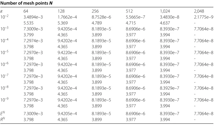
In this section, we verify experimentally the theoretical results obtained in the preceding section. The error estimates and convergence rates for the hybrid difference scheme are presented for two examples presented in [].
Example . Consider the reaction-diffusion problem
–εu(x) +u(x) =f(x), x∈–∪+, u() =u() =f(),
where
f(x) =
⎧ ⎨ ⎩
–.x, ≤x≤.,
., . <x≤.
The exact solution of this example is
u(x) =
⎧ ⎨ ⎩
.(ξ+η)(e–(.–x)/ε–e–(.+x)/ε) – .x, ≤x≤.,
.(ξ–η)e–/(ε)(e–(x–)/ε–e–(–x)/ε) + .( –e–(–x)/ε), . <x≤,
where the constantsξandηare
ξ=ε–e
–/(ε)
+e–/ε , η=. –e
–/(ε)
–e–/ε .
We measure the accuracy in the discrete maximum norm
eNε =max
≤i≤N|uε,i–Uε,i|, E N=max
ε e N ε,
and the ‘Shishkin’ convergence rate
rNε = lne N ε –lneεN
ln(lnN) –ln(ln(N)),
RN= lnE
N–lnEN
ln(lnN) –ln(ln(N)).
Numerical results for Example . are listed in Table .
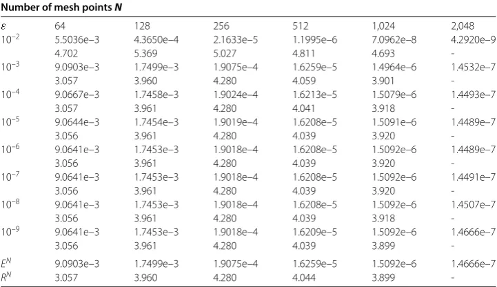
Example . Consider the reaction-diffusion problem
Table 1 Error estimates and convergence rates for variousNfor Example 5.1
Number of mesh pointsN
ε 64 128 256 512 1,024 2,048
10–2 3.4894e–3 1.7662e–4 8.7528e–6 5.5665e–7 3.4830e–8 2.1775e–9
5.535 5.369 4.789 4.715 4.637
-10–3 7.3009e–3 9.4205e–4 8.1893e–5 8.6906e–6 8.3930e–7 7.7064e–8
3.799 4.365 3.899 3.977 3.994
-10–4 7.2974e–3 9.4202e–4 8.1893e–5 8.6906e–6 8.3930e–7 7.7064e–8
3.798 4.365 3.899 3.977 3.994
-10–5 7.2970e–3 9.4220e–4 8.1893e–5 8.6906e–6 8.3930e–7 7.7064e–8
3.798 4.365 3.899 3.977 3.994
-10–6 7.2970e–3 9.4202e–4 8.1893e–5 8.6906e–6 8.3930e–7 7.7064e–8
3.798 4.365 3.899 3.977 3.994
-10–7 7.2970e–3 9.4202e–4 8.1893e–5 8.6906e–6 8.3930e–7 7.7064e–8
3.798 4.365 3.899 3.977 3.994
-10–8 7.2970e–3 9.4202e–4 8.1893e–5 8.6906e–6 8.3929e–7 7.7064e–8
3.798 4.365 3.899 3.977 3.994
-10–9 7.2970e–3 9.4202e–4 8.1893e–5 8.6906e–6 8.3930e–7 7.7064e–8
3.798 4.365 3.899 3.977 3.994
-EN 7.3009e–3 9.4205e–4 8.1893e–5 8.6906e–6 8.3930e–7 7.7064e–8
RN 3.798 4.365 3.899 3.977 3.994
-where
b(x) =
⎧ ⎨ ⎩
x+ , ≤x≤.,
( –x) + , . <x≤,
f(x) =
⎧ ⎨ ⎩
–., ≤x≤.,
., . <x≤.
The exact solution of this example is not available. Therefore, we use the double mesh principle to estimate the errors and compute the experiment convergence rates. Because mesh points forNand Ndo not match, we use the piecewise cubic spline interpolation to get the solution for N. That is,U¯N
ε (x) is a piecewise cubic spline interpolation of the
approximated solutionUN
ε , andU¯εN(xi) is the value of the functionU¯εN(x) at mesh point xiforN. We measure the accuracy in the discrete maximum norm
eNε =max
≤i≤N
UεN,i–U¯εN(xi), EN=maxε eNε,
and the ‘Shishkin’ convergence rate
rNε =
lneN ε –lneεN
ln(lnN) –ln(ln(N)),
RN= lnE
N–lnEN
ln(lnN) –ln(ln(N)).
Numerical results for Example . are listed in Table .
Table 2 Error estimates and convergence rates for variousNfor Example 5.2
Number of mesh pointsN
ε 64 128 256 512 1,024 2,048
10–2 5.5036e–3 4.3650e–4 2.1633e–5 1.1995e–6 7.0962e–8 4.2920e–9
4.702 5.369 5.027 4.811 4.693
-10–3 9.0903e–3 1.7499e–3 1.9075e–4 1.6259e–5 1.4964e–6 1.4532e–7
3.057 3.960 4.280 4.059 3.901
-10–4 9.0667e–3 1.7458e–3 1.9024e–4 1.6213e–5 1.5079e–6 1.4493e–7
3.057 3.961 4.280 4.041 3.918
-10–5 9.0644e–3 1.7454e–3 1.9019e–4 1.6208e–5 1.5091e–6 1.4489e–7
3.056 3.961 4.280 4.039 3.920
-10–6 9.0641e–3 1.7453e–3 1.9018e–4 1.6208e–5 1.5092e–6 1.4489e–7
3.056 3.961 4.280 4.039 3.920
-10–7 9.0641e–3 1.7453e–3 1.9018e–4 1.6208e–5 1.5092e–6 1.4491e–7
3.056 3.961 4.280 4.039 3.920
-10–8 9.0641e–3 1.7453e–3 1.9018e–4 1.6208e–5 1.5092e–6 1.4507e–7
3.056 3.961 4.280 4.039 3.918
-10–9 9.0641e–3 1.7453e–3 1.9018e–4 1.6209e–5 1.5092e–6 1.4666e–7
3.056 3.961 4.280 4.039 3.899
-EN 9.0903e–3 1.7499e–3 1.9075e–4 1.6259e–5 1.5092e–6 1.4666e–7
RN 3.057 3.960 4.280 4.044 3.899
-6 Conclusion
In this paper, we presented a high-order finite difference method for solving a singularly perturbed reaction-diffusion problem with a discontinuous source term. This difference scheme is a combination of a nonequidistant generalization of the Numerov scheme on the Shishkin-type mesh except for the point of discontinuity and a second-order differ-ence scheme on an additional refined mesh at the point of discontinuity. This hybrid dif-ference scheme for the singularly perturbed reaction-diffusion problem with a discon-tinuous source term is a modification of the difference scheme used in [–] for the singularly perturbed reaction-diffusion problem with sufficiently smooth data. Although the difference scheme does not satisfy the discrete maximum principle, the maximum norm stability of the scheme is established. We have shown that the scheme has accuracy O((N–lnN)) in the discrete maximum norm, independently of perturbation parameter.
Numerical experiments support these theoretical results.
Acknowledgements
We would like to thank the anonymous reviewer for some suggestions for the improvement of this paper. The work was supported by Humanities and Social Sciences Planning Fund of Ministry of Education of China (Grant No. 14YJC790006), Zhejiang Province Natural Science Foundation (Grant No. Y17D010024), Ningbo Municipal Natural Science Foundation (Grant Nos. 2017A610131, 2017A610140, 2015A610161), Ningbo Municipal Soft Science Foundation (Grant
No. 2015A10045) and Soft Science Project of Zhejiang Province (Grant No. 2015C35007).
Competing interests
The authors declare that there is no conflict of interests regarding the publication of this paper. The authors confirm that the mentioned received funding in the ‘Acknowledgements’ section does not lead to any conflict of interests regarding the publication of this manuscript.
Authors’ contributions
All authors read and approved the final manuscript.
Author details
1College of Finance and Trade, Ningbo Dahongying University, Ningbo, China.2Institute of Mathematics, Zhejiang Wanli
University, Ningbo, China.
Publisher’s Note
Received: 30 March 2017 Accepted: 7 July 2017
References
1. Chandru, M, Prabha, T, Shanthi, V: A hybrid difference scheme for a second-order singularly perturbed reaction-diffusion problem with non-smooth data. Int. J. Appl. Comput. Math.1, 87-100 (2015)
2. Miller, JJH, O’Riordan, E, Shishkin, GI, Wang, S: A parameter-uniform Schwarz method for a singularly perturbed reaction-diffusion problem with an interior layer. Appl. Numer. Math.35, 323-337 (2000)
3. Farrell, PA, Hegarty, AF, Miller, JJH, O’Riordan, E, Shishkin, GI: Robust Computational Techniques for Boundary Layers. Chapman & Hall/CRC Press, New York (2000)
4. Kadalbajoo, MK, Gupta, V: A brief survey on numerical methods for solving singularly perturbed problems. Appl. Math. Comput.217, 3641-3716 (2010)
5. Roos, H-G, Zarin, H: A second-order scheme for singularly perturbed differential equations with discontinuous source term. J. Numer. Math.10, 275-289 (2002)
6. Farrell, PA, O’Riordan, E, Shishkin, GI: A class of singularly perturbed semilinear differential equations with interior layers. Math. Comput.74, 1759-1776 (2005)
7. Boglaev, I, Pack, S: A uniformly convergent method for a singularly perturbed semilinear reaction-diffusion problem with discontinuous data. Appl. Math. Comput.182, 244-257 (2006)
8. de Falco, C, O’Riordan, E: Interior layers in a reaction-diffusion equation with a discontinuous diffusion coefficient. Int. J. Numer. Anal. Model.7, 444-461 (2010)
9. Rao, SCS, Chawla, S: Interior layers in coupled system of two singularly perturbed reaction-diffusion equations with discontinuous source term. Lect. Notes Comput. Sci.8236, 445-453 (2013)
10. Brayanov, IA: Numerical solution of a two-dimensional singularly perturbed reaction-diffusion problem with discontinuous coefficients. Appl. Math. Comput.182, 631-643 (2006)
11. Herceg, D: Uniform fourth order difference scheme for a singular perturbation problem. Numer. Math.56, 675-693 (1990)
12. Linß, T: Robust convergence of a compact fourth-order finite difference scheme for reaction-diffusion problems. Numer. Math.111, 239-249 (2008)
13. Sun, G, Stynes, M: An almost fourth order uniformly convergent difference scheme for a semilinear singularly perturbed reaction-diffusion problem. Numer. Math.70, 487-500 (1995)