A Reinforcement Learning Based Framework for Prediction of Near Likely Nodes in Data Centric Mobile Wireless Networks

(1)

Volume 2010, Article ID 319275,17pages doi:10.1155/2010/319275

Research Article

A Reinforcement Learning Based Framework for Prediction of

Near Likely Nodes in Data-Centric Mobile Wireless Networks

Yingying Chen,

1

_{Hui (Wendy) Wang,}

2

_{Xiuyuan Zheng,}

1

_{and Jie Yang}

1

1_{Department of Electrical Engineering, Stevens Institute of Technology, Hoboken, NJ 07030, USA}

2_{Department of Computer Science, Stevens Institute of Technology, Hoboken, NJ 07030, USA}

Correspondence should be addressed to Yingying Chen,[email protected]

Received 5 September 2009; Revised 8 May 2010; Accepted 10 June 2010

Academic Editor: Sayandev Mukherjee

Copyright © 2010 Yingying Chen et al. This is an open access article distributed under the Creative Commons Attribution License, which permits unrestricted use, distribution, and reproduction in any medium, provided the original work is properly cited.

Data-centric storage provides energy-eﬃcient data dissemination and organization for the increasing amount of wireless data.

One of the approaches in data-centric storage is that the nodes that collected data will transfer their data to other neighboring nodes that store the similar type of data. However, when the nodes are mobile, type-based data distribution alone cannot provide robust data storage and retrieval, since the nodes that store similar types may move far away and cannot be easily reachable in

the future. In order to minimize the communication overhead and achieve eﬃcient data retrieval in mobile environments, we

propose a reinforcement learning-based framework called PARIS, which utilizes past node trajectory information to predict the near likely nodes in the future as the best content distributee. Our framework can adaptively improve the prediction accuracy by

using the reinforcement learning technique. Our experiments demonstrate that our approach can eﬀectively and eﬃciently predict

the future neighborhood.

1. Introduction

The development of data-centric storage has enabled eﬃcient data dissemination of wireless networks. In data-centric storage, data is stored by attributes or types (e.g., geographic location and event type) at nodes within the network [1–

3]. Queries for data with a particular attribute will be sent directly to the relevant node(s) instead of performing flood-ing throughout the network, thereby data-centric storage enables eﬃcient data dissemination/access.

In data-centric storage of wireless networks, wireless devices that collect the data are called collector nodes. Whereas the data can be stored on other nodes, called

storage nodes [3–5], based on their attributes or types. Most existing data-centric storage models can only deal with staticwireless networks. However, with the increasing deployment of wireless devices, there are emerging pervasive applications that rely on the mobility of wireless device. Two representative examples are: (1) sensors are used for animal migration tracking, and (2) wireless devices are equipped with police oﬃcers to monitor their daily patrol routes, collect crime information by areas, and record corresponding

law enforcement actions. In these two scenarios, eﬃcient data retrieval can be achieved if the data-centric storage is enabled, that is, the data is stored by the types of animals, by the activities performed by the animals, or by the tasks that are carried out by the police oﬃcers. The challenge is to design schemes that can support data-centric storage when all the nodes are moving around. In this paper, we consider a fully distributed network, in which there is no node playing the sole role as storage; each node can act as both the collector and storage node. For instance, a wireless node, playing the role of a collector node, can collect data of more than one type, but usually it only stores one type of data and transfers the rest of data of other data types to other nodes, which are the storage nodes corresponding to this collector node. Further, to reduce the communication overhead, the storage nodes are picked from the neighborhood, that is, the nodes in the transmission range, of the collector node.

(2)

future. Thus, when a user sends queries to the collector nodes, the queries need to be redirected to those storage nodes with much communication overhead. Therefore, it is desirable that the collector nodes migrate their data to the storage nodes that not only possess similar data types but also highly likely to travel with them in the future. We define this kind of storage nodes as near likely nodes, which are the nodes that are in the neighborhood (i.e.,

near) and carry the same type of data that needs to be stored (i.e., likely). In this paper, we propose mechanisms to predict near likely nodes for data-centric mobile wireless networks to achieve eﬃcient data storage and retrieval. More specifically, we proposePARIS, a fully distributed neighbor-hood prediction framework based on reinforcement learning techniques that utilize past node trajectory information to determine the best content distributee for the future. We first define a probability-based neighborhood prediction model. We then propose two approaches, namely point-based and

traced-based, that predict the future neighborhood based on the correlations of the past trajectories. Moreover, we develop WINTER (WINdow adjusTment with Expanding and shRinking) algorithm, which can perform adaptive adjustment during runtime and improve the prediction accuracy by using the reinforcement learning technique. In addition, a probability-based metric is developed to measure the accuracy of prediction. Our approach of data transfer based on neighbor prediction helps to reduce com-munication overhead and consequently the overall energy consumption during data retrieval because the storage nodes most likely move together.

To evaluate the effectiveness and efficiency of our scheme, we conducted experiments using mobile wireless networks simulated based on a city environment and its vicinity in Germany [6, 7]. By examining two representative scenar-ios, walking scenario, and vehicular driving scenario, our experimental results show high-prediction accuracy and low-computational time when using PARIS, thereby providing strong evidence of the effectiveness of using data-centric approach through the prediction of near likely nodes in mobile wireless applications.

The rest of the paper is organized as follows. We place our work in the context of the related research inSection 2. In Section 3, we provide an overview of our problem and formulate our probability-based neighborhood prediction model. We next discuss the likelihood of neighborhood by presenting our two prediction approaches and the new metric for measuring accuracy prediction in Section 4. Further, we present the protocols of data transfer and data retrieval and our adaptive accuracy adjustment using reinforcement learning under the PARIS framework in

Section 5. We present the experimental evaluation of our approach in Section 6. Finally, we conclude our work in

Section 7.

2. Related Work

There has been active work on data-centric storage in sensor networks. In addition to the approaches of global data storage in which the wireless device data is aggregated to be

stored at external central servers, algorithms of local infor-mation processing [8], and wide-area data dissemination [9, 10] are proposed.Reference [8] used signal processing techniques to collaborate among local nodes for information processing. References [9,10] proposed directed diﬀusion algorithms that implement in-network aggregation and allow nodes to access data by name across wireless networks. Further, recent work is more focused on data-centric storage [1–3,5], where the data is stored decentralized by attributes and types.Reference [1] achieved data-centric storage based on the GPSR routing algorithm and an eﬃcient peer-to-peer lookup system.Reference [2] developed schemes for resilient data-centric storage from the viewpoint of energy savings and scalability in wireless networks. Whereas the security and privacy concerns in data-centric storage are addressed in [3]. Most of these current works only deal with static

sensor networks. In this paper, we study data-centric storage inmobilewireless networks.

To detect mobility of wireless nodes, [11] used received signal strength in wireless LAN to detect wireless device mobility.Reference [12] determined mobility from GSM traces using diﬀerent metrics. In [13] signal variance is used with Hidden Markov Model (HMM) to eliminate oscillations between the static and mobile states for mobility detection. Further, [14] proposed to use correlation coeﬃcients on RSSI traces to detect wireless devices that are moving together.

The works that are most closely related to ours are [15–17]. A user-centric approach was proposed in [15] for colocation prediction that is used for media sharing based on repeating similar journeys in the urban transportation environment. Unlike [15], our approach does not require repeated trajectory patterns, and thus is more generic and can be applied to a broad array of pervasive applications involving mobile devices. References [16,17] addressed the detection of nodes of similar mobility patterns in group caching in MANET. However, these works do not support fully distributed models. Further, their work focused on

current neighbors, not the prediction of future ones. Our work is novel in that we utilize the past node trajectories to predict the future co-movement of nodes for data-centric storage in mobile environments.

3. Problem Overview

In this section, we first present our assumptions. We then provide an overview of PARIS and define our probability model for neighborhood prediction.

3.1. Assumptions. When considering data-centric mobile wireless networks, we have the following assumptions.

(i)Mobility. Wireless device are moving, randomly or in some pattern, in a well-defined area, though the nodes are not aware of their moving patterns, if there is any. There are no predefined trajectories for each node. However, we assume that there exists a

(3)

may travel to visit the Metropolitan Museum together and they use their mobile phones to take pictures, shoot videos, and write multimedia blogs on the way.

(ii)Location-Aware. We assume that the nodes know their physical locations at all time points during moving. It is a reasonable assumption because in many cases the data is useful only if the location of its source is known. For example, knowing that a crime occurred, which requires a law enforcement action, but without knowing where it occurred is useless. Localization of the mobile nodes can be achieved through the use of GPS or some other approximates but less burdensome localization algorithms [18,19].

(iii)Neighborhood.Each node has a short communication range and can communicate only with nodes within its transmission range. We call the nodes in the transmission range theneighbors. Mobility of wireless devices may result in the change of the neighbor-hood. However, we assume that for every node, it has a stable neighborhood within a period of time. For example, police oﬃcers who carry out the same tasks are kept in neighborhood while they are on duty.

(iv)Data-centric storage. We assume that the storage is

data-centric, that is, the particular node that stores a given data object is determined by the object’s type such as event type [1,2]. Hence, all data with the same type will be stored at the same node (not necessarily the collector node), so that the subsequent data retrieval requests could be eﬃciently directed. In particular, we propose to transfer data of the same type to a node’s near likely nodes. The subsequent data queries will reach a collector node first through routing protocols for mobile wireless networks [20] and will then be redirected to the corresponding storage nodes.

3.2. Overview of PARIS. Data-centric approaches provide low-communication overhead and efficient search, however applying data-centric mechanisms to mobile environments brings new challenges. Since mobility of nodes can change the reachability of nodes and consequently affect the rout-ing decision and long-term storage capability, data-centric storage in mobile wireless networks must take mobility into consideration. In mobile wireless networks, when a node stores its data on other nodes [1,2], it is desirable that the chosen nodes are in the neighborhood in the future, so that when there come the requests for the data, the collector node can efficiently redirect the requests to its near likely nodes that store the data in its neighborhood.

In PARIS, we study how to store and retrieve data eﬃciently by making use of neighborhood predication for data-centric storage in mobile wireless networks. In addition, PARIS can be easily extended to help in load balancing when a node exceeds its storage. The main logical components in PARIS are on-demand data transfer, runtime update of near likely node (for eﬃcient data retrieval), and adaptive

adjustment through reinforcement learning. By on-demand data transfer, each collector node calculates its near likely node only when it needs to transfer its data to another node. During data retrieval, the collector node is responsible to redirect the corresponding queries to its near likely node. If at a later time, the near likely node that carries the data from a collector node is moving out of the neighborhood of the collector node, the collector node will run the neighborhood prediction process again and perform a runtime update to transfer the data from the storage node to its current near likely node. As it is only performed at certain time points, the on-demand data transfer mechanism reduces both the communication overhead and energy consumption in the neighborhood prediction procedure. Additionally, the WINTER algorithm based on the reinforcement learning technique is developed to adaptively improve the accuracy of neighborhood prediction in each prediction round. The details of PARIS will be presented inSection 5.

3.3. Probability Model. Generally, with mobile devices, the neighborhood may change over time. Some nodes may move into or move out of the transmission range periodically. To predict the future neighborhood, we utilize thetrajectoryof the mobile devices. We assume the position of the nodes at each time point is in a 2-dimensional space. We note that our results can be easily extended to more than two dimensions. We denote the location of mobile node s at time t as st(x,y), where x and y denote the x- and y

-coordinates ofsat time pointt. Then given a time window

W(t1,. . .,tm) that consists ofmtime points, the trajectory

of nodesofWis denoted asT(st1(x,y),. . .,stm(x,y)). Given

a set of trajectories T{T1,. . .,Tn}of n nodes, our goal is

to useT to predict the neighborhood ofsat a future time pointti > tm. To achieve this goal, we define a probability

model of prediction that quantifies the likelihood of the future neighborhood. Since we assume that for every node, it has a stable neighborhood within a period of time, our prediction is based on the principle thatthe nodes that are not only the neighbors in the past but also moving in the same direction are highly likely to be neighbors in the near future. Based on this, we define two probability parameters.

(1)Neighborprobability Prn: it is used to reflect the belief

from the trajectoriesT that a nodesis in the same neighborhood of the nodes.

(2)Direction probability Prd: it is used to measure the

likelihood from the trajectoriesT that two nodess

andsare moving in the same direction.

We further define the belief probability that nodesis in the neighborhood ofsin the future as Prdtexpressed by

Prdt=Prn∗Prd. (1)

Given the time window W, a collector node s and its neighbor nodes, if s needs to store its data on its near likely node, then from its neighbor nodes that have available storage and store the same type of data that needs to be transferred froms,spicks the node that is of the maximum Prdt. Our model can be easily extended to choosek nodes

(4)

1.05

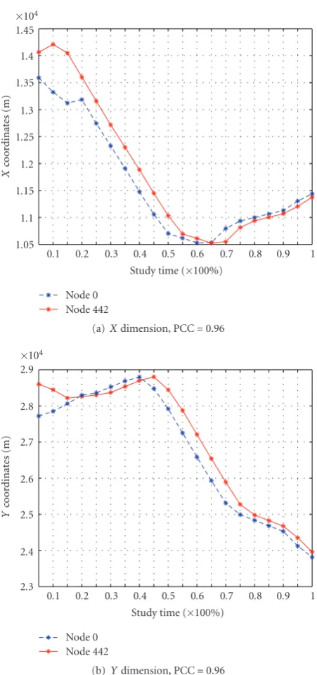
Figure1: Illustration of thexandycoordinates versus time series for nodes 0 and 442 when they are moving together.

4. Neighborhood Likelihood

In this section, we first explain how to compute the neighbor probability Prn. We then propose two approaches, namely,

trace-basedandpoint-based, to calculate the direction prob-ability Prd. We next develop a new metric that measures the

prediction accuracy.

4.1. Neighbor Probability. Given a node s within a time windowW(t1,. . .,tm), for any nodes, letN(s)={ti |1 ≤

Intuitively at more time points thatsis in the neighborhood ofsin the past, it will be more likely thats remains as the neighbor ofsin the future.

4.2. Direction Probability. If two nodes are moving in the same direction, they should have similar trajectories and theirx- andy-coordinates must follow the similar traces, and consequently may result in a strong correlation between their x- and y-coordinates, respectively, and vice versa. Figure 1

shows an example of the coordinates versus time series when two nodes move together. We observed that the two nodes have highly-correlated traces in bothXandYdimensions.

Thus, to measure whether two nodes are moving in the same direction, we use thePearson correlation coeﬃcient[21]. In general, the Pearson correlation coeﬃcient is a statistical method that measures the strength and direction of a linear relationship between two given random variables. More specifically, given two random variablesP= {p1,. . .,pn}and

standard deviation ofP andQ. The PCC value ranges from

−1 to +1. Correlation +1/−1 means that there is a perfect positive/negative linear relationship between P and Q. In

Figure 1, the high PCC value 0.96 for both theXdimension and the Y dimension shows high correlation between the coordinates of two nodes that are moving together.

Further, to measure the direction probability, we develop two schemes, point-based and trace-based, based on the Pearson correlation coeﬃcient. These two schemes consider both spatial and temporal changes of nodes in mobile environments.

4.2.1. Point-Based Scheme. This approach utilizes the mov-ing direction of the nodesandsat each time pointtiwithin a

time windowWto determine whether two nodes are moving together. The key idea is that the collector node computes the moving directions of the neighbor nodes at all time points in the time windowW and measures the Pearson correlation coeﬃcients of the moving directions.

Given the node s and its trajectory T(st1(x,y),. . ., stm(x,y)), wheresti·xandsti·yare thexandycoordinates

of the node at each time pointti(1< i≤m) respectively, we

define thegradientθito measure the moving direction at the

time pointti

θi=sti·y−sti−1·y

sti·x−sti−1·x

. (4)

(5)

t1 t2 t2 t3 t4 X Y

Figure2: An example of direction measurement.

example. Although the gradientθmay not be accurate when the trajectory between the time pointsti−1andtiis not linear,

we argue that we can always reduce the error by adding more time points on the nonlinear trajectories, so that the subtrajectories are close to linear format. For example, as shown in Figure 2we can split the non-linear trajectories betweent2andt3into smaller units by adding a time pointt2

betweent2andt3, as a result the trajectories betweent2and

t2as well as betweent2andt3are close to linear.

Finally, we measure the Pearson correlation coeﬃcient ofΘ1

andΘ2. If the coeﬃcient is positive, we take it as the direction

4.2.2. Trace-Based Scheme. In this approach, opposite to the point-based approach, the collector node does not calculate the moving direction at each time point. Instead, it measures the Pearson correlation coeﬃcients of two trajectories. To be more specific, given two trajectories T and T of two nodes s and s, first, the collector node s computes the Pearson correlation coeﬃcient between thex-coordinates of

T and that of T and collects the positive coeﬃcients cx.

Similarly, it calculates the Pearson correlation coeﬃcient of they-coordinates ofTand that ofT. Let the set of positive

As illustrated in Figure 1, when two nodes are moving together, the values of correlation coeﬃcients are high in

bothXandYdimensions. Since the correlation coeﬃcients onXandYdimensions are independent, we multiplycxand

cyas the direction probability

Prd=cx∗cy. (7)

Moreover,Prdis normalized as needed.

4.3. Measurement of Accuracy of Neighborhood Prediction.

One challenge of data-centric mobile wireless networks is the eﬃciency of data retrieval, which highly depends on the accuracy of neighborhood prediction results. Wrong prediction results may cause data to be stored on unreachable nodes and thus incur expensive communication overhead and consume more energy. Therefore, it is necessary to measure the accuracy of neighborhood prediction and evaluate the eﬀectiveness of our prediction schemes. In this section, we present our new metric Prediction Accuracyin measuring neighborhood prediction accuracy.

In Prediction Accuracy metric, the time points are split into two time windows, pastWpand futureWf. The window

of pastWp is used as the “training set” to predict the near

likely nodes, whereas the window of futureWf, is used as the

“test set” to verify the accuracy of the prediction. We choosen

nodes, denoted asS, as the “test participants”. Our accuracy measurement consists of two steps.

Step 1(Training). For each node si(1 ≤ i ≤ n) in S, we

find its near likely nodesithat is of the maximum Prdtin the

time windowWp. Fornnodes, we collectnsuch neighbor

nodes and put their Prdtinto a vectorP. ThusPconsists ofn

probability values.

Step 2(Testing). For each near likely neighborsi (1≤i≤n)

fromStep 1, we calculate its Prdtof the windowWf and store

Prdtin a vectorQ, which is also a set ofnprobability values.

Our measurement of accuracy is based on the distance ofP

andQ. The smaller the distance is, the more accurate the prediction result will be.

To measure the distance of two probability distribution

P and Q, our metric of Prediction Accuracy is based on KL-divergence. KL-divergence is a noncommutative measure of the diﬀerence between two probability distributions in probability theory and information theory [22]. Specifically, for probability distributionsP andQ, the KL-divergence of

QfromPis defined as

DKL(Q,P)=

i

QilogQi

Pi. (8)

The smaller the value ofDKL is, the moreQis similar toP, which consequently indicates that our prediction of future near likely node is more accurate.

(6)

shows that the neighborhood of these nodes is changing in the future window. Since KL-divergence only shows the

aggregate result of the diﬀerence of two probabilities, to study the prediction error at a more detailed level, we use

Cumulative Distribution Function (CDF). Specifically, given the probability distributions P from the past window and

Q from the future window, we compute the positive and

negativeprobability diﬀerence vectors PD+and PD−:

PD+= {Q[i]−P[i]|Q[i]−P[i]≥0},

PD−= {Q[i]−P[i]|Q[i]−P[i]<0}.

(9)

The nodes in PD+(PD−, resp.) are the ones whose

probabil-ities are increasing (decreasing, resp.). We measure CDF of both PD+ and PD−. Intuitively, the closer the distributions

of PD+ and PD− to the value 0 are, the more accurate the

prediction is.

5. Framework of PARIS for Data Transfer and

Data Retrieval

In this section, we describe the three main logical compo-nents in PARIS framework, on-demand data transfer, run-time update of near likely nodes, and adaptive adjustment through reinforcement learning.

5.1. On-Demand Data Transfer. In PARIS, data transfer happens on-demand, that is, when a collector nodesneeds to transfer its data to other nodes, and the communication between nodes is only performed at the specific time point. Thus, the on-demand scheme reduces the communication overhead and energy consumption incurred from frequent information exchange. There are two requirements when choosing the nodes that the data will be transferred to

(i) Following the data-centric requirement, the collector node picks the neighbor nodes that have not only suﬃcient storage but also the matching type of data that will be transferred.

(ii) If there are multiple nodes that satisfy the first requirement, the collector node will pick the node with the largest Prdt.

The on-demand data transfer procedure consists of three steps.

(1) A collector nodessends a request to all the nodes in its neighborhood. The request consists of the inquiry of the allowed data type, the size of the available storage, and the trajectory of the nextmtime points in the time windowW. The neighbor nodes reply the request ofswith proper information.

(2) The collector node scollects the answers and picks the node that satisfies the above two requirements as the near likely nodes.

(3) The collector node s sends its data to its near likely nodes, and updates itsdata tracktable. The data track table consists of entries in the format of

(IDXd, IDs), with each entry used for tracking which

node the data is stored on, so that when there is a user query for the data, nodescan eﬃciently redirect the query. The IDs is the node identity of the near

likely node that stores data with index IDXd in the

data track table.

5.2. Runtime Update of Near Likely Node. Given the fact that the estimated near likely node has a belief probability to be in the neighborhood in the future, it is possible that when a data query arrives at a future time point, the near likely node has already moved out of the neighborhood of the collector node. This will increase the communication overhead in order to locate the “previous” near likely node for data retrieval. In order to minimize the communication overhead, it is desirable to always keep the transferred data in the neighborhood of the collector node in a mobile wireless network environment.

We propose runtime update of the near likely node in PARIS. Usually in wireless networks each node keeps a list of its neighbors and update the list periodically based on the communication of beacon packets [23]. Upon each neighbor update, the node checks its data track table. If a node identity, which appears in the data track table, has disappeared from its neighbor list, the node needs to perform a runtime update to find its current near likely node. To avoid frequent runtime updates and consequently much update overhead, it is desirable to look for the current near likely node of the same data type as the replacement. The following steps will take place:

(1) The collector nodesruns step 1 and 2 from the on-demand data transfer procedure for the correspond-ing type of data with IDXdand identifies a new near

likely nodes.

(2) The collector node s then sends a request to the previous near likely nodesand askssto transfer the data with IDXdto nodes.

(3) Once the collector nodesreceives the confirmation fromsthat the data transfer is successful, it updates its data track table by replacing (IDXd,IDs) with

(IDXd, IDs).

A node may be identified as a near likely node for more than one collector nodes. In PARIS, the near likely node is stateless, whereas the collector nodes keep a data track table to maintain the data transfer information. The advantage of the runtime update of near likely node is that the data is stored on either the collector node itself or its near likely nodes. Thereby no flooding messages are needed during data retrieval, and thus reduce the overall communication overhead.

(7)

(1) Letsands_{be the collector node and its predicted near likely neighbor;}

(2)i←0;

(3)repeat

(4) LetKL1andKL2be the KL-divergence measured from time windowWiandWi+1;

(5) Letoptbe the operation (expansion or shrinkage) on time windowWi+2;

(6) if(KL2< KL1)then

(7) //KL-divergence improves;

(8) ifopt==“expansion”then

(9) The size of the next time window|Wi+2| = |Wi+1|+ 1;{Expansion;}

(10) else

(11) The size of the next time window|Wi+2| = |Wi+1| −1;−1;{Shrinkage;}

(12) end if

(13) else

(14) //KL-divergence falls;

(15) ifopt==“expansion”then

(16) The size of the next time window|Wi+2| = |Wi+1| −1;

(17) opt←“shrinkage”;{Shrinkage;}

(18) else

(19) The size of the next time window|Wi+2| = |Wi+1|+ 1;

(20) opt←“expansion”;{Expansion;}

(21) end if

(22) end if

(23) i←i+ 1;

(24)untilThe time points are exhausted;

Algorithm1: The WINTER algorithm.

expensive energy consumption and increased communica-tion overhead if the update is frequent. The reason for such frequent update is the prediction of near likely neighbors that is not accurate enough. As shown in Section 4.3, the prediction accuracy is aﬀected by the configuration of time windows that are used to collect the past trajectories of a node. Time windows that are too small cannot capture the correct neighborhood and cause inaccurate neighbor prediction, while time windows that are too large will consume more energy on each neighboring nodes for collecting trajectory traces and increase the communication overhead when sending the trajectory traces to the collector node. Therefore, the appropriate time window will allow PARIS to be eﬀective for neighborhood prediction.

To improve the neighbor prediction accuracy, we adap-tively adjust the time windows by applying thereinforcement learning mechanism from the beginning of the whole procedure. Reinforcement learning is a machine learning technique that deals with sequential control problems [24].

Our goal is that according to the current state, that is, the current neighborhood prediction, determines how to revise the size of the time window to reach a better neighborhood prediction in the next round. The revision of the time windows consists of two operations:expanding, that is, increasing the window size by one time point, and

shrinking, that is, decreasing the window size by one time point. The collector node s keeps an observation of the change of KL-divergence incurred by expansion/shrinkage of the time window. We say the prediction accuracyfallsif the KL-divergence increases. Otherwise, we say the prediction accuracyimproves. Based on this, we developed an algorithm

based on reinforcement learning, called WINTER (WINdow adjusTment with Expanding and shRinking), which adap-tively adjusts the time window size by the following:

(i) If the prediction accuracyfallsfrom time windowWi

to Wi+1, then for time window Wi+2, we “reverse”

the operation, that is, if the operation on Wi+1 is

expansion/shrinkage, we shrink/expand forWi+2.

(ii) Otherwise, the prediction accuracy improves from time windowWitoWi+1. Then we repeat the same

operation onWi+1forWi+2.

After a sequence of expansions and shrinkages, it is possible that diﬀerent collector nodes have time windows of diﬀerent sizes.

The pseudocode that implements WINTER is shown in

Algorithm 1.

6. Experimental Evaluation

In this section, we describe our experimental methodology and present the results that evaluate the eﬀectiveness of our approaches.

(8)

Figure3: The experimental data sets are generated based on the city and its vicinity in Germany.

scenarios, one is in walking speed of 4 ft/s, and the other is in vehicular driving speed of 50 ft/s. For the walking scenario, two data sets, we callsmallandlarge, are obtained using this simulation environment with 1000 and 5000 nodes generated, respectively, and placed randomly inside the city.

For the vehicular driving scenario, one data set is created through the simulation environment with 1000 nodes gener-ated and placed randomly inside the city. For the duration of our study, some new nodes may move into the city environment and some existing nodes may move out the city environment. There are no pre-defined trajectories for each node. However, group of nodes may travel together to common destinations (e.g., the city center).Figure 4presents the average number of neighbors when using the small data set in walking scenario for the duration of our study time, shown as percentage from 0 to 1, for 600 nodes and 100 nodes, respectively.

The 100 nodes are randomly chosen from 600 nodes. We observed that the average number of neighbors increases from a few nodes to around 14 nodes as the study time moves along, indicating that groups of nodes are gradually formed and traveling together to the similar destinations. The vehicular driving scenario has the similar trend as the walking scenario. This is in line with our co-movement assumption. Thus, these datasets are suitable for our neigh-borhood prediction study.

6.2. Metrics. We will utilize the following performance metrics to evaluate the eﬀectiveness of PARIS in terms of prediction of near likely nodes.

Prediction Accuracy. As described inSection 4.3, the Predic-tion Accuracy metric measures the statistical characteristics of neighborhood prediction based on the Cumulative Dis-tribution Function (CDF) of the diﬀerence of the future probability Prdtto the past probability Prdtof the near likely

node on top of the KL-divergence. We split our study time to a past time window for prediction and a future time window to evaluate our prediction. In the following discussion, we use the percentage of study time as the measurement of window size.

We investigate the impact of diﬀerent window sizes of the past as well as the future on the prediction accuracy using both point-based and trace-based schemes.

(9)

7

Figure4: Average number of neighbors versus study time when using the small data set.

6.3. Results

KL-Divergence. We first study the neighborhood prediction accuracy in our proposed mechanism for both walking and vehicular speed scenarios. Figure 5 presents values of KL-divergence versus diﬀerent past window sizes when fixing the future window size, whereasFigure 6presents values of KL-divergence versus diﬀerent future window sizes when fixing the past window size for both point-based as well as trace-based schemes under the case when the average number of neighbors is 5.

For the walking speed scenario, we observed small KL-divergence values that are always less than 0.5. This is encouraging as the smaller KL-divergence values indicate that the distribution of the belief probability in the future is close to the distribution of that in the past. Further, as shown in Figures 5(a) and5(b), when fixing the time window of the future, 0.2 and 0.4 of the total study time, respectively, as the size of the past time window increases, the KL-divergence value presents an overall decreasing trend

for the point-based scheme. This means that by using the point-based scheme, the larger the past window size, the more accurate the prediction of near likely node can become. However, for the trace-based scheme, we observed that the KL-divergence value fluctuates. This is interesting since it shows that for the trace-based scheme, simply increasing the past window size does not increase the accuracy, which indicates that we need both expansion and shrinkage for adaptive adjustment of window sizes.

On the other hand, when fixing the time window of the past, 0.2 and 0.4 of the total study time, respectively, as presented in Figures6(a)and6(b), we observed an increasing trend of the KL-divergence value for both schemes as the window size of future is increasing when the average number of neighbors is 5, indicating that the near likely node may gradually move away from the collector node when the future is long enough.

We also investigate the neighbor prediction accuracy in our proposed mechanism for the vehicular driving scenario. Figures5(c) and6(c) present the neighborhood prediction accuracy in the vehicular-driving scenario. First, similar to the walking scenario, the values of KL-divergence are less than 0.5, which indicates that our scheme obtains accurate prediction accuracy in the vehicular driving scenario as in the walking scenario. We also observed similar changing trend as the result of walking scenario.

In particular, as shown in Figure 5(c), when fixing the future window size to 0.4 of the total study time, as the size of the past window size increases, the KL-divergence value presents an overall decreasing trend, which is similar to the trend inFigure 5(b). While fixing the past window size to 0.4 as shown inFigure 6(c), we also observed similar increasing trend and KL-divergence value as in Figure 6(b). Further, the increased amount of the KL-divergence values is always small (around 0.05). These results indicate that our proposed schemes are appropriate for diﬀerent mobility scenarios.

In general, we found that the KL-divergence values of trace-based scheme is smaller than those using point-based scheme for both walking and vehicular driving scenarios. Moreover, for the walking scenario, we observed similar results when the average number of neighbors increases to 15 and 45. Due to space limitation, the results are omitted. Therefore, the trace-based scheme has better prediction accuracy than the point-based scheme.

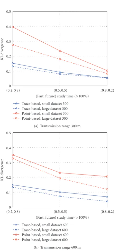
Further, we compared the values of KL-divergence between the small and the large data sets inFigure 7. In order to compare these two diﬀerent data sets directly, we used the same transmission range of the nodes in each data set, which is under 300 m and 600 m, respectively.

(10)

0 0.05 0.1 0.15 0.2 0.25 0.3 0.35 0.4 0.45 0.5

0.2 0.28 0.36 0.44 0.52 0.6 0.68 0.76 (Past) study time (×100%)

KL

di

ve

rgenc

e

Trace-based Point-based

(a) Walking Scenario: Future window 0.2

0 0.05 0.1 0.15 0.2 0.25 0.3 0.35 0.4 0.45 0.5

0.2 0.24 0.28 0.32 0.36 0.4 0.44 0.48 0.52 0.56 (Past) study time (×100%)

KL

di

ve

rgenc

e

(b) Walking Scenario: Future window 0.4

0 0.05 0.1 0.15 0.2 0.25 0.3 0.35 0.4 0.45 0.5

0.2 0.24 0.28 0.32 0.4 0.44 0.48 0.52 0.56 (Past) study time (×100%)

KL

di

ve

rgenc

e

(c) Vehicular Scenario: Future window 0.4

Figure5: KL-divergence: fixed future window size; (a) and (b) the future window size is set to 0.2 and 0.4 of the total study time, respectively, when the average number of neighbors is 5; (c) the future window size is set to 0.4 of the total study time when the average number of neighbors is 15.

Cumulative Distribution Function (CDF). Turning to study-ing the CDF of the diﬀerence of the future probability Prdt

to the past probability Prdtof the near likely node.Figure 8

presents the CDF of the probability difference for both point-based and trace-point-based schemes when the window size of the future is fixed as 0.2 of the total study time, whereas the window size of the past changes from 0.2 to 0.4 of the total study time. We found that for both the positive difference PD+ and the negative difference PD−, the CDF curve of the

trace-based scheme lies to the left side of the point-based scheme.

This shows that in terms of neighborhood prediction accuracy, the trace-based scheme outperforms the point-based scheme, which is inline with the results obtained from the KL-divergence.

Moreover, we investigated the prediction accuracy under the cases of diﬀerent average number of neighbors, that is, 5, 15, and 45, respectively, in the neighborhood. Figure 9

presents the CDF of PD+ for both of our schemes. We

(11)

0 0.05 0.1 0.15 0.2 0.25 0.3 0.35 0.4 0.45 0.5

0.2 0.28 0.36 0.44 0.52 0.6 0.68 (Future) study time (×100%)

KL

di

ve

rgenc

e

(a) Walking Scenario: Past window 0.2

0 0.05 0.1 0.15 0.2 0.25 0.3 0.35 0.4 0.45 0.5

0.2 0.24 0.28 0.32 0.36 0.4 0.44 0.48 0.52 0.56 (Future) study time (×100%)

KL

di

ve

rgenc

e

(b) Walking Scenario: Past window 0.4

0 0.05 0.1 0.15 0.2 0.25 0.3 0.35 0.4 0.45 0.5

0.2 0.24 0.32 0.36 0.4 0.44 0.48 0.52 0.56 (Future) study time (×100%)

KL

di

ve

rgenc

e

(c) Vehicular Scenario: Past window 0.4

Figure6: KL-divergence: fixed past window size; (a) and (b) the past window size is set to 0.2 and 0.4 of the total study time, respectively, when the average number of neighbors is 5; (c) the past window size is set to 0.4 of the total study time when the average number of neighbors is 15.

diﬀerent average number of neighbors. These results are very encouraging as it indicates that given a prediction scheme the prediction accuracy only relies on the window size.

Reinforcement Learning. We next examine the eﬀects of rein-forcement learning on prediction accuracy using WINTER algorithm.Figure 10presents the expansion/shrinkage of the prediction window (i.e., the past window) according to the obtained KL-divergence value. InFigure 10(a), we observed that when fixing the future testing window to 0.12, the pre-diction window size is adjusted adaptively based on the KL-divergence values; when the KL-KL-divergence value decreases from 0.043 to 0.02, the size of the prediction window expands

from 0.12 to 0.2, while the prediction window shrinks from 0.2 to 0.08 when the KL-divergence value increases from 0.02 to 0.039. We observed the similar window adjustment behavior inFigure 10(b). Further, we found that by adaptive adjustment, the KL-divergence values are always less than 0.05 (even less than 0.016 inFigure 10(b)). These results are encouraging as it indicates that our approach of adaptive adjustment through reinforcement learning is eﬀective in improving prediction accuracy during runtime.

(12)

0 0.1 0.2 0.3 0.4 0.5

(0.2, 0.8) (0.5, 0.5) (0.8, 0.2)

(Past, future) study time (×100%)

KL

di

ve

rgenc

e

Trace-based, small dataset 300 Trace-based, large dataset 300 Point-based, small dataset 300 Point-based, large dataset 300

(a) Transmission range 300 m

0 0.1 0.2 0.3 0.4 0.5

(0.2, 0.8) (0.5, 0.5) (0.8, 0.2)

(Past, future) study time (×100%)

KL

di

ve

rgenc

e

Trace-based, small dataset 600 Trace-based, large dataset 600 Point-based, small dataset 600 Point-based, large dataset 600

(b) Transmission range 600 m

Figure7: Comparison of KL-divergence between the small and the large data sets in walking scenario.

are always less than 0.05. This proves the eﬀectiveness of our adaptive adjustment approach. Second, we observed that although the study time in both Figures 11(a) and 11(b)

is scaled from 0 to 1, the similar window size adjustment behavior presents as with shorter study time (Figure 10). For example, in Figure 11(a), when fixing the size of the future testing window as 0.12, when the KL-divergence value increases from 0.02 to 0.038, the size of the prediction window shrinks from 0.12 to 0.08, while the prediction window expands from 0.08 to 0.16 when the KL-divergence

value decreases from 0.038 to 0.022. This demonstrates that our adaptive adjustment approach through reinforcement learning works in larger time windows as well.

Time Performance. Figure 12 presents the comparison of time measurements under various setups including diﬀerent average number of neighbors and various window sizes for both small and large data sets. We found that the time to perform neighborhood prediction is in the order of milliseconds for both schemes.

We observed that the point-based scheme runs at about two times faster than the trace-based scheme constantly under diﬀerent average number of neighbors and various window sizes. This is because the trace-based scheme needs to calculate correlation coeﬃcients for both X and Y

dimensions, whereas the point-based scheme only calculates the correlation coeﬃcient for gradient. Further, the time measurements of the large data set are also in the order of milliseconds as shown in Figure 12(b). This indicates that even when a node has large number of neighbors, our schemes can eﬃciently predict the near likely nodes.

Communication Overhead. Next, we measure the commu-nication overhead incurred by collecting the trajectory information from a collector’s neighbors. Let us consider the transmission packets of 512 bytes [25]. We assume that each trajectory record consists of a pair of (x,y) coordinates and a timestamp, each of float type. In other words, each trajectory record consists of 12 bytes. Therefore, one transmission packet can contain at most 42 trajectories. If one node records its trajectory every Y seconds, then the trajectory information ofXseconds can be stored inX/42Ypackets.

Moreover, we assume that for every F seconds, to apply the neighborhood prediction mechanism, the collector node needs to collect the trajectory of X seconds from its N neighbors. Therefore, there are X/42YFN packets transmitted to the collector node from its neighbors. Assume the collector node needs to transfer its data of size Z to the storage node within these F seconds. Then the size of the transmission packets needed for collecting trajectory information is X/42Y(N/Z) of the data sent to the identified near likely node by the collector node. We assume thatX/42Y(N/Z) is less than 1.

Based on our analysis, we can see that both the packet sizeX/42YFN and the percentage of transmission packets

X/42Y(N/Z) are not aﬀected by the moving speed of the mobile nodes. Thus, the communication overhead incurred from the trajectory information exchange in our approach is not sensitive to the mobility model.

(13)

0 0.1 0.2 0.3 0.4 0.5 0.6 0.7 0.8 0.9 1

0 0.2 0.4 0.6 0.8 1

Diﬀerence of future probability and current probability

P

robabilit

y

Point-based (0.2, 0.2), average number of neighbors 15 Trace-based (0.2, 0.2), average number of neighbors 15

(a) Positive diﬀerence (0.2, 0.2)

0 0.1 0.2 0.3 0.4 0.5 0.6 0.7 0.8 0.9 1

0 0.2 0.4 0.6 0.8 1

P

robabilit

y

(b) Positive diﬀerence (0.4, 0.2)

0 0.1 0.2 0.3 0.4 0.5 0.6 0.7 0.8 0.9 1

0 −0.2 −0.4 −0.6 −0.8 −1

P

robabilit

y

(c) Negative diﬀerence (0.2, 0.2)

0 0.1 0.2 0.3 0.4 0.5 0.6 0.7 0.8 0.9 1

0 −0.2 −0.4 −0.6 −0.8 −1

P

robabilit

y

(d) Negative diﬀerence (0.4, 0.2)

Figure8: Cumulative Distribution Function (CDF) of the diﬀerence of the future probability Prdtto the past probability Prdtof the near likely node under the case of the average number of neighbors is 15 in walking scenario.

1 MB to 5 MB, and each node recording its trajectories every Y = 2 seconds. We observed that small overhead fraction values in percentage that are always less than 0.7%. Specifically, it is as small as 0.05% for the data size of 5 MB and trajectory of 60 seconds. Furthermore, we noticed that the larger the data size is, the smaller the fraction will be. The same trend is also observed inFigure 13(b), which presents a larger network with 15 neighbors. These results showed that the communication overhead incurred by collecting the trajectory information is negligible compared with the total size of the transferred data.

Furthermore, we realized that there exists a tradeoﬀ between the communication overhead and the frequency of

data update. The higher frequency the data is updated, the higher prediction accuracy may be achieved, however, higher communication overhead can occur. We note that in our scheme the data update is performed on-demand, and thus the frequency of data update can be configured.

Finally, we study the communication overhead incurred in terms of hop counts during data retrieval. Figure 14

(14)

0

P

robabilit

y

Average number of neighbors 5 Average number of neighbors 15 Average number of neighbors 45

(a) Point-based scheme (0.4, 0.4)

0

P

robabilit

y

Average number of neighbors 5 Average number of neighbors 15 Average number of neighbors 45

(b) Trace-based scheme (0.4, 0.4)

Figure 9: Impact of the number of neighbors: Cumulative

Dis-tribution Function (CDF) of the positive diﬀerence of the future

probability Prdtto the past probability Prdtof the near likely node

under diﬀerent average number of neighbors in walking scenario: 5,

15, and 45.

consumption of wireless devices. We will quantify the savings of energy consumption in our future work.

In summary, our experimental evaluation in prediction accuracy, time performance, and communication overhead is highly encouraging as they clearly indicate that our pre-diction schemes of near likely nodes can not only effectively but also efficiently perform future neighborhood prediction. Our results also point out that there is a tradeoffbetween the prediction accuracy and the time efficiency when choosing

0

Figure 10: Reinforcement learning using WINTER algorithm in walking scenario: (a) initial prediction window size is set to 0.08 and the future testing window size is set to 0.12; (b) initial prediction window size is set to 0.12 and the future testing window size is set to 0.08.

prediction schemes—the scheme that provides better predic-tion accuracy runs slower.

7. Conclusion

(15)

0

Figure11: Reinforcement learning using WINTER algorithm with double study time in walking scenario: (a) initial prediction window size is set to 0.04 and the future testing window size is set to 0.06; (b) initial prediction window size is set to 0.06 and the future testing window size is set to 0.04.

stores the same type of data and will most likely to remain in the neighborhood in the near future. These near likely nodes are chosen as the content distributee so that the later data retrieval is only needed in the neighborhood and is thus more eﬃcient in terms of communication overhead and energy consumption. We proposed two schemes to predict the future neighborhood, point-based and trace-based. We derived a probability-based metric to measure the accuracy of prediction. Further, we developed WINTER (WINdow adjusTment with Expanding and shRinking) algorithm to adaptively improve the prediction accuracy using the reinforcement learning technique. Additionally, we derived a probability-based metric to measure the accuracy of prediction. Our results using simulation data generated from mobile wireless networks in a city environment show

0

Average number of neighbors

T

Trace based, study time 0.2 (×100%) Point based, study time 0.2 (×100%) Trace based, study time 1.0 (×100%) Point based, study time 1.0 (×100%) (a) Diﬀerent no. of neighbors

0

Trace based, average number of Neighbors 15 Point based, average number of Neighbors 15 Trace based, average number of Neighbors 75 Point based, average number of Neighbors 75

(b) Small and large data sets

Figure 12: Comparison of time measurements between

point-based and trace-point-based schemes in walking scenario under diﬀerent

conditions: (a) diﬀerent average number of neighbors using the

small data set; (b) comparison between small and large data sets.

that our prediction schemes of near likely nodes can both eﬀectively as well as eﬃciently perform future neighborhood prediction.

(16)

0 0.1 0.2 0.3 0.4 0.5 0.6 0.7

1 2 3 4 5

Data size (MB)

(%)

60 seconds 120 seconds 180 seconds

(a) Neighbors are 5

0 0.5 1 1.5 2

1 2 3 4 5

Data size (MB)

(%)

60 seconds 120 seconds 180 seconds

(b) Neighbors are 15

Figure13: The percentage of the trajectory information exchange over the data need to be transferred to the collector node’s near likely user under various data size in the walking scenario for two network sizes: (a) neighbors are 5; (b) neighbors are 15.

being an important feature of wireless networks, we want to quantify the energy consumption model in PARIS.

Acknowledgment

This paper was supported in part by NSF Grant CNS-0954020. The preliminary results have been published in “Prediction of Near Likely Nodes in Data-Centric Mobile Wireless Networks” [26] in MILCOM 2009.

1 1.5 2 2.5 3 3.5 4

0.12 0.25 0.38 0.5 0.62 0.75 0.87 1 Study time (×100%)

N

u

mber

of

hop

Near likely user User without PARIS

Figure14: Comparison of hop counts during data retrieval with and without our proposed scheme in walking scenario.

References

[1] S. Shenker, S. Ratnasamy, B. Karp, R. Govindan, and D.

Estrin, “Data-centric storage in sensornets,” inProceedings of

the ACM SIGCOMM Computer Communication Review (ACM SIGCOMM ’03), vol. 33, pp. 137–142, January 2003.

[2] A. Ghose, J. Grossklags, and J. Chuang, “Resilient data-centric

storage in wireless Ad-Hoc sensor networks,” inProceedings of

the 4th International Conference on Mobile Data Management

(MDM ’03), vol. 2574 ofLecture Notes in Computer Science, pp.

45–62, 2003.

[3] M. Shao, S. Zhu, W. Zhang, and G. Cao, “pDCS: security and privacy support for data-centric sensor networks,” in Proceedings of the IEEE International Conference on Computer Communications (INFOCOM ’07), pp. 1298–1306, 2007. [4] D. E. B. Krishnamachari and S. Wicker, “Modelling

data-centric routing in wireless sensor networks,” inProceedings of

the IEEE International Conference on Computer Communica-tions (INFOCOM ’02), 2002.

[5] S. Ratnasamy, B. Karp, L. Yin et al., “GHT: a geographic

hash table for data-centric storage,” inProceedings of the 1st

ACM International Workshop on Wireless Sensor Networks and Applications, pp. 78–87, September 2002.

[6] T. Brinkhoﬀ, “Generating network-based moving objects,” in

Proceedings of the 12th International Conference on Scientific and Statistical Database Management (SSDBM ’00), pp. 253– 255, July 2000.

[7] T. Brinkhoﬀ, “A framework for generating network-based

moving objects,”GeoInformatica, vol. 6, no. 2, pp. 153–180,

2002.

[8] K. Yao, R. E. Hudson, C. W. Reed, D. Chen, and F. Lorenzelli, “Blind beamforming on a randomly distributed sensor array

system,”IEEE Journal on Selected Areas in Communications,

vol. 16, no. 8, pp. 1555–1566, 1998.

[9] J. Heidemann, F. Silva, C. Intanagonwiwat, R. Govindan, D.

Estrin, and D. Ganesan, “Building eﬃcient wireless sensor

networks with low-level naming,” inProceedings of the ACM

(17)

[10] C. Intanagonwiwat, R. Govindan, and D. Estrin, “Directed

diﬀusion: a scalable and robust communication paradigm

for sensor networks,” in Proceedings of the 6th Annual

International Conference on Mobile Computing and Networking (MOBICOM ’), pp. 56–67, Boston, Mass, USA, August 2000. [11] K. Muthukrishnan, M. Lijding, N. Meratnia, and P. Havinga,

“Sensing motion using spectral and spatial analysis of WLAN

RSSI,” inProceedings of the 2nd European Conference on Smart

Sensing and Context (EuroSSC ’07), vol. 4793 ofLecture Notes

in Computer Science, pp. 62–76, October 2007.

[12] T. Sohn, A. Varshavsky, A. LaMarca et al., “Mobility detection

using everyday GSM traces,” inProceedings of the 8th

Inter-national Conference of Ubiquitous Computing (UbiComp ’06),

vol. 4206 ofLecture Notes in Computer Science, pp. 212–224,

September 2006.

[13] J. Krumm and E. Horvitz, “Locadio: inferring motion and

location from Wi-Fi signal strengths,” in Proceedings of the

1st Annual International Conference on Mobile and Ubiquitous Systems (MOBIQUITOUS ’04), pp. 4–13, August 2004. [14] G. Chandrasekaran, M. A. Ergin, M. Gruteser, R. Martin, J.

Yang, and Y. Chen, “Decode: detecting co-moving wireless

devices,” inProceedings of the 5th IEEE International

Confer-ence on Mobile Ad-Hoc and Sensor Systems (MASS ’08), pp. 315–320, 2008.

[15] L. McNamara, C. Mascolo, and L. Capra, “Media sharing based on colocation prediction in urban transport,” in Proceedings of the ACM International Conference on Mobile Computing and Networking (MOBICOM ’08), pp. 58–69, September 2008.

[16] J.-L. Huang and M.-S. Chen, “On the eﬀect of group mobility

to data replication in Ad Hoc networks,”IEEE Transactions on

Mobile Computing, vol. 5, no. 5, pp. 492–507, 2006.

[17] C.-Y. Chow, H. V. Leong, and A. T. S. Chan, “GroCoca: group-based peer-to-peer cooperative caching in mobile

environ-ment,”IEEE Journal on Selected Areas in Communications, vol.

25, no. 1, pp. 179–191, 2007.

[18] K. Langendoen and N. Reijers, “Distributed localization in

wireless sensor networks: a quantitative comparison,”

Com-puter Networks, vol. 43, no. 4, pp. 499–518, 2003.

[19] N. B. Priyantha, A. K. L. Miu, H. Balakrishnan, and S. Teller, “The cricket compass for context-aware mobile applications,”

in Proceedings of the 7th Annual ACM/IEEE International

Conference on Mobile Computing and Networking (MOBICOM ’01), pp. 1–14, 2001.

[20] K. Akkaya and M. Younis, “A survey on routing protocols for

wireless sensor networks,”Ad Hoc Networks, vol. 3, no. 3, pp.

325–349, 2005.

[21] G. Casella and R. L. Berger, Statistical Inference, Duxbury

Press, Belmont, Calif, USA, 1990.

[22] S. Kullback and R. A. Leibler, “On information and suﬃ

-ciency,”Annals of Mathematical Statistics, vol. 22, no. 1, pp.

79–86, 1951.

[23] S. A. Borbash, A. Ephremides, and M. J. McGlynn, “An asyn-chronous neighbor discovery algorithm for wireless sensor

networks,”Ad Hoc Networks, vol. 5, no. 7, pp. 998–1016, 2007.

[24] L. P. Kaelbling, M. L. Littman, and A. W. Moore,

“Rein-forcement learning: a survey,”Journal of Artificial Intelligence

Research, vol. 4, pp. 237–285, 1996.

[25] C. E. Perkins, E. M. Royer, S. R. Das, and M. K. Marina, “Per-formance comparison of two on-demand routing protocols

for Ad Hoc networks,”IEEE Personal Communications, vol. 8,

no. 1, pp. 16–28, 2001.

[26] Y. Chen, Hui (Wendy) Wang, X. Zheng, and J. Yang, “Pre-diction of near likely nodes in data-centric mobile wireless

networks,” inProceedings of the IEEE Military Communications