Resource aware task scheduling by an adversarial bandit solver method in wireless sensor networks

(1)

R E S E A R C H

Open Access

Resource-aware task scheduling by an

adversarial bandit solver method in

wireless sensor networks

Muhidul Islam Khan

Abstract

A wireless sensor network (WSN) is composed of a large number of tiny sensor nodes. Sensor nodes are very resource-constrained, since nodes are often battery-operated and energy is a scarce resource. In this paper, a

resource-aware task scheduling (RATS) method is proposed with better performance/resource consumption trade-off in a WSN. Particularly, RATS exploits an adversarial bandit solver method called exponential weight for exploration and exploitation (Exp3) for target tracking application of WSN. The proposed RATS method is compared and evaluated with the existing scheduling methods exploiting online learning: distributed independent reinforcement learning (DIRL), reinforcement learning (RL), and cooperative reinforcement learning (CRL), in terms of the tracking quality/energy consumption trade-off in a target tracking application. The communication overhead and computational effort of these methods are also computed. Simulation results show that the proposed RATS outperforms the existing methods DIRL and RL in terms of achieved tracking performance.

Keywords: Wireless sensor networks, Task scheduling, Resource-awareness, Independent reinforcement learning, Cooperative reinforcement learning, Adversarial bandit solvers

1 Introduction

Wireless sensor networks (WSNs) [1] are an impor-tant and attractive platform for various pervasive appli-cations like target tracking, area monitoring, routing, and in-network data aggregation. Resource awareness is an important issue for WSNs. Basically, battery power, memory, and processing functionality form the resource infrastructure. A WSN has its own resource and design constraints. Resource constraints include a limited energy, low bandwidth, limited processing capability of the cen-tral processing unit, limited storing capacity of the storage device, and short communication range. Design con-straints are application-dependent and also depend on the environment being monitored. The environment acts as a major determinant regarding the size of the network, deployment strategy, and network topology. The num-ber of sensor nodes or the size of the network changes based on the monitored environment. For example, in indoor environments, fewer nodes are needed to form

Correspondence: [email protected] BRAC University, Dhaka, Bangladesh

a network in a limited space, whereas outdoor environ-ments may require more sensor nodes to cover a huge unattended area. The deployment scheme also depends on the environment. Ad hoc deployment is preferred over a pre-planned deployment when the environment is not accessible and the network is composed of a vast number of nodes.

Battery power is the main resource constraint of a WSN. One of the major reasons of energy consumption for the communication in WSN is idle mode consumption. When there is no transmission/reception, sensor nodes consume some energy for listening and waiting for the informa-tion from the neighboring nodes. Over hearing is another source of energy consumption. Over hearing means that a node picks up packets that are destined for other nodes. Packet collision is another issue of energy consumption. Collided packets should be retransmitted which require extra effort in energy consumption. Protocol overhead is also a reason of energy consumption.

As a WSN is a resource-constrained network, there are challenges associated with task scheduling. For perform-ing the application, sensor nodes execute some tasks. Task

(2)

scheduling methods help to schedule the tasks in a way that the resource is optimized with the goal of maximiz-ing the lifetime of the network. Sensor nodes consume some resources from the resource budget for each exe-cuted task. Scheduling can be performed online, offline, or periodically.

Sensor nodes pose strong energy limitations due to fixed battery operation [2–4]. Based on the application demand, sensor nodes need to execute a particular task at each time step. Every task execution consumes some energy from the available energy budget of the sensor node. The main goal is to improve the highest amount of performance while keeping the energy consumption low by exploiting online learning [5] for scheduling.

For example, in object tracking application, sensor nodes need to perform some tasks like sensing, trans-mitting, receiving, and sleeping over time steps. The per-formed task at each time step provides an impact on the overall tracking performance by a WSN. There is a trade-off between tracking performance and energy con-sumption for the tasks. If we perform tracking all the time, then it is possible to get higher tracking quality, but this is very energy consuming. It is necessary to schedule the tasks in a way that the energy consumption is optimized, and at the same time, a certain amount of tracking quality is maintained.

Since it is not possible to schedule the tasks a priori, online and energy-aware task scheduling is required. For determining the next task to execute, sensor nodes need to consider the available energy and the energy required for executing that task. Sensor nodes also need to consider the effect of executing the task on the application’s overall performance.

In this paper, an online learning algorithm is proposed for the task scheduling in order to explore the trade-off between performance and energy consumption. A ban-dit solver method Exp3 (Exp3 denotes exponential weight for exploration and exploitation) is used [6]. Exp3 is an adversarial bandit solver method used for online task scheduling. This works by maintaining a list of weights for each task to perform. Using these weights, it decides ran-domly which task to take next and increases/decreases the relevant weights when a payoff is good or bad. Exp3 has an egalitarianism factor which tunes the desire to pick a task uniformly at random.

The proposed resource-aware task scheduling (RATS) method is based on a simulation study of the performance and energy consumption of a prototypical target tracking application. The balancing factor of the reward function is varied, and the number of nodes in the network and the randomness of moving targets to find out the track-ing quality/energy consumption trade-off are also varied. The average execution time and communication over-head for distributed independent reinforcement learning

(DIRL) [7], reinforcement learning (RL) [8], cooperative reinforcement learning (CRL) [9], and Exp3 are also calculated.

The main contribution of this paper is to propose a method for RATS and to perform the evaluation with the existing methods. The proposed RATS approach also considers the cooperation where each node shares local observations of object trajectories with the neighboring nodes. This cooperation helps to improve the tracking performance of our considered tracking application.

The rest of this paper is organized as follows. Section 2 discusses related works, and Section 3 introduces the net-work model. Section 4 describes the underlying system model for task scheduling based on online learning. In Section 6, we present the proposed method for resource-aware task scheduling. Section 7 presents the experimen-tal setup and discusses the simulation results for a target tracking application. Section 8 concludes this paper with a summary and brief discussion on future work.

2 Related works

In a resource-constrained WSN, effective task schedul-ing is very important for facilitatschedul-ing the effective use of resources [10, 11]. Cooperative behavior among sensor nodes can be very helpful to schedule the tasks in a way that the energy consumption is optimized and also a con-siderable performance is maintained. Most of the existing methods of task scheduling do not provide online schedul-ing of tasks. Most of them rather consider static task allocation instead of focusing on distributed task schedul-ing. The main difference between task allocation and distributed task scheduling is that task allocation deals with the problem of finding a set of task assignments on a sensor network that minimizes an objective function such as total execution time [12, 13]. On the other hand, in a task scheduling problem, the objective is to determine the “best” order of task execution for each sensor node. Each sensor node has to execute a particular task at each time step in order to perform the application, and each node determines the next task to execute based on the observed application behavior and available resources. The follow-ing subsections describe some task schedulfollow-ing methods in WSN.

2.1 Self-adaptive task allocation

Guo et al. [14] propose a self-adaptive task allocation strat-egy in a WSN. They assume that the WSN is composed of a number of sensor nodes and a set of independent tasks which compete for the sensors. They consider neither dis-tributed task scheduling nor the trade-off among energy consumption and performance.

(3)

to set multiple compression thresholds adaptively based on cluster sizes at different levels of the data aggre-gation tree to optimize the amount of data transmit-ted. The advantages of the proposed model in terms of the total amount of data transmitted and data com-pression ratio are analytically verified. Moreover, they formulate a new energy model by factoring in both pro-cessor and radio energy consumption into the cost, espe-cially the computation cost incurred in relatively complex algorithms.

2.2 Collaborative resource allocation

Giannecchini et al. [16] propose an online task schedul-ing mechanism called collaborative resource allocation to allocate the network resources between the tasks of peri-odic applications in WSNs. This mechanism does also not explicitly consider energy consumption.

Meng et al. [17] argue that by carefully considering spa-tial reusability of the wireless communication media, they can tremendously improve the end-to-end throughput in multi-hop wireless networks. To support their argument, they propose spatial reusability-aware single-path routing (SASR) and any-path routing (SAAR) protocols and com-pare them with existing single-path routing and any-path routing protocols, respectively.

2.3 Rule-based method

Frank and Römer [10] propose an algorithm for generic task allocation in WSNs. They define some rules for the task execution and propose a role-rule model for sensor networks where “role” is used as a synonym for task. It is a programming abstraction of the role-rule model. This distributed approach provides a specification that defines possible roles and rules for how to assign roles to nodes. This specification is distributed to the whole network via a gateway, or alternatively, it can be pre-installed on the nodes. A role assignment algorithm takes into account the rules and node properties, which may trigger execution and network data aggregation. This generic role assign-ment approach does consider the energy consumption but not the ordering of tasks to sensor nodes.

2.4 Constraint satisfaction-based method

Krishnamachari and Wicker [18] examine the channel utilization as a resource management problem by a dis-tributed constraint satisfaction method. They consider a WSN ofnnodes placed randomly in a square area with a uniform, independent distribution. This work tests three self-configuration tasks in WSNs: partition into coor-dinating cliques, formation of Hamiltonian cycles, and conflict-free channel scheduling. They explore the impact of varying the transmission radius on the solvability and complexity of these problems. In the case of partition into cliques and Hamiltonian cycle formation, they observe

that the probability that these tasks can be performed undergoes a transition from 0 to 1.

Busch et al. [19] propose a classic optimization problem in network routing which is to minimize C+D, where C is the maximum edge congestion and Dis the maxi-mum path length (also known as dilation). The problem of computing the optimal is NP-complete. They study rout-ing games in general networks where each playeriselfishly selects a path that minimizes the sum of congestion and dilation of the player’s path.

These constraint satisfaction approaches neither address mapping of tasks to sensor nodes nor discuss the resource consumption/performance trade-off.

2.5 Utility-based method

Dhanani et al. [20] compare utility-based information management policies in sensor networks. Here, the con-sidered resource is information or data, and two models are distinguished: the sensor-centric utility-based model (SCUB) and the resource manager (RM) model. SCUB follows a distributed approach that instructs individual sensors to make their own decisions about what sensor information should be reported based on a utility model for data. RM is a consolidated approach that takes into account knowledge from all sensors before making deci-sions. They evaluate these policies through simulation in the context of dynamically deployed sensor networks in military scenarios. Both SCUB and RM can extend the lifetime of a network as compared to a network with-out maintaining any policy. Peng et al. [21] propose a reliable multi-cast protocol, called CodePipe, with energy efficiency, high throughput and fairness in lossy wire-less networks. Building upon opportunistic routing and random linear network coding, CodePipe can not only eliminate coordination between nodes but also improve the multi-cast throughput significantly by exploiting both intra-batch and inter-batch coding opportunities.

These approaches do not address the task scheduling to improve the resource consumption/performance trade-off.

2.6 Reinforcement learning-based method

Reinforcement learning helps to enable applications with inherent support for efficient resource/task management. It is the process by which an agent improves task schedul-ing accordschedul-ing to previously learned behavior. It does not need a model of its environment and can be used online. It is simple and demands minimal computational resources.

(4)

sensor selection and task allocation as well as run-time adaptation of allocated resources to tasks. Here, the optimization parameters are energy, bandwidth, network lifetime, etc. DIRL allows each individual sensor node to self-schedule its tasks and allocate its resources by learn-ing their usefulness in any given state while honorlearn-ing application-defined constraints and maximizing the total amount of reward over time.

Khan and Rinner [8] apply reinforcement learning (RL) for online task scheduling. They use cooperative rein-forcement learning for task scheduling. They introduce cooperation among neighboring nodes with the local information of each node. This cooperation helps to pro-vide better performance. CooperativeQlearning is a rein-forcement learning approach to learn the usefulness of some tasks over time in a particular environment. They consider the WSN as a multi-agent system. The nodes correspond to agents in the multi-agent reinforcement learning. The world surrounding the sensor nodes forms the environment. Tasks are considered as activities for the sensor nodes at each time step such as transmit, receive, sleep, and sense. States are formed by a set of system variables such as object in the field of view (FOV) of sensor nodes, required energy for a specific action, and data to transmit. A reward value provides some positive or negative feedback for performing a task at each time step. Value functions define what is good for an agent over the long run described by reward function and some parameters.

Khan and Rinner [9] apply cooperative reinforcement learning (CRL) for online task scheduling. They use State-Action-Reward-State-Action (SARSA(λ)) [22] learning and introduced cooperation among neighboring sensor nodes to further improve the task scheduling.

The proposed RATS method applies Exp3 which does not need any statistical assumptions like stochastic ban-dit solvers. Exp3 is an online banban-dit solver in which an adversary, rather than a well-behaved stochastic process, has complete control over the payoffs/rewards [6].

DIRL, RL, CRL, and Exp3 are compared for the task scheduling in a target tracking application and analyzed for the performance in terms of tracking quality/energy consumption trade-off.

3 Network model

Before describing the problem formally, terms like resource consumption and tracking quality need to be defined. In WSNs, resource consumption happens because of performing the various tasks needed for the application. Each task consumes an amount of energy from the fixed energy budget of the sensor nodes. Typ-ically, tracking quality in a target tracking application of a WSN is defined as the accuracy of target location estimation provided by the network.

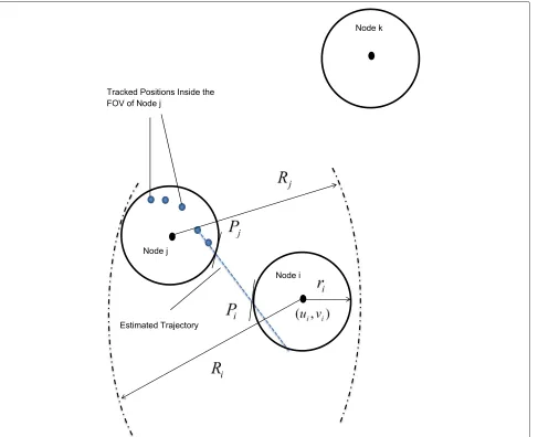
In the proposed approach, a WSN is composed of N nodes represented by the setNˆ = {n1,. . .,nN}. Each node has a known position(ui,vi) and a given sensing cover-age range which is simply modeled by circle with radiusri. All nodes within the communication rangeRican directly communicate withniand are referred to as neighbors. The number of neighbors ofniis given as ngh(ni). The avail-able resources of nodeniare modeled by a scalarEi. The battery power of sensor nodes is considered as resource. A set of tasks is considered to perform over time steps. Each task consumes some battery power from the energy budget of the sensor nodes. A set of static values for the energy consumption of tasks is considered. These values are assigned based on the energy demands of the task. A higher value is set for the tasks which need higher energy consumption.

The WSN application is composed of A tasks (or actions) represented by the set Aˆ = {a1,. . .,aA}. Once a task is started at a specific node, it executes for a spe-cific (short) period of time and terminates afterwards. Each task execution on a specific nodeni requires some resources E˜j and contributes to the overall application performance P. Thus, the execution of task aj on node ni is only feasible if Ei ≥ ˜Ej. The overall performance P is represented by an application-specific metric. On each node, an online task scheduling takes place which selects the next task to execute among theA-independent tasks. The task execution time is abstracted as a fixed period. Thus, scheduling is required at the end of each period which is represented as time instant ti. Non-preemptive scheduling is considered based on our pro-posed model. Figure 1 shows our considered WSN model components.

Table 1 shows the notations and meanings used to rep-resent the network model. The task scheduling approach is demonstrated using a target tracking application. A sen-sor network may consist of a variable number of nodes. The sensing region of each node is called the field of view (FOV). Every node aims to detect and track all targets in the FOV. If the sensor nodes would perform tracking all the time, then this would result in the best tracking performance. But executing target tracking all the time is energy demanding. Thus, a task should only be executed when necessary and sufficient for tracking performance. Sensor nodes can cooperate with each other by informing neighboring nodes about “approaching” targets. Neigh-boring nodes can therefore become aware of approaching targets.

(5)

Fig. 1WSN model components. There are four nodesni,nj. . .nk, andnl.Riis the communication range,riis the sensing range, and(ui,vi)is the position of the nodeni. Number of neighbors of the nodeni,ngh(ni)=2

is minimized. Naturally, these are conflicting optimization criteria, so there is no single best solution. The set of non-dominating solutions for such a multi-criteria problem can be typically represented by a Pareto front.

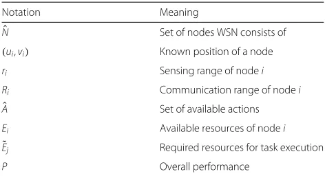
Table 1Notations used to represent the network model

Notation Meaning

ˆ

N Set of nodes WSN consists of

(ui,vi) Known position of a node

ri Sensing range of nodei

Ri Communication range of nodei

ˆ

A Set of available actions

Ei Available resources of nodei

˜

Ej Required resources for task execution

P Overall performance

4 System model

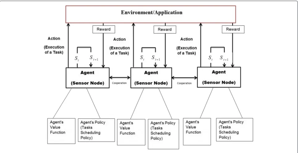
The task scheduler operates in a highly dynamic environ-ment, and the effect of the task ordering on the overall application performance is difficult to model. We con-sider the set of tasks, set of states, and the reward function as considered in [23]. Figure 2 depicts the scheduling framework where its key components can be described as follows:

• Agent: Each sensor node embeds an agent which is responsible for executing the online learning algorithm.

• Environment: The WSN application represents the environment in our approach. Interaction between the agent and the environment is achieved by executing actions and receiving a reward function. • Action: An agent’s action is the currently executed

(6)

Fig. 2General framework for task scheduling using online learning

each time periodti, each node triggers the scheduler to determine the next action to execute.

• State: A state describes an internal abstraction of the application which is typically specified by some system parameters. In our target tracking application, the states are represented by the number of currently detected targets in the node’s FOV and expected arrival times of targets detected by neighboring nodes. The state transitions depend on the current state and action.

• Policy: An agent’s policy determines what action will be selected in a particular state. In our case, this policy determines which task to execute at the perceived state. The policy can focus more on exploration or exploitation depending on the selected setting of the learning algorithm.

• Value function: This function defines what is good for an agent over the long run. It is built upon the reward function values over time, and hence, its quality totally depends on the reward function [7]. • Reward function: This function provides a mapping

of the agent’s state and the corresponding action to a reward value that contributes to the performance. We apply a weighted reward function which is capable of expressing the trade-off between energy consumption and tracking performance.

• Cooperation: Information exchange is considered among neighboring nodes as cooperation. The received information may influence the application’s state of sensor nodes.

5 Existing methods for task scheduling

Existing methods DIRL, RL, and CRL are described below. Each method is described briefly with the learning mech-anism and considered set of states and tasks.

5.1 DIRL

Shah and Kumar [7] use distributed independentQ learn-ing (DIRL) as reinforcement learnlearn-ing. The advantage of using independent learning is that no communication is required for coordination between sensor nodes and each node selfishly tries to maximize its own rewards. In Q learning, every agent needs to maintain aQmatrix for the value functions. Initially, all entries of theQmatrix are 0 and the agent of the nodes may be in any state. Based on the application-defined variables, the system goes to a par-ticular state. Then it performs an action which depends on the status of the nodes.

It calculates theQvalue for this (state, action) pair as

Qt+1(st,at)=(1−α)Qt(st,at)+α(rt+1(st+1)+γVt(st+1)), (1)

Vt+1(st)=max

a∈AQt+1(st,a) (2)

(7)

max

a∈AQt+1(st,a) means the maximumQ value after per-forming an action from the action setAfor the agenti.γ is the discount factor which can be set to a value in [0, 1]. For higherγ values, the agent relies more on the future than the immediate reward.αis the learning rate param-eter which can be set to a value in [0, 1]. It controls the rate at which an agent tries to learn by giving more or less weight to the previously learned utility value. Whenα is close to 1, the agent gives more priority to the previously learned utility value.

Algorithm 1 depicts the RL algorithm.

Algorithm 1Qlearning for task scheduling.

1: InitializeQ(s,a)= 0. Wheresis the set of states and ais the set of actions

2: whileResidual energy is larger than zerodo

3: Determine current statesby application variables 4: Select an actionawhich has the highestQvalue 5: Execute the selected action

6: CalculateQvalue for the executed action (Eq. 1) 7: Calculate the value function for the executed

action (Eq. 2)

8: Shift to next state based on the executed action 9: end while

5.2 RL

Khan and Rinner [8] propose cooperativeQlearning (RL) where every agent needs to maintain aQmatrix for the value functions like independentQlearning. Initially, all entries of theQmatrix are 0 and the nodes or agents may be in any state. Based on the application-defined variable or system variables, the system goes to a particular state. Then it performs an action which depends on the status of the nodes (example: For transmit action, a node must have residual energy which is greater than transmission cost). It calculates theQvalue for this (state, task) pair with the immediate reward. the immediate reward after executing the actionaat time t.Vtis the value function at timet.Vt+1is the value func-tion at timet+1. max

a∈AQt+1(st,a)means the maximumQ value after performing an action from the action setA.γ is the discount factor which can be set to a value in [ 0, 1]. The higher the value, the greater the agent relies on future reward than the immediate reward.αis the learning rate

parameter which can be set to a value in [0, 1]. It controls the rate at which an agent tries to learn by giving more or less weight to the previously learned utility value. When α is set close to 1, the agent gives more priority to the previously learned utility value.

f is the weight factor [24] for the neighbors of agenti and can be defined as follows:

f = 1 ngh(ni)

if ngh(ni)=0 (5)

f =1 otherwise. (6)

The algorithm can be stated as follows:

Algorithm 2Qlearning for task scheduling.

1: InitializeQ(s,a)= 0. Wheresis the set of states and ais the set of actions

2: whileResidual energy is not equal to zerodo

3: Determine current statesby application variables 4: Select an actionawhich has the highestQvalue 5: Execute the selected action

6: CalculateQvalue for the executed action (Eq. 3) 7: Calculate the value function for the executed

action (Eq. 4)

8: Send the value function to the neighbors 9: Shift to next state based on the executed action 10: end while

5.3 CRL

Khan and Rinner [9] applySARSA(λ)(CRL), also referred to as State-Action-Reward-State-Action, which is an iter-ative algorithm that approximates the optimal solution. SARSA(λ)[22] is an iterative algorithm that approximates the optimal solution without knowledge of the transition probabilities which is very important for a dynamic system like WSN. At each statest+1of iterationt+1, it updates Qt+1(s,a), which is an estimate of theQfunction by com-puting the estimation errorδtafter receiving the reward in the previous iteration. TheSARSA(λ)algorithm has the following updating rule for theQvalues:

Qt+1(st,at)←Qt(s,a)+αδtet(st,at) (7)

for alls,a.

In Eq. 7,α ∈[0, 1] is the learning rate which decreases with time. δt is the temporal difference error which is calculated by following rule

(8)

factor [24] for the neighbors of agentiand can be defined

An important aspect of an RL framework is the trade-off between exploration and exploitation [25]. Exploration deals with randomly selecting actions which may not have higher utility in search of better rewarding actions, while exploitation aims at the learned utility to maximize the agent’s reward.

A simple heuristic is used where exploration probability at any point of time is given by

=min(max,min+k∗(Smax−S)/Smax) (11)

wheremaxandmindenote upper and lower boundaries for the exploration factor, respectively. Smax represents maximum number of states which is three in our work, andSrepresents current number of states already known. At each time step, the system calculates and generates a random number in the interval of [0, 1]. If the selected random number is less than or equal to , the system chooses a uniformly random task (exploration); otherwise, it chooses the best task usingQvalues (exploitation).

SARSA(λ)improves learning through eligibility traces. et(s,a)is the eligibility traces in Eq. 7. Here,λis another learning parameter similar to α for guaranteed conver-gence.γ2is the discount factor. In general, eligibility traces give a higher update factor for recently revisited states. This means that the eligibility trace for a state-action pair (s,a)will be reinforced ifst ∈ sandat ∈a. Otherwise, if the previous actionatis not greedy, the eligibility trace is cleared.

Algorithm 3 SARSA(λ) learning algorithm for target tracking application.

1: InitializeQ(s,a)=0 ande(s,a)=0

3: Determine current statesby application variables 4: Select an action a, using policy

5: Execute the selected action

6: Calculate reward for the executed action (Eq. 38) 7: Update the learning rate (Eq. 14)

8: Calculate the temporal difference error (Eq. 8) 9: Update the eligibility traces (Eq. 13)

10: Update the Q-value (Eq. 7)

The eligibility trace is updated by the following rule:

et(st,at)=γ2λet−1(st,at)+1 ifst∈sandat∈a(12) et(st,at)=γ2λet−1(st,at) otherwise. (13)

The learning rateα is decreased slowly in such a way that it reflects the degree to which a state-action pair has been chosen in the recent past. It is calculated as

α= ζ

visited(s,a) (14)

whereζ is a positive constant and visited(s,a)represents the visited state-action pairs so far [26].

6 Proposed method for task scheduling

Following set of actions, set of states and reward function are considered for the proposed RATS.

6.1 Set of actions

The following actions are considered in our target track-ing application:

1. Detect_Targets: This function scans the field of view (FOV) and returns the number of detected targets in the FOV.

2. Track_Targets: This function keeps track of the targets inside the FOV and returns the current 2D positions of all targets. Every target within the FOV is assigned with a unique ID number.

3. Send_Message: This function sends information about the target’s trajectory to neighboring nodes. The trajectory information includes (i) the current position and time of the target and (ii) the estimated speed and direction. This function is executed when the target is about to leave the FOV.

4. Predict_Trajectory: This function predicts the velocity of the trajectory. A simple approach is to use the two most recent target positions, i.e.,(xt,yt)at timettand(xt−1,yt−1)attt−1. Then the constant target’s speed can be estimated as

v=

(xt−xt−1)2+(yt−yt−1)2/(tt−tt−1) (15) 5. Intersect_Trajectory: This function checks whether

the trajectory intersects with the FOV and predicts the expected time of the intersection. This function is executed by all nodes which receive the “target trajectory” information from a neighboring node. Trajectory intersection with the FOV of a sensor node is computed by basic algebra. The expected time to intersect the node is estimated by

˜

ti=DPiPj/v (16)

(9)

trajectory’s intersection points with the FOV of node i (cp. Fig. 3). v is the estimated velocity as calculated by Eq. 15.

6. Goto_Sleep: This function shuts down the sensor node for a single time period. It consumes the least amount of energy of all available actions.

The advanced trajectory prediction and intersection are considered for these methods. Inputs for this pre-diction task are the last few tracked positions of the target. Here, the last six tracked positions of the target are considered based on simulation stud-ies. The trajectory is linearized given by the last six tracked positions of the target considering the con-stant speed and direction. The speed is calculated by Eq. 15.

Suppose(x1,y1),(x2,y2). . .(xn,yn)are tracked positions of the moving object inside the FOV of the sensor node at time stepst1,t2. . .tn.

The trajectory can be predicted by the regression line [27] in Eq. 17:

y=bx+a+ (17)

wherebis the slope,ais the intercept, andis the residual or error for the calculation.

So residual,, can be calculated by following

i=yi−bxi−a (18)

wherei=1, 2, 3,. . .,n.

If the squares of the residuals of all the points from the line are summed up, what we get is a measure of the fitness of the line. The aim is to minimize this value.

(10)

So, the square of the residual is as follows: 2

i =(yi−bxi−a)2 (19)

To calculate the sum of square residuals, all the indi-vidual square residuals are added together as follows:

J= n

i=1

(yi−bxi−a)2 (20)

whereJis the sum of square residuals andnis the number of considered points.

Jin Eq. 20 needs to be minimized. The minimum value forJhas to occur when the first derivative is 0. The partial derivatives forJare with respect to the two parameters of the regression linebanda. To get the minimum, it needs to assign 0 [28].

Equations 21 and 22 can be shuffled and divided as n

Some constants can be pulled out in front of the summa-tions. Then_i₌₁acan be written as na in Eq. 23. We take the values of unknown parametersaandbusing Eqs. 23 and 24. These give two equations as follows:

b

Now, from Eqs. 25 and 26, some simple substitutions between the two equations are obtained as follows:

a= These formulas in Eqs. 27 and 28 do not tell us how pre-cise the estimates are. That is, how much the estimatorsa andbcan deviate from the “true” values ofaandb. It can be solved by confidence intervals.

Using Student’s t-distribution with (n−2) degrees of freedom [29], a confidence interval can be constructed for aandbas follows: example, ifτ = 0.05, the confidence level becomes 95 %. saandsbare the standard deviations as follows:

sb=

wherex¯is the average of thexvalues.

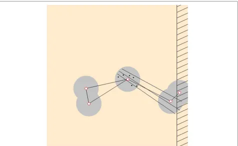
In Fig. 4, some tracked positions of the target are observed which is denoted by the “black” dots. At first, the regression line is predicted and the middle line is obtained. Then the confidence band is calculated which gives two other lines.

For the intersection with the circles, the line as follows is considered:

y=bx+a (33)

wherebis the slope andais the intercept.

The line given by Eq. 33 intersects a circle (sensing range is considered as a circle) given by Eq. 34:

(x−u1)2+(y−v1)2=r12 (34)

where(u1,v1)is the center andr1is the radius of the circle. Substituting the value of Eq. 33 in Eq. 34 gives the following:

(x−u1)2+((bx+a)−v1)2=r21 (35)

Simply expanding Eq. 35 by algebraic formula gives a quadratic equation of x and can be solved using the quadratic formula.

(11)

Fig. 4Trajectory prediction and intersection.Black dotsdenote the tracked positions of a target. Themiddle lineis drawn based on linear regression. Theother two linesare drawn by confidence interval

6.2 Set of states

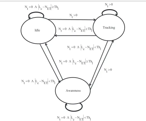
The application is abstracted by three states at every node.

• Idle: This state indicates that there is currently no target detected within the node’s FOV and the local clock is too far from the expected arrival time of any target already detected by some neighbor. If the time gap between the local clockLcand the expected arrival timeNETis greater than or equal to a threshold Th1(cp. Fig. 5), then the node remains in the idle state. The threshold Th1is set to 5 based on our simulation studies. In this state, the sensor node performsDetect_Targets less frequently to save energy.

• Awareness: There is currently also no detected target in the node’s FOV in this state. However, the node has received some relevant trajectory information, and the expected arrival time of at least one target is in less than Th1clock ticks. In this state, the sensor node performsDetect_Targets more frequently, since at least one target is expected to enter the FOV. • Tracking: This state indicates that there is currently

at least one detected target within the node’s FOV. Thus, the sensor node performs tracking frequently to achieve high tracking performance.

Obviously, the frequency of executing Detect_Targets andTrack_Targetsdepends on the overall objective, i.e., whether to focus more on tracking performance or energy consumption. The states can be identified by two appli-cation variables, i.e., the number of detected targets at the current timeNtand the list of arrival times of targets expected to intersect with node NET. Nt is determined by the task Detect_Targetswhich is executed at time t. If the sensor node executes the task Detect_Targets at timet, thenNtreturns the number of detected targets in the FOV. Each node maintains a list of appearing targets and the corresponding arrival time. Targets are inserted in this list if the sensor node receives a message and the estimated trajectory intersects with the FOV. Targets are removed if a target is detected by the node or the expected arrival time with an additional threshold Th1has expired.

(12)

Fig. 5State transition diagram. States change according to the value of two application variablesNtandNET.Lcrepresents the local clock value, and Th1is a time threshold

quality. But this situation could provide better energy effi-ciency, since theTrack_Targetstask consumes the highest amount of energy among all the tasks. So, selection of a particular task at each time step or scheduling of tasks provides an impact on overall tracking quality/energy consumption trade-off.

Figure 5 depicts the state transition diagram where Lc is the local clock value of the sensor node and Th1 represents the time threshold betweenLcandNET.

6.3 Reward function

The reward function is a key system component for expressing the effect of the task execution on the sys-tem performance and resource consumption. Thus, both aspects should be covered by the reward function. Among the various options, it is simplified by merging energy

consumption and system performance using a balancing parameter. In detail, the reward function in our algorithm is defined as

r=β(Ei/Emax)+(1−β)(Pt/P) (38)

(13)

6.4 Proposed method

The classical adversarial algorithm Exp3 (exponential-weight algorithm for exploration and exploitation) is used for task scheduling [6].

Algorithm 4Task Scheduling by Bandit Solver Exp3. 1: Parameters: Number of tasks A, Factorκ ≤1 2: Initialization: wi,0 = 1 and Pi,1 = 1/A for i =

1, 2,. . .,A

4: Determine current s based on application variables

5: Select an actiona∈ {1, 2,. . .,A}based on thePt 6: Execute the selected action

7: Calculate the reward (Eq. 41) 8: Update the weights (Eq. 40)

9: Calculate the updated probability distribution (Eq. 39)

Exp3 has a parameterκ which controls the probability with which arms are explored in each round. At each time stept, Exp3 draws an actionaaccording to the distribu-tionP1,t,P2,t,. . .,PA,t. The distribution can be calculated

where wa,t is the weight associated with the actionaat timet.

This distribution is a mixture of the uniform distribu-tion and a distribudistribu-tion which assigns to each acdistribu-tion a probability mass exponential in the estimated reward for that action. Intuitively, mixing in the uniform distribution is done to make sure that the algorithm tries out all actions Aand gets good estimates of the rewards for each action.

Weight for each action can be calculated by following equation

wa,t=wa,t−1eκrt+1 (40)

wherert+1is the reward after executing the actiona. Reward can be calculated by following equation

rt+1= rt Pa,t

(41)

wherePa,tis the calculated probability distribution for the actionaby Eq. 39.

Exp3 works by maintaining a list of weightswiby Eq. 40 for each of the actions, using these weights to decide which action to take next based on a probability distri-butionPt, and increasing the relevant weights when the

reward is positive. The egalitarianism factor κ ∈[0, 1] tunes the desire to pick an action uniformly at random. If κ = 1, the weights have no effect on the choices at any step.

7 Experimental results and evaluation

7.1 Simulation environment

The proposed method is implemented and evaluated with other task scheduling methods using a WSN multi-target tracking scenario implemented in a C# simulation envi-ronment.

The simulator consists of two stages: the deployment of the nodes and the execution of the tracking appli-cation. In the evaluation scenario, the sensor nodes are uniformly distributed in a 2D rectangular area. A given number of sensor nodes are placed randomly in this area which can result in partially overlapping FOVs of the nodes. However, placement of nodes on the same posi-tion is avoided. Before deploying the network, the network parameters should be configured using the configuration sliders.

The following network parameters can be configured by our simulator.

• Network size: Network size means the number of nodes in the network. In the current settings of the simulator, the number of sensor nodes can be varied between [3, 40].

• Sensor radius: Sensor radius is the sensing range of the sensors in the network. Sensor radius can be varied between [1, 50].

• Transmission radius: Transmission radius is the maximum distance within two sensor nodes communicating with each other. If it is set to a high value, nodes on the opposite side of the rectangular area may be able to reach each other. If it is set to a low value, nodes must be very close to communicate with each other. Transmission radius can be varied between [1, 50].

(14)

Targets move around in the area based on a Gauss-Markov mobility model [30]. The Gauss-Gauss-Markov mobility model was designed to adapt to different levels of random-ness via tuning parameters. Initially, each mobile target is assigned with a current speed and direction. At each time stept, the movement parameters of each target are updated based on the following rule:

St=ηSt−1+(1−η)S+

where St and Dt are the current speed and direction of the target at time t, respectively. S and D are con-stants representing the mean value of speed and direction, respectively.S_tG₋₁andDG_t₋₁ are random variables from a Gaussian distribution.ηis a parameter in the range [ 0, 1] and is used to vary the randomness of the motion. Ran-dom (Brownian) motion is obtained ifη = 0, and linear motion is obtained ifη = 1. At each timet, the target’s position is given by the following equations:

xt=xt−1+St−1cos(Dt−1) (44)

yt=yt−1+St−1sin(Dt−1) (45)

7.2 Settings of parameters

In the simulation, we limit the number of concurrently available targets to seven. The total energy budget for each sensor node is considered as 1000 units. Table 2 shows the energy consumption for the execution of each action. Sending messages over two hops consumes energy on both the sender and relay nodes. To simplify the energy consumption at the network level, only the energy con-sumption to ten units on the sending node only is aggre-gated. The egalitarianism factorκ = 0.5 is set for Exp3. The sensing radius is considered asri = 5, and the com-munication radius is set as Ri = 8. These fixed values are set for the parameters based on simulation studies. For each simulation run, the achieved tracking quality and energy consumption are aggregated and normalized to [0, 1].

Table 2Energy consumption of the individual actions

Action Energy consumption (unit)

For the evaluation, the following four experiments are performed with the following assumptions of parameters.

1. To find out the trade-off between tracking quality and energy consumption, the balancing factorβof the reward function is set between[0.1, 0.9]in 0.1 steps, keeping the randomness of moving target as η=0.5, setting the egalitarianism factor of Exp3 as κ =0.5, and fixing the topology to five nodes. 2. The network size is varied to check the trade-off

between tracking quality and energy consumption. Three different topologies consisting of 5, 10, and 20 sensor nodes are considered where the coverage ratio is 0.0029, 0.0057, and 0.0113, respectively. The coverage ratio is defined as the ratio of the aggregated FOV of all deployed sensor nodes over the area of the entire surveillance area. The balancing factor is set β =0.5and the randomness of the mobility model η=0.5which is a constant for this experiment. 3. Randomness of moving targetsηis set to one of the

following values

{0.1, 0.15, 0.2, 0.25, 0.3, 0.4, 0.5, 0.7, 0.9}and setting the balancing factorβ=0.5and fixing the topology to five nodes.

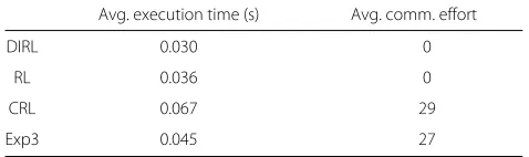
4. DIRL, RL, CRL, and Exp3 are evaluated in terms of average execution time and average communication effort. These values are measured from 20 iterations and represent the mean execution times and the mean ofSend_Message task executions.

7.4 Discussion

Figure 6 shows the results of our first experiment. Each data point in these figures represents the average of normalized tracking quality and energy consumption of ten complete simulation runs. The results show the track-ing quality/energy consumption trade-off for DIRL, RL, CRL, and Exp3 by varying the balancing factorβbetween [0.1, 0.9] in 0.1 steps. It is observed that CRL and Exp3 provide similar results, i.e., the corresponding data points are closely co-located. RL is energy-aware but is not able to achieve high tracking quality. DIRL achieves the most energy awareness but provides the least tracking quality.

(15)

Fig. 6Tracking quality/energy consumption trade-off for DIRL, RL, CRL, and Exp3 by varying the balancing factor of the reward function_β

Figures 8, 9 and 10 show the results of our third exper-iment. In this experiment, each data point represents the average of normalized tracking quality and the energy consumption of ten complete simulation runs by vary-ing the randomness of movvary-ing objectsηto one of these values{0.10, 0.15, 0.20, 0.25, 0.30, 0.40, 0.50, 0.70, 0.90}for each method. From these figures, it can be seen that CRL and Exp3 outperform RL and DIRL in terms of achieved tracking performance. It can be seen that for lower randomness, η = 0.5, 0.7, and 0.9, RL and Exp3 show very close results for tracking performance. But for higher randomness, η = 0.1, 0.15, and 0.2, DIRL gives poor performance with regard to tracking performance.

Table 3 shows the comparison of DIRL, RL, CRL, and Exp3 in terms of average execution time and average communication effort. These values are derived from 20 iterations and represent the mean execution times and

the mean ofSend_messagetask executions. It can be seen that DIRL and RL are resource-aware in terms of execu-tion time and communicaexecu-tion effort. Exp3 requires 25 % more and CRL requires 86 % more execution time. The communication overhead is similar for both Exp3 and CRL.

8 Conclusions

In this paper, an adversarial bandit solver is applied based on online learning algorithm for resource-aware task scheduling in WSN. The performance of our pro-posed online task scheduling method is evaluated with other existing task scheduling methods based on the three learning algorithms: DIRL, RL, and CRL. Evaluation results show that our proposed RATS method provides better performance in terms of tracking quality. DIRL shows the best energy efficiency but provides poor results in terms of tracking quality. The proposed RATS and CRL

(16)

Fig. 8Tracking quality/energy consumption trade-off for DIRL, RL, CRL, and Exp3 with different randomness of target movements,η=0.10, 0.15, and 0.20

Fig. 9Tracking quality/energy consumption trade-off for DIRL, RL, CRL, and Exp3 with different randomness of target movements,η=0.25, 0.30, and 0.40

(17)

Table 3Comparison of average execution time and average number of transferred messages (based on 20 iterations)

Avg. execution time (s) Avg. comm. effort

DIRL 0.030 0

RL 0.036 0

CRL 0.067 29

Exp3 0.045 27

show almost similar results in terms of tracking quality-energy consumption trade-off. Evaluation results show that these methods provide different properties concern-ing achieved performance and resource awareness. The selection of a particular algorithm depends on the appli-cation requirements and the available resources of sensor nodes.

Future work includes the application of our resource-aware scheduling approach to different WSN applications, the implementation on our visual sensor network plat-forms [31], and the comparison of our approach with other variants of reinforcement learning methods.

Competing interests

The author declares that he has no competing interests.

Received: 8 October 2015 Accepted: 28 December 2015

References

1. L Xiang, J Luo, A Vasilakos, “Compressed data aggregation for energy efficient wireless sensor networks,” in Sensor, Mesh and Ad Hoc Communications and Networks (SECON), 2011 8th Annual IEEE Communications Society Conference on, june 2011, 46–54 (2011) 2. Y Song, L Liu, H Ma, AV Vasilakos, A biology-based algorithm to minimal

exposure problem of wireless sensor networks. IEEE Trans. Netw. Serv. Manag.11(3), 417–430 (2014)

3. AV Vasilakos, GI Papadimitriou, A new approach to the design of reinforcement schemes for learning automata: stochastic estimator learning algorithm. Neurocomputing.7(3), 275–297 (1995) 4. L Liu, Y Song, H Zhang, H Ma, AV Vasilakos, Physarum optimization: a

biology-inspired algorithm for the Steiner tree problem in networks. IEEE Trans. Comput.64(3), 819–832 (2015)

5. H Saad, A Mohamed, T ElBatt, Cooperative Q-learning techniques for distributed online power allocation in femtocell networks. Wirel. Commun. Mob. Comput (2014). doi:10.1002/wcm.2470

6. P Auer, NC Bianchi, Y Freund, RE Schapire, The nonstochastic multiarmed bandit problem. SIAM J. Comput.32, 48–77 (2003).

doi:10.1137/S0097539701398375

7. K Shah, M Kumar, inProceedings of IEEE Mobile Adhoc and Sensor Systems. Distributed Independent Reinforcement Learning (DIRL) Approach to Resource Management in Wireless Sensor Networks (IEEE, Pisa, Italy, 2007), pp. 1–9

8. MI Khan, B Rinner, inProceedings of the IEEE International Conference on Pervasive Computing and Communications Workshops. Resource Coordination in Wireless Sensor Networks by Cooperative Reinforcement Learning (IEEE, Lugano, Switzerland, 2012), pp. 895–900

9. M Khan, B Rinner, inProceedings of the IEEE International Conference on Communications Workshops. Energy-Aware Task Scheduling in Wireless Sensor Networks Based on Cooperative Reinforcement Learning (IEEE, Sydney, Australia, 2014), pp. 871–877

10. C Frank, K Römer, inProceedings of the ACM Conference on Embedded Networked Sensor Systems. Algorithms for Generic Role Assignments in Wireless Sensor Networks (IEEE, San Diego, California, 2005), pp. 230–242

11. JHW Ye, D Estrin, inProceedings of the INFOCOM’02. An Energy-Efficient MAC Protocol for Wireless Sensor Networks (IEEE, New York, USA, 2002), pp. 1567–1576

12. Y Tian, E Ekici, F Ozguner, inProceedings of the IEEE International Conference on Mobile Adhoc and Sensor Systems Conference. Energy-constrained Task Mapping and Scheduling in Wireless Sensor Networks (IEEE, Washington, DC, 2005), pp. 210–218

13. T He, S Krishnamurthy, JA Stankovic, T Abdelzaher, L Luo, R Stoleru, T Yan, L Gu, inIn Mobisys. Energy-Efficient Surveillance System Using Wireless Sensor Networks (ACM Press, 2004), pp. 270–283

14. W Guo, N Xiong, H-C Chao, S Hussain, G Chen, Design and analysis of self adapted task scheduling strategies in WSN. Sensors J.11, 6533–6554 (2011). doi:10.3390/s110706533

15. X Xu, R Ansari, A Khokhar, AV Vasilakos, Hierarchical data aggregation using compressive sensing (HDACS) in WSNs. ACM Trans. Sens. Netw.

11(3), 1–25 (2015)

16. S Giannecchini, M Caccamo, CS Shih, inProceedings of the Euromicro Conference on Real-Time Systems. Collaborative Resource Allocation in Wireless Sensor Networks (IEEE, Rennes, France, 2004), pp. 35–44 17. T Meng, F Wu, Z Yang, G Chen, AV Vasilakos, Spatial reusability-aware

routing in multi-hop wireless networks. IEEE Trans. Comput., 1–13 (2015). doi:10.1109/TC.2015.2417543

18. B Krishnamachari, S Wicker, R Bejar, C Fernandez, “On the complexity of distributed self-configuration in wireless networks”. J. Telecommun. Syst.

22(1–4), 33–59 (2003)

19. C Busch, R Kannan, AV Vasilakos, Approximating congestion + dilation in networks via “Quality of Routing” games. Int. J. Distrib. Wirel. Sens. Netw.

61(9), 22 (2014)

20. S Dhanani, J Arseneau, A Weatherton, B Caswell, N Singh, S Patek, in Proceedings of the IEEE Systems and Information Engineering Design Symposium. A Comparison of Utility Based Information Management Policies in Sensor Networks (IEEE, Charlottesville, Virginia USA, 2006), pp. 84–89

21. P Li, S Guo, S Yu, AV Vasilakos, inProceedings of the IEEE INFOCOM. CodePipe: An opportunistic feeding and routing protocol for reliable multicast with pipelined network coding, (Orlando, FL, 2012), pp. 100–108 22. RS Sutton, AG Barto,Reinforcement Learning: An Introduction. (MIT Press,

Cambridge, Massachusetts, United States, 1998)

23. MI Khan, B Rinner, Performance analysis of resource aware task scheduling methodologies in wireless sensor networks. International Journal of Distributed Sensor Networks, Hindawi, Volume 2014, 11 (2014) 24. KLA Yau, P Komisarczuk, PD Teal, Reinforcement learning for context

awareness and intelligence in wireless networks: review, new features and open issues. J. Netw. Comput. Appl.35, 253–267 (2012) 25. J Byers, G Nasser, inProceedings of the Workshop on Mobile and Ad Hoc

Networking and Computing. Utility Based Decision making in Wireless Sensor Networks (IEEE, Boston, MA, 2000), pp. 143–144

26. RAC Bianchi, CHC Ribeiro, AHR Costa,Advances in Artificial Intelligence. (Springer, Berlin, Germany, 2004)

27. DC Montgomery, EA Peck, GG Vining,Introduction to Linear Regression Analysis. (Wiley, Hoboken, New Jersey, United States, 2007), p. 152 28. N Bery, Linear regression. Technical report. DataGenetics (2009) 29. MR Spiegel,Theory and Problems of Probability and Statistics. (McGraw-Hill,

New York City, New York, United States, 1992), pp. 116–117

30. T Abbes, S Mohamed, K Bouabdellah, Impact of model mobility in ad hoc routing protocols. Comput. Netw. Inf. Secur.10, 47–54 (2012)