Volume 2009, Article ID 656832,12pages doi:10.1155/2009/656832
Research Article
An Active Constraint Method for Distributed Routing, and
Power Control in Wireless Networks
Alban Ferizi,
1Armin Dekorsy,
2Joerg Fliege,
3Larissa Popova,
4Wolfgang Koch,
4and Michael S¨ollner
51Institute for Electronics Engineering, University Erlangen-Nuremberg, Cauerstraße 9, 91058 Erlangen, Germany 2Qualcomm CDMA Technologies GmbH, Nordostpark 89, 90411 Nuremberg, Germany
3CORMSIS, School of Mathematics, University of Southampton, University Road, Southampton, SO17 1BJ, UK 4Chair of Mobile Communications, University Erlangen-Nuremberg, Cauerstraße 7, 91058 Erlangen, Germany 5Alcatel-Lucent, Thurn-und-Taxis-Straße 10, 90411 Nuremberg, Germany
Correspondence should be addressed to Alban Ferizi,[email protected]
Received 17 April 2009; Revised 21 September 2009; Accepted 15 December 2009
Recommended by Alex B. Gershman
Efficiently transmitting data in wireless networks requires joint optimization of routing, scheduling, and power control. As opposed to the universal dual decomposition we present a method that solves this optimization problem by fully exploiting our knowledge of active constraints. The method still maintains main requirements such as optimality, distributed implementation, multiple path routing and per-hop error performance. To reduce the complexity of the whole problem, we separate scheduling from routing and power control, including it instead in the constraint set of the joint optimization problem. Apart from the mathematical framework we introduce a routing and power control decomposition algorithm that uses the active constraint method, and we give further details on its distributed application. For verification, we apply the distributed RPCD algorithm to examples of wireless mesh backhaul networks with fixed nodes. Impressive convergence results indicate that the distributed RPCD algorithm calculates the optimum solution in one decomposition step only.
Copyright © 2009 Alban Ferizi et al. This is an open access article distributed under the Creative Commons Attribution License, which permits unrestricted use, distribution, and reproduction in any medium, provided the original work is properly cited.
1. Introduction
Nowadays, there is an increased interest in communication via wireless mesh networks such as ad-hoc, sensor, or wireless mesh backhauling networks [1,2]. In wireless networks the link capacities are variable quantities and can be adjusted by the resource allocation such as scheduling, and power allo-cation to fully exploit network performance. Hence, for effi -cient data transmission an integrated routing, time schedul-ing and power control optimization strategy are required. This strategy has to take different transmission constraints into account, for example, maximum available power level or limited buffer size at nodes. The inherent decentralized nature of wireless mesh networks mandates that distributed algorithms should be developed to implement the joint routing, scheduling, and power control optimization. The first step towards a distributed implementation is to break up this problem into manageable subproblems and solve these
dual problem coordinates them. In this paper we con-sider joint routing, time-scheduling, and power control for single frequency wireless mesh networks. The wireless transmissions are arranged in time-slots. However, we take into account that simultaneously active transmissions suffer from multiple access interference. Dual decomposition is a universal approach to solve such optimization problems [5,6], but it does not consider the specific combinational structures of optimization problems. By contrast, we propose a novel method that explicitly exploits the combinational structure of a joint routing, time-scheduling, and power control problem by means of an active constraint method. The formulation of the optimization problem is yet generally valid, so that the method proposed here is applicable to a plurality of wireless networks. The proposed approach meets the following requirements: (1) less iterations to an optimum solution, (2) distributed implementation, (3) multiple path routing, and (4) per hop error performance. In particular, the approach is as follows. We separate scheduling from routing and power allocation by including it in the constraint set of a Simultaneous Routing and Power Control (SRPC) problem. For scheduling, several well known approximations such as Greedy-based approaches exist [7, Section 3.7], that we can leverage on. The constraints we use in the SRPC problem are induced by a precalculated colored graph of the network that, in turn, reflects the scheduling decisions of any arbitrary scheduler. Consequently, the main contribution is to introduce a Routing and Power Control Decomposition (RPCD) method to solve the simultaneous routing and power control problem while meeting the above-mentioned requirements. The clever bits of the RPCD are manifold. (1) We rewrite the SRPC problem to an equivalent problem by applying the active constraint method. (2) We decouple the equivalent problem by solving a (convex) network and a (convex) power assignment problem separately. (3) Iterations are performed by switching between the two subproblems for which network and power variables act as interchanging variables. Apart from the mathematical framework we introduce the RPCD algorithm and prove its convergence to a KKT-point of the joint routing and power control problem. We compare the RPCD algorithm with dual decomposition as state-of-art approach with respect to the number of iterations needed to calculate the KKT-point. This verification is performed by applying both algorithms to a wireless cellular mesh backhauling network [1,2]. The backhauling network describes a “regular” cellular network. This models the situation where, in order to save infrastructure expenses of laying cable or fiber to each node (base station), we try to extend the range of a given source node with wired backhaul connection by using several other nodes. These intermediate nodes have no wired connection and can only communicate with the backhaul via the source node by wireless mesh communications. The simulation set-up correctly models mobile radio channel characteristics such as path-loss and slow fading. The comparison indicates that the RPCD approach requires only one decomposition step to calculate the optimum solution as opposed to dual decomposition. This paper is organized as follows. In Section 2 we describe the network model used for
the wireless data network. In Section 3 we formulate the optimization problem and define the standard interference function. The RPCD algorithm for solving the joint routing and power control problem is presented in Section 4. We extend the RPCD algorithm in Section 5 by introducing distributed algorithms for solving the routing and power assignment problem. Finally, in Section 6 we apply the algorithm to a wireless backhaul network and present the simulation results. We conclude the paper inSection 7.
2. Network Model
The transmission problem we are facing is to transmit messages indexed bymeach of sizeSmin bits via a multiple
hop wireless network. Each message has its source nodesm
and its destination nodedm=/sm. LetMbe an index set for
the set of messages withm∈M. Withmultiple path routing
each message is transmitted via several paths from its source node to its destination node. Thus, nodes can send parts of messages to many receivers and receive parts of messages from many transmitters. We denote the nodes byv∈Vwith
V be a finite set of nodes. At any time, each of these nodes
v∈Vcan map any parts of messagesm∈Monto a single linkefor transmission. The set of all links is denoted byE. A wireless communication link corresponds to an edgee =
(u,v) between two nodesu,vand is described by the ordered pair (u,v)∈V×Vsuch thatutransmits information directly tov. Moreover, we assume that (v,v)∈/Efor allv ∈V. We have thatG := (V,E) is a directed graph with node set V
and edge set E. For an arbitrary node v ∈ V, denote by
E+(v) := {e ∈ E | e = (v,w) ∈ E}andE−(v) := {e ∈ E | e = (w,v) ∈ E} the set of outgoing and incoming edges withinEat the nodev, respectively. A link represents a wireless resource characterized by a given bandwidth, time duration, space fraction, or by a given code assignment. We assume a time-slotted single frequency network for which the time is divided into equal slots of length τ while all nodes occupy the same frequency band of bandwidth B. Time slots are indexed byt ∈ T, withT as an index set. We take time scheduling into account by assuming that there is a given coloring of the nodes such that adjacent nodes do not have the same color (half-duplex constraint) [4]. That is, we are given a number C and a function coV : V → {1,. . .,C} such that coV(v)=/coV(w) for all nodes v,w ∈ V with (v,w) ∈ E. Here, C is at least as large as the chromatic number ofG. Computing such a coloring can be done by a Greedy approach [7]. To take delay constraints into account we introduce tmax as the maximum number
of time slots, a message is allowed to use for transmission from its source to its destination, that is,T := {1,. . .,tmax}. The interference model we consider includes multiple access interference caused by simultaneously active transmissions that can not be perfectly separated by, for example, code- or space division multiple access (CDMA/SDMA) techniques. Thus, letEe,t be the set of edges interfering edgee at time t. The signal attenuation from nodeuto nodevisGt(u,v)
the corresponding senders. Let T(e) be the transmitting node and let R(e) be the receiving node of edge e. Hence,
Gt(T(l),R(e)) denotes the attenuation a signal suffers that is
transmitted fromT(l) but received by node R(e). For link
e such a signal represents multiple-access interference that is caused by linkl. Furthermore, with pe,tas the (transmit)
power to be allocated to linke at time slott, the received signal power at nodeR(e) from the transmitterT(e) is given by Gt(T(e),R(e))pe,t. We define the
signal-to-interference-plus-noise ratio (SINR) of edge e ∈ E at time slott ∈ T
as
SINRe,t= Gt
(T(e),R(e))pe,t
l∈Ee,t,l /=eGt(T(l),R(e))pl,t+σe2
(1)
with σ2
e as an additive noise power of edge e. If we only
assume thermal noise to be the same for all edges, we have σ2
e = BN0 with noise spectral density N0. For the
optimization problems to be introduced later we have the following design variables. As network flow variables we have
ce,m,t ∈Ras the part of the messagemsent along edgeein
time slott(in bits), andbv,m,t∈Ras the part of the message m stored in a buffer at node vdirectly before the start of time slott(in bits). Communication variablepe,t ∈Ris the
transmit power allocated to edgeeat time slottto transmit the total traffic on edgee(in Watt). If we stack the different variables to vectors we obtainc =(ce,m,t),b =(bv,m,t), and
p = (pe,t). We further use the following parameters. Let Sm ∈ R+ be the size of messagem(in bits) and Bv ∈ R+
be the maximum total buffer size at nodev(in bits). Power constraints are Pmax
v ∈ R+ as the maximum transmission
power of a node (in Watt) assumed to be the same for all nodes andPmax
e ∈R+as the maximum transmission power
per edge (in Watt).
3. Optimization Problem
3.1. Problem Description. Let us consider an operation of
a wireless data network with the objective to minimize a convex cost function f(p,c,b) (or to maximize a concave utility function). The design variablesb,c,andpare subject to some constraints. For instance, with (e∈E,m∈M,v∈
V,t∈T) we require the power constraints
pe,t≥0, (2)
pe,t≤Pmaxe , (3)
e∈E+(v)
pe,t≤Pmaxv (4)
forming the polyhedral set
Cp:=
p|pfulfills (2), (3), and (4). (5) Since we isolated coloring from the joint routing and power control, we have to take the precalculated colored network graph in the flow constraints into account. Similar to power constraints, we require that flow constraints form a polyhedral set Cc. For example, if we assume that given
source nodes sm have to transmit messages of sizes Sm to
destinations dm in a given timetmax, the polyhedral setCc
is defined by the equalities and inequalities
ce,m,t≥0 (e∈E,m∈M,t∈T), (6)
bv,m,t≥0 (v∈V,m∈M,t∈T), (7)
bv,m,t≤Bv,m (v∈V,m∈M,t∈T), (8)
bsm,m,1=Sm (m∈M), (9)
bv,m,1=0 (v∈V\ {sm},m∈M), (10)
bdm,m,tmax =Sm (m∈M), (11)
bv,m,tmax =0 (v∈V\ {dm},m∈M), (12)
ce,m,t=0 (m∈M, coE(e)=/coT(t)), (13) bv,m,t+1−bv,m,t=
e∈E−(v)
ce,m,t−
e∈E+(v)
ce,m,t,
(m∈M,v∈V,t∈T\ {tmax}).
(14)
Equations (7) and (8) avoid buffer overload while (9) and (10) initialize buffer values. To account for delay constraints (11) and (12) ensure that messages reach their destinations completely attmaxat last . Coloring is ensured by (13) and
(14) is a modified Kirchhoff’s Law [6]. The SRPC problem under consideration is now as follows
minimize fp,c,b
subject to (b,c)∈Cc
p∈Cp
m∈M
ce,m,t≤Re,t
p e∈E+(v), t∈T.
(15)
By the last constraints, we assume that at any timet∈T
each node v ∈ V can map all part of messages m ∈ M
onto a single linke∈Efor transmission [5]. Furthermore, we assume that the amount of information (in bits) we can transmit on a single wireless linkeat time slottis bounded from above by a maximum mutual information bound
Re,t(p) that itself depends on the power setting. The last
constraints of (15) are the only constraints coupling network flow variables (b,c) with communication variablesp. Thus, we call them coupling constraints [5], and they represent the most challenging constraints of the SRPC problem. All the other constraints are either constraints for the network flow variables or for the communication variables only. Assuming time-invariant channel conditions within the duration of a single time slott, functionRe,t(p) describes the amount of
information of edgeeand can be expressed with (1) by the well-known Shannon formula
Re,t
p=B·τ·log2
1 + 1
ΩeSINRe,t (e∈E,t∈T).
(16) For each edge e, the factor Ωe ∈ R+0 represents any
information given by the Shannon formula [8]. In practice, achieving this mutual information requires adaptive mod-ulation and coding. To accomplish the description of the optimization problem under consideration, we like to list some commonly used examples of cost (utility) functions. Examples are
(1) minimization of total transmitted power
fp=
e∈E,t∈T
pe,t, (17)
(2) maximization of total network throughput
f(c)=
v∈V
gv(c) (18)
with gv(c) representing any linear combination of
flows that egress nodev,
(3) any linear combination of items (1) and (2).
A comprehensive overview on commonly used cost functions for wireless data networks is given in [5].
3.2. Standard Interference Function. In the following we give
an interpretation of the coupling constraints (m∈Mce,m,t ≤ Re,t(p)) of the SRPC problem (15). We define fore∈Eand
t∈T
Je,t
p,c:=Ωe
2((m∈Mce,m,t)/B·τ)−1
Gt(T(e),R(e))
× ⎛
⎝
l∈Ee,t,l /=e
Gt(T(l),R(e))pl,t+σe2
⎞ ⎠
(19)
to be astandard interference functioninp[9]. To clarify the meaning of a standard interference function, we restate the definition given in [9]. Here,andmean componentwise inequality.
If we insert (1) into (16) and solve the coupling constraints in (15) for power values, we obtain rewritten coupling constraints as
pJp,c. (20)
Definition 1. For given valuesc,J(p,c) is astandard
inter-ference functionif for allp ≥0 the following properties are
satisfied.
(i)Positivity:J(p,c)0.
(ii)Monotonicity: ifppthenJ(p,c)J(p,c). (iii)Scalability: For allα >1,αJ(p,c)J(αp,c)
The positivity property ensures positive power values of the joint routing and power control problem (15). If any transmit power level is decreased, the monotonicity guarantees the decrease of the interference on the other links in the network, ensuring the maintenance of the same or even the achievement of a lower interference level for all
links. The scalability property implies that ifpJ(p,c) then
αpαJ(p,c)J(αp,c) forα >1.
Interestingly, (20) represents a Quality-of-Service (QoS) constraint, that is, a lower bound on the (implicitly defined) SINR. By reusing the coupling constraints again (15) and solving (16) for SINR we require
SINRe,t≥Ωe
2((m∈Mce,m,t)/B·τ)−1 (e∈E,m∈M,t∈T). (21) SINR is the main indicator for the transmission quality. Hence, given a modulation and coding scheme a specific per-hop error performance implies a respectiveΩe. In turn, by
varyingΩewe vary the transmission quality.
Note that for given valuesce,m,t ≥0, we can use a fixed
point iteration algorithm to find a unique power vectorp∗∈ RE×Twith
p∗=Jp∗,c. (22) This power iteration represents a standard power control algorithm as introduced in [9]. The power iteration used herein to solve (15) will be described in detail inSection 5.1. With coupling constraints (20) of problem (15) we can make use of the properties of the standard interference function [9], arriving at the following theorem.
Theorem 1. Suppose thatσ2
e >0 (e ∈ E), that the objective
function f : (p,b,c) → f(p,b,c)is monotone inp, and that we want to solve the optimization problem
minimize fp,c,b
subject to (b,c)∈Cc
p∈Cp
pJp,c.
(23)
Suppose there exists a feasible point of this optimization problem, then there exists a feasible point with the same or
better objective function value for which all the constraints(20)
are active, that is, equality holds in all of them. Especially, for every optimum objective function value there exists an
optimum variable setting such that all constraints in(20)are
active. If f is strictly monotone inp, then all constraints(20)
are active at each optimal solution of this problem.
Proof. SeeAppendix A.
Theorem 1 is an extension of the results found in [9]. In contrast to [9] we do not assume that f is just a sum of powers, instead it can be an arbitrary function being monotone in power values. Moreover, the objective as well as the coupling constraints depend on the flow variablesc
and buffersb, a case not considered in [9].
4. RPCD-Algorithm
Power allocation algorithm (distributed) Check for
stop Optimum
achieved
p∗,c∗,b∗
Interim power valuesp
Interim network valuesc,b
Feasible power valuespstart
Routing alogrithm (distributed)
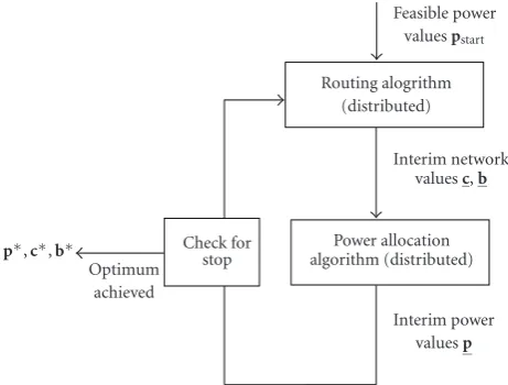
Figure1: RPCD Algorithm.
like the dual decomposition method, we fully exploit our knowledge of active constraints of the joint optimization problem.
Based on Theorem 1 we can formulate an equivalent optimization problem but we avoid the extension of the utility function as usually done by applying dual or penalty approaches. We further keep the constraints and we only have to exchange the common network and power variables. The main idea of the RPCD-Algorithm is to decouple the SRPC problem into two convex subproblems and to find the optimum solution of the SRPC problem by iteratively toggling between the two subproblems (Figure 1).
4.1. RPCD-Principle. Let us consider again problem (15).
Due to Theorem 1 we know that all coupling constraints (20) of the SRPC problem are active at least at one optimum solution. By means of this observation, we can rewrite the SRPC problem to an equivalent problem as follows. Activity (equality) means that
p=Jp,c. (24) We now substitute (24) into the objective of the SRPC problem (15) and obtain an equivalent problem with the rewritten cost function as
minimize fJp,c,c,b
subject to (b,c)∈Cc,
p∈Cp,
pJp,c.
(25)
In the following we use (25) and decompose the SRPC problem into two convex subproblems.
In particular, by assuming feasible power variables, a routing problem with fixed link capacities is formulated and the optimum flow variables for the routing problem are calculated. Equivalently, we can assume fixed routing variables and formulate a power control problem to calculate optimum power values [10].
The two subproblems are as follows.
4.1.1. Network Flow (Routing) Subproblem. We assume
feasi-ble power variafeasi-blesp ∈Cp. With (25) we need to solve the
optimization problem
minimize fJp,c,c,b
subject to (b,c)∈Cc,
m∈M
ce,m,t≤Re,t
p,
(26)
wherec,bare the optimization variables. We have the following lemma.
Lemma 1. (1) If f is a continuously differentiable and
monotone function in pand inc, then the objective of (26)
is a continuously differentiable and monotone function inc.
(2) Letσ2
e >0(e∈E). Suppose thatfis twice continuously
differentiable, thatf(·,b,c)is a convex and monotone function
inpfor all(b,c)∈Ccand that f(p,b,·)is a convex function
inc for allp ∈ Cp, for allb. Assume that at least one of the
following holds:
(a) f(·,b,c)is strictly convex inpfor all(b,c)∈Cc,
(b) f(p,b,·)is strictly convex incfor allp∈Cp, for allb,
(c) f(·,b,c)is strictly monotone inpfor all(b,c)∈Cc.
Then, the objective of (26) is strictly convex in c and the
solution to(26)is unique and continuous onp
Proof. SeeAppendix B
4.1.2. Power Control Subproblem. We assume feasible
net-work variablesc,b∈Cc. We need to solve the optimization
problem
minimize fp,c,b p∈Cp,
pJp,c,
(27)
wherepare the optimization variables. We have the following lemma.
Lemma 2. Suppose that f is strictly monotone inpand(27)is feasible. Then, we have:
(1)problem(27)has a unique solution,
(2)the solution for(27)depends continuously on(b,c).
Proof. SeeAppendix C
4.2. RPCD Algorithm. As a consequence of the discussion
Input:All parameters for problem (15).
(1) Choosep(0)∈Cpsufficiently large so that problem (26) is feasible;
(2) Chooseb(0),c(0)arbitrarily; (3)i:=0;
(4)whilestopping criterion for(b(i),c(i),p(i))not fulfilled
do
(5) Setp:=p(i)and solve problem (26). (6) Denote the result by (b(i+1),c(i+1)).
(7) Set (b,c) :=(b(i+1),c(i+1)) and solve problem (27). Denote the result byp(i+1).
(8) i:=i+ 1. (9)endw
Output:(b(i),c(i),p(i))
Algorithm1: RPCD.
used is exemplified as RPCD algorithm and described in
Algorithm 1.
Convergence of the RPCD algorithm is given by the following theorem.
Theorem 2. Let us consider Lemmas 1 and 2. Under these
assumptions and under the assumption that(15)is convex, the
RPCD algorithm is well defined and provides a sequence of iter-ates(b(i),c(i),p(i))
isuch that each subsequence of this sequence
converges to an optimal point of (15). Moreover, there exists
at least one converging subsequence. Additionally, the sequence
(f(b(i),c(i),p(i)))
iconverges monotonically decreasing.
Proof. SeeAppendix D
Note that both subproblems, (26) and (27), areconvex
and represent standard problems for which many efficient (distributed) algorithms exist. Particularly, we have to solve a flow problem with fixed capacities (fixed power values) [11] while computing optimum power values can be done by means of standard power control algorithms [9].
5. Distributed RPCD
Generally, we can apply centralized as well as distributed implementation for the RPCD algorithm. In this paper we concentrate on distributed algorithm exclusively. For the interested reader, a detailed survey about the centralized and distributed algorithms and their advantages and disadvan-tages can be found in [12].
Herein, for the distributed approach locally available information is required and we restrict the internode communication between neighbor nodes only.
As we illustrated in theFigure 2, each node executes the distributed RPCD algorithm in advance before a time slot begins. The algorithm allocates the resources optimally, for given network and power variablescandp.
In the following, as introduced inSection 4.1, we con-sider again the two subproblems, routing (26) and power
Transmission
Resource allocation
TTI TTI
TTI TTI
RPCD start RPCDend
RPCD start RPCDend
t
t
. . .
Figure2: Time Alignment of RPCD with respect to transmission.
control (27), and present distributed algorithms for solving them.
5.1. Distributed Power Control. Let us consider again the
power control subproblem (27), which is part of the RPCD algorithm.
minimize fp,c,b p∈Cp,
pJp,c.
(28)
Assume given network variables c,band that the stan-dard interference function J(p,c)is feasible, that is, if the power vector p ∈ R+ satisfies the coupling constraints
(20), then we can use the following fixed point iteration to compute the optimum power settings
p(n):=Jp(n−1),c n=0, 1, 2,. . . . (29)
However, in practical systems we have p ∈ Cp taking
power limitations into account. Given the original interfer-ence functionJand considering the maximum power vector
Pmax
e in (3) we define
JPmaxe p,c:=minJp,c,Pmax e
(e∈E+(v),t∈T).
(30) It has been proven in [9] thatJPmax
e is a standard interference
function fulfillingDefinition 1.
To include the constraint on the output power of a node, we define
Gv,t:=
⎧ ⎨ ⎩
pe,t
e∈E+(v)|
e∈E+(v)
pe,t≤Pvmax
⎫ ⎬
⎭ (31)
and denote by projeG,tv,t a projection operator that maps computed power values into the polyhedral setCp at each
iteration step of the power iteration (29).
This projection allows us to consider only feasible power values during the course of the iteration.
By coupling the constrained interference function JPmax e
with this projection on a polyhedral set, we define a new interference functionIfor given network variablesc
Ie,t
p,c:=projGe,tv,tJPemaxp,c (e∈E+(v),t∈T).
It can be easily shown that for allp 0 the interference functionI(p,c) satisfies all properties given byDefinition 1
and, hence, is also a standard interference function.
For each time stept∈Twe can now write the standard constrained power iteration as
p(n):=Ip(n−1),c n=0, 1, 2,. . . . (33) The power iteration (33) we call distributed power control
algorithm.
Obviously, (33) is defined in terms of (32), (31), and (19). Due to (19), the information required to update the power values at starting node for a link e ∈ E is the interference caused by the interfering transmissions measured at the end node for a linke ∈ E. Moreover, the projections introduced to consider the power constraints are local only. Hence, (33) represents a distributed power control algorithm [9]. is a solution of the SRPC problem (15). If the SRPC problem is (strictly) convex, the fixed point is the global (unique) solution for the power setting of the joint routing and power control problem.
5.2. Distributed Routing. In the following we present a
distributed algorithm for solving the routing subproblem (26) with given power valuesp
The key to a distributed algorithm is to apply a decom-position method by means of formulating the dual problem of the optimization problem (26). Therefore we exploit the separable structure of the routing problem (26) via the dual decomposition method (see, e.g., [5,13]). For solving the dual problem, we propose to apply the common approach of using the subgradient method [14].
To form the dual routing problem we rewrite the original routing problem (26) using the Lagrange function [6]. We introduce the Lagrange multipliers for the most involving constraints, which are the coupling constraints of the SRPC problem (15)
and the flow conservation constraints, that is, modified Kirchhoff’s Law (14)
This results in the partial Lagrangian of (26) given as
Lc,b,λ,μ=
and the Lagrange multipliers are denoted by λ ∈ R|V|×|M|×|T|−1andμ∈RE×T.
The Lagrangian dual function is
Vλ,μ=inf
Given the Lagrange dual function we can formulate the
dual problemby [6]
D=sup
λ,μ
Vλ,μ
subject to λis arbitrary
μ≥0.
(40)
We need to solve the dual problem (40) in order to obtain the best lower bound on c∗,b∗ from the Lagrange dual function (39). Since the Lagrangian dual function is convex, the dual problem is a convex optimization problem [5]. Moreover, Slater’s condition (see, e.g., [6,13]) holds and thus, strong duality holds. This means, the optimal value of the original routing problem (26) and the dual optimal value from (39) are equal and we can solve the primal problem (26) by its dual (40).
The algorithm to solve (39) and (40) is a two stage optimization algorithm. It solves (39) and (40) separately by using the subgradient method [6,14] and toggling between the two subproblems until a convergence criterion is met.
As a first step we have to calculate the subgradients with the respect to the variablesc andb, for variablesλ andμ. These subgradients are given by
gradLbv,m,t= ∂L
Note that the projection on the nonnegative orthant by [ ]+ results due to the network constraintsce,m,t ≥ 0 (e ∈ E,m∈M,t∈T) andbv,m,t≥0 (v∈V,m∈M,t∈T).
Furthermore,αnandβnrepresent the subgradient step
sizes and have to satisfy (shown forα)
lim
Finally, we have to solve the dual problem. For this, we compute the subgradients of the Lagrangian dual function
V(λ,μ) due to the dual optimization variablesλv,m,tandμe,t
Applying subgradient update we obtain for variables
λ(v∈V,m∈M,t∈T) andμ(e∈E,t∈T)
Figure3: Wireless Mesh Backhaul Network.
Note that the projection on the nonnegative orthant by [ ]+ results due to the constraintsμe,t≥0 (e∈E,t∈T).
Furthermore, δn andn represent the subgradient step
sizes, both satisfying the conditions in (44) withn=1, 2,. . .
denoting the iteration step.
As one can see by considering (33), (41), (42), (45), (39), (46), and (41) two types of information are necessary. First, that the information required for the computation to take place at each and every node is the interference caused by the interfering transmissions measured at the receiving node. Second, by (42) Lagrange multipliers from neighbor nodes, for example,v−(e) andv+(e) are required.
The distributed routing algorithm tries to achieve an optimum coordination between the network variablescand
b on the one hand and the dual variables λand μon the other hand. For the considered wireless network, this means that the distributed routing algorithm tries to achieve an optimum coordination between node buffers and capacities allocated to the links, subject to the network constraints as defined in (26).
6. Simulation Results
In this section, we present some numerical results of the distributed RPCD algorithm as applied to a wireless mesh backhaul network. Furthermore, we compare the results with the dual decomposition method introduced by Xiao et al. in [5]. The network under consideration is a typical cellular network with hexagonal cell structure. The cells are arranged around a center cell by rings and a node is located in the center of a hexagon as depicted inFigure 3.
1 2 5
4 3 6
9 8 7
10 Destination
Source Ring 0
Ring 1
Ring 2 Ring 3
Figure4: Network [1 3 5 1].
node. We require that wireless links can only be formed between nodes in adjacent rings. This means, (1) a node can not transmit to any node that is more than one ring away, and (2) intraring communication is not allowed so that nodes belonging to the same ring have no wireless link established. Figure 4shows the resulting directed graph of the wireless mesh backhaul network for the case where the first ring composes three, the second ring five, and the third ring the destination node only.
Each intermediate node can transmit to and receive along multiple links from nodes, neither multicast nor broadcast is considered. The network is a single frequency network. For the sake of simplicity, we assume that the scheduler does not take in-band signaling users into account, rather we might interpret in-band users as additive noise. We further require in the simulations that simultaneously active links do not interfere. Hence, the SRPC problem under consider-ation is convex, therefore, the optimum solution is global. This means, we assume orthogonal transmission between links, possibly performed by Space Division Multiple Access (SDMA) schemes such as sending/receiving beamforming [15, 16]. Due to the setup of the wireless backhaul links, the nodes we consider are cellular base stations with high processing capability. Without loss of generality, the objective function we assume is to minimize total transmitted power with f(p)=e∈E,t∈Tpe,t.
The scenario shown in Figure 4 is denoted as [1, 3, 5, 1] scenario. So, we have 10 nodes forming a wireless mesh backhauling network with 23 edges. The simulation parameter set up is as follows. The wireless network has to transmit data of Sm = 10 Mbit size from the source
node to the destination, but due to the delay constraint the transmission has to be completed within a maximum number oftmax =7 time slots, that is,T = {1,. . ., 7}. The
bandwidth per link isB=5 MHz, the length of an time-slot isτ =1 ms and the radius per hexagonal cell isr =500 m. We assume an exponential path-loss model with factor 3, but no shadow-fading. The thermal spectral noise density is
σ2 = −174 dBm/Hz. The buffer size per node is restricted
to Bv,m = 10 Mbit. To account for power constraints we
upper bound the power per node by Pmax
v = 10 Watt,
whereas for each specific link we assume no explicit power
0 5 10 15 20 25 30 35 40
0 10 20 30 40 50 60 70 80
Iterationi
Dual
functio
n
Dual function Optimum value
Figure5: Dual Decomposition: Progress of dual function for [1 3 5 1] network.
restriction. Regarding the distributed RPCD algorithm, we use a stopping criterion based on the variables ce,m,t(e ∈ E,m ∈ M,t ∈ T) to check for convergence. We proceed with the iteration as long as the maximum norm of two consecutive iteration steps is greater than 10−7. To show
convergence, we apply the algorithm for a huge number of different starting points as well as for several networks, that is, [1, 3, 1], [1, 3, 5, 1], [1, 3, 5, 7, 1].
We observe the following result.
For a given feasible starting point p(0) the distributed
RPCD algorithm converges to an optimum solution within one step only.
Since the algorithm converges globally the zero vector is always a feasible starting point.
The optimum solution is cross checked twice. First, we verify the solution by applying the NPSOL solver of TOM-LAB that reflects centralized implementation. Secondly, we compare our results with another distributed algorithm, the dual decomposition approach [5]. Figure 5shows the dual function versus iterationi. Clearly, the dual function slowly converges to the unique optimum solution (as proposed in [5], we applied the subgradient method to update the dual variables).
1
Amount of transmitted bits (Mbit) /power values (W)
Figure6: Network [1, 3, 5, 1]: Average rate allocation, Bandwidth
B=5 MHz.
Amount of transmitted bits (Mbit) /power values (W)
Figure7: Network [1, 3, 5, 1]: Average rate allocation, Bandwidth
B=1 MHz.
reflects the amount of data transmitted, while dotted links are never active during the entire transmission. As expected, we observe that due to the geometry of the network traffic is mainly concentrated in inner links and the algorithm use one single route from the source to the destination, although multiple path routing could be performed.
Further, we decrease the bandwidth for every link in the network and use B = 1 MHz. InFigure 7we can observe that the algorithm can not transmit the total amount of the data over one single route anymore andmultiple path routing
has to be performed. The transmission of the data expands over more routes in the wireless mesh backhaul network. Nevertheless the data traffic is generally concentrated in the inner links, which can be explained with the geometry of the network.
7. Conclusion
In this paper we have considered the joint routing, time scheduling and power control problem for single frequency, time-slotted wireless mesh networks. We presented an approach for optimally solving this crosslayer optimization problem while meeting the requirements, such as distributed implementation, multiple path routing, and per-hop error performance. The main contribution is the distributed Routing and Power Control Decomposition (RPCD) Algo-rithm, which is based on the idea of decoupling the
SRPC problem into two subproblems, power control and routing, and including scheduling in the constraint set of the SRPC problem. Moreover, we presented distributed algorithms for solving both, the power control and the routing subproblem. For illustration purpose we applied the distributed RPCD algorithm to a wireless mesh backhaul network. The observed convergence results are impressive: onlyonedecomposition step is needed to achieve the optimal solution.
Appendices
A. Proof of
Theorem 1
Proof. Choosing feasible variables pe,m,t,ce,m,t,bv,m,t (e ∈ E,m ∈ M,t ∈ T,v ∈ V) for the problem above, we immediately see that the interference function defined by (29) is a standard interference function. Therefore, the power iteration (29) started from, say, p(0) = 0 converges to a
point p∗ with (22). Clearly, for this point the constraints (20) are active. Moreover, in [9] it was shown that p∗ has the smallest objective function value for all possible choices of the variables pe,m,t (e ∈ E,m ∈ M,t ∈ T,v ∈ V)
with prespecified and fixed variablesce,m,t,bv,m,t(e∈E,m∈ M,t∈T,v∈V). Therefore, the constraints (20) have to be active in all solutions of the optimization problem above.
B. Proof of
Lemma 1
Proof. (1) This can be seen by differentiating the objective
under consideration with respect toc.
(2) The Hessian of the objective under consideration with respect toccan be written as
whereDis a diagonal matrix with entries
∂ f
The objective is strict convex incif and only if this Hessian is positive definite. Now, the first summand above is clearly positive semidefinite, since f(·,b,c) is convex inp. Likewise, the third summand is positive semidefinite, since f(p,b,·) is convex inc. Finally, the diagonal matrixDhas nonnegative entries on the main diagonal, sinceJis strictly convex incand
f(·,b,c) is monotone inp. Accordingly, the Hessian above is positive definite as long as one of the summands is positive definite. Assumption (a) leads to the positive definiteness of the first summand, assumption (b) leads to the positive definiteness of the last summand, while assumption (c) leads to the positive definiteness ofD.
From this, the strict convexity under the given assump-tions readily follows.
Clearly, the variablesce,m,t (e ∈ E,m ∈ M,t ∈ T) are
concludes that optimal variablesbv,m,t(v∈ V,m∈ M,t ∈ T) are unique, too.
The continuity is a classic result from parametric opti-mization, see, for example, [18], and follows from the strict convexity of the objective incand from the fact that the set of feasible points is a polyhedron.
Remark 1. The following remarks hold with respect to
Lemma 1.
(1) The second result ofLemma 1can be weakened a bit. In case f is not strictly convex in, say,c, it suffices to assume that the diagonal entries of the matrixD
are sufficiently large. That amounts to saying that eitherce,m,t is sufficiently large or that ∂ f /∂pe,m,t is
sufficiently large, that is, there is certain amount of monotonicity build into the objective function (e ∈
E,m∈M,t∈T).
(2) The convexity assumptions of Lemma 1 do not
amount in assuming that f is convex, as the example
f(p,c)=pcshows.
C. Proof of
Lemma 2
Proof. (1) SeeTheorem 1and [9].
(2) This follows by noting that the solution to the problem at hand is uniquely characterized by the fixed-point equationp=J(p,c), the latter being a linear system inp. The corresponding solution depends continuously on (b,c).
Remark 2. In Lemma 2, strict monotonicity cannot be
replaced by monotonicity. However, uniqueness of the results ofLemma 2hold again if only the (unique) · 2 -solution of the optimization problem under consideration is considered.
D. Proof of
Theorem 2
Proof. The well-definedness rests on the two lemmas above,
which also tell us that the mapsp → P(f,p) and (b,c) →
P(f,b,c), mapping parameters to solutions of optimization problems, that are considered in the algorithm are point-to-point. Moreover, both maps are continuous. We call an arbitrary mappingM : x →M(x)closedif limk→ ∞x(k) =x
and limk→ ∞M(x(k))=yimplyM(x)=y. Clearly, continuous
mappings are closed, and therefore the two mappings mentioned above are closed. (See also [19, page 123],. Actually, closedness is a property usually associated with point-to-set mappings, but we only consider point-to-point mappings here. For point-to-point mappings, continuity is sufficient for closedness, and these two notions are equivalent if the set of arguments is compact.) The rest of the theorem follows the convergence proof of the coordinate descent method [19, Section 7.8], replacing the set {x | f(x) =
0} with the set of feasible points for which there does not exist a feasible direction of descent: since Cp is compact,
the coupling constraint implies that Cc is compact, too,
and therefore the whole set of feasible points is compact. Accordingly, the composition of maps
M:p(0),b(0),c(0)→p(0),Pf,p(0)=:p(1),b(1),c(1)
→Pf,b(1),c(1),b(1),c(1)
=:p(2),b(2),c(2).
(D.1)
that is,
Mp,b,c:=Pf,Pf,p,Pf,p (D.2)
is closed, see [19, page 124]. That the sequence (f(b(i),c(i),p(i)))
iis monotonically decreasing (and therefore
convergent) follows by construction of the sequence. We can now define the compact set
Γ:=p,b,c|p,b,cfeas. & fp,Pf,p ≥ fp,b,c& fPf,b,c,b,c≥ fp,b,c =p,b,c|p,b,cfeas. & fp,Pf,p
= fp,b,c& fPf,b,c,b,c= fp,b,c, (D.3)
that is, the set of feasible points from which the algorithm does not improve objective function values any more. In the convex case this is a set of KKT-points which is the same as the set of the optimal points. It is easy to see that every converging subsequence of (p(i),b(i),c(i))
iconverges to
a point inΓ, more precisely to a fixed point ofM(see also [20]), which is thereby a point for which no feasible direction of descent exists.
Remark 3. The following remarks hold with respect to
Theorem 2.
(1) The convexity assumptions within the theorem have mainly be imposed to guarantee that the mapp →
P(f,p) is well-defined (i.e., the solution to the cor-responding optimization problem is unique). If we simply assume this well-definedness (or enforce it by, say, computing the least-squares optimal solution), we can drop the corresponding assumptions on f
instead.
References
[1] H. Viswanathan and S. Mukherjee, “Throughput-range trade-off of wireless mesh backhaul networks,” IEEE Journal on Selected Areas in Communications, vol. 24, no. 3, pp. 593–602, 2006.
[2] “The IEEE 802.16 Working Group on Broadband Wireless Access Standards,”http://www.wirelessman.org/.
[3] R. L. Cruz and A. V. Santhanam, “Optimal routing, link scheduling and power control in multi-hop wireless net-works,” inProceedings of the 22nd Annual Joint Conference on the IEEE Computer and Communications Societies (INFOCOM ’03), vol. 1, pp. 702–711, San Francisco, Calif, USA, March-April 2003.
[4] Y. Li and A. Ephremides, “Joint scheduling, power control, and routing algorithm for ad-hoc wireless networks,” in
Proceedings of the 38th Annual Hawaii International Conference on System Sciences, p. 322, Big Island, Hawaii, USA, January 2005.
[5] L. Xiao, M. Johansson, and S. P. Boyd, “Simultaneous routing and resource allocation via dual decomposition,”IEEE Transactions on Communications, vol. 52, no. 7, pp. 1136– 1144, 2004.
[6] S. Boyd and L. Vandenberghe,Convex Optimization, Cam-bridge University Press, CamCam-bridge, UK, 2004.
[7] S. B. Maurer and A. Ralston,Discrete Algorithmic Mathematics, Addison-Wesley, Reading, Mass, USA, 1991.
[8] M. V. Eyuboglu and G. D. Forney Jr., “Trellis precoding: combined coding, precoding and shaping for intersymbol interference channels,”IEEE Transactions on Information The-ory, vol. 38, no. 2, part I, pp. 301–314, 1992.
[9] R. D. Yates, “Framework for uplink power control in cellular radio systems,”IEEE Journal on Selected Areas in Communica-tions, vol. 13, no. 7, pp. 1341–1347, 1995.
[10] A. Dekorsy, J. Fliege, and M. Sollner, “Optimal distributed routing and power control decomposition for wireless net-works,” in Proceedings of IEEE Global Telecommunications Conference (GLOBECOM ’07), pp. 4920–4924, Washington, DC, USA, November 2007.
[11] D. P. Bertsekas and R. G. Gallager,Data Networks, Prentice-Hall, Englewood Cliffs, NJ, USA, 1992.
[12] D. P. Bertsekas, Parallel and Distributed Computation, Prentice-Hall, Englewood Cliffs, NJ, USA, 1989.
[13] D. P. Bertsekas, Nonlinear Programming, Athena Scientific, Nashua, NH, USA, 1999.
[14] A. Ferizi,Distributed routing and power control algorithms in fixed wireless networks, Diploma Thesis, University Erlangen-Nuremberg, Erlangen, Germany, 2007.
[15] A. Paulraj, R. Nabar, and D. Gore, Introduction to Space-Time Wireless Communications, Cambridge University Press, Cambridge, UK, 2003.
[16] A. Czylwik, A. Dekorsy, and B. Chalise, “Smart antenna solutions for UMTS,” in Smart Antennas–State of the Art, vol. 3 of EURASIP Book Series on Signal Processing and Communications, chapter 4, pp. 729–758, Hindawi Publishing Corporation, Cairo, Egypt, 2005.
[17] M. Chiang, “Balancing transport and physical layers in wireless multihop networks: jointly optimal congestion con-trol and power concon-trol,”IEEE Journal on Selected Areas in Communications, vol. 23, no. 1, pp. 104–116, 2005.
[18] J. F. Bonnans and A. Shapiro,Perturbation Analysis of Opti-mization Problems, Springer Series in Operations Research, Springer, New York, NY, USA, 2000.
[19] D. G. Luenberger, Introduction to Linear and Nonlinear Programming, Addison-Wesley, Reading, Mass, USA, 1973. [20] W. I. Zangwill,Nonlinear Programming: A Unified Approach,