Generalized Exponential Models with Applications

(1)

Electronic Thesis and Dissertation Repository

11-17-2011 12:00 AM

Generalized Exponential Models with Applications

Iman Mabrouk

The University of Western Ontario

Supervisor Serge B. Provost

The University of Western Ontario

Graduate Program in Statistics and Actuarial Sciences

A thesis submitted in partial fulfillment of the requirements for the degree in Doctor of Philosophy

Follow this and additional works at: https://ir.lib.uwo.ca/etd

Part of the Applied Statistics Commons, and the Statistical Theory Commons

Recommended Citation Recommended Citation

Mabrouk, Iman, "Generalized Exponential Models with Applications" (2011). Electronic Thesis and Dissertation Repository. 344.

https://ir.lib.uwo.ca/etd/344

This Dissertation/Thesis is brought to you for free and open access by Scholarship@Western. It has been accepted for inclusion in Electronic Thesis and Dissertation Repository by an authorized administrator of

(2)

GENERALIZED EXPONENTIAL MODELS WITH APPLICATIONS

(Thesis format: Monograph)

by

Iman Mabrouk

Graduate Program in Statistics and Actuarial Science

A thesis submitted in partial fulfillment

of the requirements for the degree of

Doctor of Philosophy

The School of Graduate and Postdoctoral Studies

The University of Western Ontario

London, Ontario, Canada

c

(3)

CERTIFICATE OF EXAMINATION

Supervisor:

. . . . Dr. Serge B. Provost

Supervisory Committee:

. . . . Dr. W. J. Braun

. . . . Dr. A. I. McLeod

Examiners:

. . . . Dr. A. Boivin

. . . . Dr. R. Zitikis

. . . . Dr. J. Ren

. . . . Dr. G. Kibria

The thesis by

Iman Mabrouk

entitled:

GENERALIZED EXPONENTIAL MODELS WITH APPLICATIONS

is accepted in partial fulfillment of the requirements for the degree of

Doctor of Philosophy

. . . . Date

. . . .

Chair of the Thesis Examination Board

(4)

Abstract

We introduce a generalized exponential model whose exact moments and normalizing con-stant are obtained in terms of Meijer’s generalized hypergeometricG-function. Actually, sev-eral widely utilized statistical distributions such as the gamma, Weibull and half-normal con-stitute particular cases thereof. The generalized inverse Gaussian distribution, which was pop-ularized in the late seventies by Ole Barndorff-Neilsen, is also extended by incorporating an additional parameter in its density function, the moments of the resulting distribution being expressed in terms of Bessel functions. A number of data sets were then fitted with diverse exponential-type models for comparison purposes. Additionally, it is shown that the inverse Mellin transform technique may be employed to derive a multiple series representation of the density function of linear combinations of chi-square random variables, which are encountered for instance in connection with the distribution of certain quadratic forms and some asymptotic distributional results arising in multivariate analysis. The accuracy of the truncated form of this density function is compared to that obtained from a reparameterized generalized gamma dis-tribution. A methodology whereby regression problems are converted into density estimation problems is also proposed and applied to certain actuarial data sets. A technique for modeling bivariate observations is presented as well.

Keywords: Bivariate density estimation; Density estimation; Exponential-type distribu-tion; Inverse Gaussian distribudistribu-tion; Generalized exponential models; Generalized hypergeo-metric functions; Goodness-of-fit; Inverse Mellin transform; Moments; Mortality data; Linear combination of chi-square random variables .

(5)

First of all, I would like to express my sincere gratitude to my supervisor Dr. Serge B. Provost for his valuable and dedicated guidance throughout the course of my research.

I would also like to thank my thesis examiners, Professors Golam Kibria, Andr´e Boivin, Ricardas Zitikis and Jiandong Ren for carefully reading this thesis and making helpful com-ments. I am very grateful for the four-year scholarship granted by the Egyptian Government (Mission Sector) and to the Department of Statistical and Actuarial Sciences for its financial support.

Last but not least, I would like to acknowledge with deep appreciation the encouragement and support of my family during my graduate studies.

(6)

List of Figures

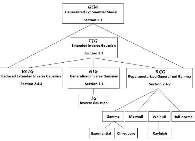
1.1 Relationships between the models introduced in this thesis . . . 6

2.1 The effect ofξon theGEM . . . 8

2.2 The effect ofξon theGEM(Continued) . . . 8

2.3 The effect ofδon theGEM . . . 9

2.4 The effect ofνon theGEM . . . 9

2.5 The effect ofτon theGEM . . . 10

2.6 The effect ofρon theGEM. . . 10

2.7 OriginalGEM superimposed on the proxy model (red line) expanded with 3 terms around 2/3. . . 22

2.8 OriginalGEM superimposed on the proxy model (red line) expanded with 4 terms around 2/3. . . 22

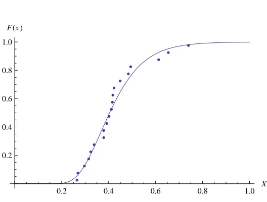
2.9 The empirical CDF and the fitted Weibull CDF for the flood data set. . . 29

2.10 The empirical CDF and the fitted lognormal CDF for the flood data set.. . . 30

2.11 The empirical CDF and the fitted generalized inverse Gaussian CDF for the Flood data set. . . 30

2.12 The empirical CDF and the fitted five parameterGEMCDF for the Flood data set. . . 31

2.13 The empirical CDF and the fitted inverse Gaussian CDF using the method of moments for the Flood data set . . . 31

2.14 The empirical CDF and the fitted five parameterGEMCDF using the method of moments for the Flood data set. . . 33

2.15 The empirical CDF and the fitted inverse Gaussian CDF using the method of moments for the Flood Data set . . . 33

2.16 The empirical CDF and the fitted five parameter GEM using the method of moments for the Flood Data set . . . 35

2.17 The empirical CDF and the fitted proxyGIGCDF using the maximum likeli-hood method for the Flood data set . . . 35

2.18 The empirical CDF and the fitted proxyGEMCDF using the maximum likeli-hood method for the Flood data set . . . 37

3.1 Effect ofξon theEIGdistribution.. . . 40

3.2 Effects ofδ(left panel) andν(right panel) on theEIGmodel. . . 41

3.3 Effect ofτon theEIGdistribution.. . . 41

3.4 Effects ofξ(left panel) andδ(right panel) on theREIGmodel.. . . 42

3.5 Effect ofτon theREIGdistribution. . . 42

(9)

3.7 CDF (solid line) and empirical CDF (dots) for the flood data set. Left panel:

EIG; Right panel:REIG. . . 49

3.8 CDF (solid line) and empirical CDF (dots) for the snowfall data set. Left panel: Lognormal; Right panel: GIG. . . 51

3.9 CDF (solid line) and empirical CDF (dots) for the snowfall data set. Left panel: RGG; Right panel:EIG. . . 51

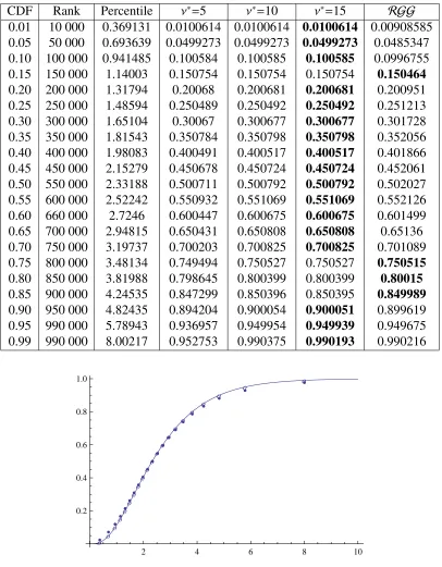
4.1 The empirical CDF (dots), the CDF resulting from Equation (4.22) (circles) and the fittedRGGCDF (solid line) k=2 . . . 60

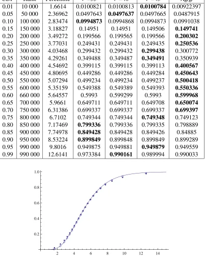
4.2 The empirical CDF (dots), the CDF resulting from Equation (4.22) (circles) and the fittedRGGCDF (solid line) for k=4 . . . 61

4.3 The empirical CDF (dots), the CDF resulting from Equation (4.22) (circles) and the fittedRGGCDF (solid line) for k=5 . . . 62

5.1 Plot of Canadian quinquennial mortality rates (times 1000) in 2006 for ages 15 and over . . . 65

5.2 Interpolation function (third degree splines) for the Canadian quinquennial mortality rates data set . . . 65

5.3 Derivative of the interpolating function for the Canadian quinquennial mortal-ity rates . . . 66

5.4 Density function corresponding to Canadian quinquennial mortality rates ob-tained after applying numerical differentiation, reflection and normalization . . 67

5.5 Original and fitted mortality rates using theRGGmodel . . . 68

5.6 Original and fitted mortality rates using theGEM . . . 68

5.7 Fitted function superimposed on the mortality rates . . . 68

6.1 Bivariate histogram of the flood data. . . 72

6.2 EIGunivariate density estimate for the waiting time in the bivariate flood data . 72 6.3 RGGunivariate density estimate for the waiting time variable in the bivariate flood data . . . 72

6.4 The empirical CDF and the fittedEIGCDF for the flood peaks variable in the bivariate flood data . . . 73

6.5 The empirical CDF and the fittedRGGCDF for the flood peaks variable in the bivariate flood data . . . 73

6.6 The empirical CDF and the fitted EIG CDF for the volume variable in the bivariate flood data . . . 74

6.7 The empirical CDF and the fittedEIGCDF for the flood peaks variable in the bivariate flood data . . . 74

6.8 IGbivariate density estimate for the bivariate flood data . . . 75

6.9 EIGbivariate density estimate for the bivariate flood data . . . 75

6.10 Bivariate histogram for the Old Faithful data . . . 75

6.11 RGGbivariate density estimate for the Old Faithful data. . . 77

6.12 EIGbivariate density estimate for the Old Faithful data . . . 77

(10)

List of Tables

2.1 Maximum Flood Levels . . . 29

2.2 Estimates of the Parameters and Goodness-of-Fit Statistics for Maximum Flood Levels . . . 32 2.3 The Bufffalo Snow Data Set . . . 32 2.4 Estimates of the Parameters and Goodness-of-Fit Statistics for the Snowfall

Data Set . . . 34 2.5 The Repair Time Data Set . . . 34 2.6 Estimates of the Parameters and Goodness-of-Fit Statistics for the Repair Data

Set . . . 36 2.7 Estimates of the Parameters and Goodness-of-Fit Statistics for the Maximum

Flood data using the Moment Method . . . 36 2.8 Estimates of Parameters and Goodness-of-Fit Statistics for the Three Data Sets

Using a Proxy Distribution with 7 Terms . . . 37 2.9 Estimates of Parameters for Various Data Sets Using NIntegrate for

Determin-ing the NormalizDetermin-ing Constant . . . 37 2.10 Goodness-of-Fit Statistics for Various Data Sets Using NIntegrate for

Deter-mining the Normalizing Constant . . . 37 2.11 Estimates of the Parameters for Various Data Sets Using NIntegrate for

Deter-mining the Normalizing Constant (5 Parameters) . . . 38 2.12 Goodness-of-Fit Statistics for Various Data Sets Using NIntegrate for

Deter-mining the Normalizing Constant (5 Parameters) . . . 38 2.13 Loglikelihood Function and BIC for Various Data Sets . . . 38

3.1 Maximum Flood Level Data . . . 48 3.2 Parameter Estimates and A2

0&W02for the Flood Data . . . 48

3.3 The Snowfall Precipitation Data . . . 50 3.4 Parameter Estimates and A2

0&W02for the Snowfall Data . . . 50

3.5 The Breaking Stress Data . . . 51 3.6 Parameter Estimates and A2

0&W02for the Breaking Stress Data . . . 52

3.7 Parameter Estimates and A2

0&W02for the Breaking Stress Data . . . 52

4.1 Parameter Values of the Three Linear Combinations . . . 59 4.2 CDF Approximations for a Linear Combination of Two Variables, (k=2), Using

theRGGModel and the Truncated Density (4.23) . . . 60 4.3 CDF Approximations for a Linear Combination of Four Variables, (k=4),

Us-ing theRGGModel and the Truncated Density (4.23) . . . 61

(11)

5.1 Canadian Quinquennial Mortality Rates (times 1000) in 2006 for Ages 15 and

Over . . . 66

5.2 Parameter Estimates and ASD’s for the Canadian Quinquennial Mortality Rates 67 5.3 Mortality Rates for Females for ages 8-102 . . . 69

5.4 Parameter Estimates and ASD’s for the Female Mortality Rates . . . 69

6.1 The Flood Data Set . . . 71

6.2 Parameter Estimates for the Bivariate Flood Data . . . 73

6.3 A2 0&W02for the Bivariate Flood Data . . . 74

6.4 The Old Faithful Data Set . . . 76

6.5 A2 0&W02for the Old Faithful Data . . . 77

(12)

Chapter 1 Introduction

1.1 Introduction

As pointed out in Balakrishnan and Basu (1995), the gamma family of distributions was discussed by Karl Pearson as early as 1895. However, it took another 35 years for the exponen-tial distribution, which is a special case, to appear on its own: While discussing the sampling distribution of the standard deviation, Kondo (1930) referred to the exponential distribution as Pearson’s Type X distribution. Applications of the exponential distribution in actuarial, bio-logical and engineering problems were respectively proposed by Steffensen (1930), Teissier (1934) and Weibull (1939).

Both the shape and scale parameters of the gamma distribution can have non-integer val-ues. The gamma distribution has two types of applications. First, applications based on in-tervals between events; in this form, examples of its use include queuing models, the flow of items through manufacturing and distribution processes, the load on web servers, and the many and varied forms of telecom exchange. The other type of applications takes advantage of the gamma distribution moderately skewed profile; accordingly, this model can be utilized in sev-eral disciplines such as climatology where it is a workable model for rainfall and in actuarial mathematics where it has been used for modeling insurance claims, the size of loan defaults, and for determining the probability of ruin and the value at risk.

An extension of the exponential distribution referred to as the Weibull distribution was proposed by Weibull (1951). The exponential distribution is a special case wherein the shape parameter equals one. As explained in Lai et al. (2006), the Weibull distribution has many applications in survival analysis and reliability engineering. Several applications in industrial quality control are also discussed in Berrettoni (1964).

A generalized exponential model (GEM) distribution is being introduced in Chapter 2. Its density function is given by

fA(x)= c xξ+δe−νx

δ

e−τx−ρ

IR+(x), (1.1)

whereIB(x) denotes the indicator function of the set B, R+is the set of real positive numbers

and c is a normalizing constant. The parameters ν, δ, τ and ρ are assumed to be positive

(13)

whileξcan be any real number. The extension proposed in this thesis is more general than the generalized inverse Gaussian model introduced by Jørgensen (1982).

Numerous distributions are special cases of the proposed generalized exponential model. For instance, the following distributions arise as special cases of (1.1) whereinτ= 0:

(i) The gamma distribution — denotedΓ(α, β)— with density function

f(x)= x

α−1_exp(₋_x_/β₎

βα_Γ(_θ₎ IR+(x), α, β >0, is obtained by lettingξ =α−2, ν= 1/β,andδ= 1.

(ii) The Weibull distribution with density function

f(x)=θ φxφ−1_exp(₋_θ_xφ₎_I

R+(x), is obtained by lettingξ =−1, ν=θandδ= φ.

(iii) The Maxwell distribution with density function

f(x)= 4x

2_exp(₋_x2_/θ2₎

θ3√_π IR+(x),

is obtained by lettingξ =0, ν= 1/θ2_and_δ ₌₂_.

(iv) The half-normal distribution with density function

f(x)= 2 exp(−x

2_/₍₂_θ2₎₎

θ√2π IR+(x), θ > 0,

is obtained by lettingξ =−2, ν=1/2θ2_and_δ₌₂_.

(v) The exponential distribution with density function

f(x)= exp(−x/κ)

κ IR+(x), φ > 0,

is obtained by lettingξ =−1, ν=1/κandδ= 1.

(vi) The chi-square distribution with density function

f(x)= xν/2−1exp(−x/2)

2ν/2_Γ(_ν/₂₎ IR+(x), ν >0,

is obtained by lettingξ =ν/2−2, ν=1/2 andδ= 1.

(vii) The Rayleigh distribution with density function

f(x)= xexp(−x

2_/₍₂_a2₎₎

(14)

1.1. I 3

is obtained by lettingξ =−1, ν=1/(2a2_{) and}_δ ₌₂_.

The density function of the inverse Gaussian distribution with real parameters µ ∈ Rand

λ >0 has the following form:

f(x)= r

λ

2πx3 exp(−λ(x−µ)

2_/₍₂_x_µ2₎₎_I

R+(x). (1.2)

This density function is a particular case of the density function given in (1.1) withξ = −5/2, ν = λ/(2µ2₎_{, δ} ₌ ₁_{, τ} ₌ _λ/_{2 and}_ρ ₌ ₁_. _{It should be note that several other parameterizations}

are possible and that, in this case,τ,0.

Jørgensen (1982) proposed the so-called Generalized Inverse Gaussian (GIG) distribution whose density function is given by

f(x)= (φ/θ)λ/2 2Kλ(

√ θ φ) x

λ−1_exp(₋₍_θ_x−1₊_φ_x₎_/₂₎_I

R+(x), (1.3)

whereKλ(·) denotes a modified Bessel function of the second kind. The density function given in (1.3) is a special case of the five-parameter exponential distribution withξ= λ−2, ν= φ/2, δ= 1, τ= θ/2,andρ=1.

One can also obtain special cases from the symmetrized form of (1.1), that is,

fS(x)=

fA(|x|)

2 IR(x). For instance, the normal distribution with density function

f(x)= 1

σ√2π exp(−x

2_/₍₂_σ2₎₎_I

R(x), σ >0,

is obtained by lettingτ = 0, ξ = −2, ν = 1/2σ2_, _and_δ ₌ ₂_. _{The lognormal(}_{µ, σ}_{) distribution}

is then obtained via the transformation y = ex_{. Another example is the double-exponential}

distribution with density function

f(x)= θ

2 exp(−θ|x|)IR(x), θ >0,

which turns out to be a particular case of fS(x) whereinτ =0,ξ= −1, ν= θ,andδ =1.

Moreover, a location parameterm can readily be incorporated in the density functions by replacingxwithx−m.

The inverse Mellin transform technique will be used to determine the moments and the normalizing constant of the proposed distribution and other sub-class distributions. A brief introduction to this transform and its inverse is hereby provided.

(15)

Mf(s) =

∞

0 xs−1f(x) dx is the Mellin transform of f(x). Whenever f(x) is continuous, the

corresponding inverse Mellin transform is

f(x)= 1 2πi

Z _c₊_i_∞

c−i∞

x−sMf(s) ds (1.4)

which, together withMf(s),constitute a transform pair. The path of integration in the complex

plane is called the Bromwich path. Equation (1.4) determines f(x) uniquely if the Mellin transform is an analytic function of the complex variablesforc1≤ <(s)=c≤c2wherec1and

c2are real numbers and<(s) denotes the real part ofs.In the case of a continuous nonnegative

random variable whose density function is f(x), the Mellin transform is its moment of order (s−1) and the inverse Mellin transform yields f(x).

Letting

Mf(s)=

n Q_m

j=1Γ(bj+Bjs)

o nQ_n

i=1Γ(1−ai−Ais)

o

nQ_q

j=m+1Γ(1−bj−Bjs)

o nQ_p

i=n+1Γ(ai +Ais)

o ≡ h(s) (1.5)

where an empty product (for example when n = p) is interpreted as unity and m,n,p,q are nonnegative integers such that 0 ≤ n ≤ p, 1 ≤ m ≤ q, Ai, i = 1, . . . ,p, Bj, j = 1, . . . ,q,

are positive numbers andai, i = 1, . . . ,p, bj, j = 1, . . . ,q,are complex numbers such that

−Ai(bj+ν), Bj(1−ai+λ) forν, λ =0,1,2, . . . , j=1, . . . ,m,andi=1, . . . ,n,theH–function

can be defined as follows in terms of the inverse Mellin transform ofMf(s):

f(x)=Hm,n p,q x

(a1,A1), . . . ,(ap,Ap)

(b1,B1), . . . ,(bq,Bq)

!

= 1

2πi

Z _c₊_i_∞

c−i∞

h(s)x−s_d_s _(1.6)

whereh(s) is as defined in (1.5) and the Bromwich path (c−i∞, c+i∞) separates the points

s = −(bj +ν)/Bj, j = 1, . . . ,m, ν = 0,1,2, . . . , which are the poles ofΓ(bj + Bjs), j = 1, . . . ,m, from the pointss=(1−ai+λ)/Ai, i=1, . . . ,n, λ=0,1,2, . . . ,which are the poles

ofΓ(1−ai−Ais), i= 1, . . . ,n.Thus, one must have

Max

1≤ j≤m<{−bj/Bj}<c< Min1≤i≤ n<{(1−ai)/Ai}. (1.7)

If, for certain parameter values, anH–function remains positive on the entire domain, then whenever the existence conditions are satisfied, a probability density function can be generated by normalizing it. For example, the Weibull, chi-square, half–normal and F distributions can all be expressed in terms ofH-functions. For the main properties of theH–function as well as its applicability to various disciplines, the reader is referred to Mathai and Saxena (1978) and Mathai (1993).

When Ai = Bj = 1 fori = 1, . . . ,pand j = 1, . . . ,q, theH–function reduces to Meijer’s G–function, that is,

Gm,n p,q x

a1, . . . ,ap

b1, . . . ,bq

!

≡ Hm,n p,q x

(a1,1), . . . ,(ap,1)

(b1,1), . . . ,(bq,1)

!

(16)

1.1. I 5

Moreover, theG–function satisfies the following identity:

Gm_p_,,_qn xa1, . . . ,ap b1, . . . ,bq

!

=Gn_q,_,m_p 1

x

1−b1, . . . ,1−bq

1−a1, . . . ,1−ap

!

. (1.9)

Chapter 3 introduces an extension of the generalized inverse Gaussian distribution, which was extensively discussed in Jørgensen (1982). A related model is proposed as well. The effects of the parameters on these models are illustrated graphically. These distributions are fitted to several data sets, the goodness of fit being determined by means of the Anderson-Darling and the Cram´er-von Mises statistics.

It is explained in Chapter 4 that quadratic forms in central normal vectors whose density function is often approximated in terms of exponential-type densities, can be reduced to linear combinations of chi-square random variables. We are making use of the inverse Mellin trans-form technique to obtain a multiple series representation of the density function of such linear combinations. The accuracy of the truncated form of density function is compared in several examples to that obtained from the reparameterized generalized gamma distribution, which is a particular case of the generalized exponential model.

The hazard and the mean residual life functions are determined for some of the proposed distributions in Chapter 5. Two actuarial data sets are fitted with the generalized exponential model. This is achieved by introducing a method whereby regression problems of this type can be converted into density estimation problems.

In the final chapter, a technique is proposed for modelling bivariate data. First the data is normalized and shifted to ensure that the variables be uncorrelated and that their support be essentially positive. Then, each variable is fitted individually with some of the proposed models, after which the inverse transformation is applied to the resulting bivariate density. Histograms of the data sets and plots of the final bivariate density estimates are included for comparison purposes. This approach could be extended to multivariate data sets.

The proposed extended and generalized exponential distributions should provide more ac-curate univariate or multivariate models in connection with the host of applications that rely on exponential-type distributions, which arise in numerous fields of scientific investigations. For convenience theMathematicacodes utilized in connection with the main applications pre-sented in this thesis are included in the Appendix.

(17)

Figure 1.1: Relations between different models introduced in the thesis

Printed by Mathematica for Students

(18)

Chapter 2 The Generalized Exponential Model

2.1 Introduction

This chapter explores the properties of the proposed probability distribution called the Gen-eralized Exponential Model (GEM) whose associated density function is given by

fA(x)= c xξ+δe−νx

δ

e−τx−ρ

IR+(x), (2.1)

whereIB(x) denotes the indicator function of the set B, R+is the set of real positive numbers

andcis a normalizing constant. The parametersν, δ, τandρ,are assumed to be positive while

ξ can be any real number. For simplification purposes, at times,δand ρwill be expressed as fractions, that is,δ= a/dandρ=w/rwherea, d, w,andrare positive integers.

Section 2.2 shows graphically how theGEMis affected by its five parameters and Section 2.3 presents the derivation of theh-moment of theGEMdistribution. Some statistical functions such as the mean, certain central moments, the cumulative distribution function, the mode and the moment generating function of the GEM and some of its sub-class models are given in Section 2.4. In addition, a probability distribution model which approximates the GEM is introduced in the same section. This distribution is referred to as the proxy distribution and is computationally more convenient than the GEM. Section 2.5 gives an introduction on the parameter estimation methods that are employed in this thesis, while Section 2.6 shows that products and ratios of certain exponential-type distributions can be expressed in terms of the moments of the proposed five-parameter exponential-type distribution, which in turn can be expressed in terms of generalized hypergeometric functions. In section 2.7 three data sets, namely the maximum flood levels, snowfall precipitation and repair time data sets, are fitted to theGEMand its proxy distribution.

2.2 Parameter E

ff

ects

This section illustrates graphically how the generalized exponential model specified by Equation (2.1) is affected by its parameters. Figure 2.1 and 2.2 show that ξ works as a scale

(19)

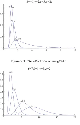
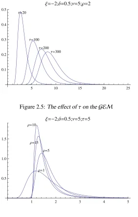
and shift parameter. Figure 2.3- 2.6 shows the scale effect ofδ, νandρand the shift effect ofτ

on the proposed distribution.

2 4 6 8 10 12 14

0.2 0.4 0.6 0.8 1.0 1.2 1.4

∆=1;Ν=2;Τ=3;Ρ=2

Ξ=-2 Ξ=-5

Ξ=1

Ξ=7

Figure 2.1:The effect ofξon theGEM

20 40 60 80

0.05 0.10 0.15

∆=1;Ν=2;Τ=3;Ρ=2

Ξ=20

Ξ=40

Ξ=60 Ξ=80

Ξ=100

(20)

2.2. PE 9

2 4 6 8 10

0.5 1.0 1.5

Ξ=-1,Ν=2,Τ=3,Ρ=2;

∆=32 ∆=52

∆=12

Figure 2.3:The effect ofδon theGEM

5 10 15 20

0.1 0.2 0.3 0.4 0.5 0.6 0.7

Ξ=7;∆=1;Τ=3;Ρ=2

Ν=3 Ν=5

Ν=1 Ν=1.5

(21)

5 10 15 20 25 0.1

0.2 0.3 0.4 0.5

Ξ=-2;∆=0.5;Ν=5;Ρ=2

Τ=20

Τ=100

Τ=200 Τ=300

Figure 2.5:The effect ofτon theGEM

1 2 3 4 5

0.5 1.0 1.5

Ξ=-2;∆=0.5;Ν=5;Τ=5

Ρ=1 Ρ=5 Ρ=10

Ρ=15

Figure 2.6:The effect ofρon theGEM

2.3 Moments of the Generalized Exponential Model

Consider a random variable X whose density function is given by (2.1). In order to deter-mine itshth_{moment, one has to evaluate the integral,}

c

Z _∞

0

xξ+δ+he−νxδe−τx−ρdx. (2.2)

(22)

2.3. M  GEM 11

integral is then obtained. So, let X1 and X2 be independently distributed random variables

whose density functions are

g1(x1)=c1x1e−νx

δ

1 I_R+(x₁) and

h1(x2)= c2e−x

ρ

2 I_R+(x₂), whose (t−1)th_{moments are respectively}

c1

ν−t+ δ Γ t+ δ δ and c2

Γt

ρ

ρ ,

c1andc2being normalizing constants. Thus the (t−1)thmoment ofU =X1X2can be expressed

as

k(t)=c1c2

ν−t+

δ Γ

t+ δ

Γt

ρ

δ ρ .

The density function of U = X1X2 obtained by taking the inverse Mellin transform of

k(t),that is,

1 2πi

Z

C

u−t_k₍_t_{) d}_t_,

where i = √−1 andCis a contour of integration which encompasses the poles of Γt

ρ

and

Γ

δ+ δt

,is

c1c2ν−

δ δ ρ

1 2πi

Z

C

uν1δ

−t Γ _t₊ δ Γ t ρ ! dt (2.3)

= c1c2ν−

δ δ ρ H

2,0 0,2 uν

1

δ

{(0,1/ρ),( δ, 1δ)}

!

, (2.4)

where theH-function is as defined in the Introduction.

When δ and ρ are rational numbers such that δ = a/d and ρ = w/r, where a, d, w, r

are positive integers, one can express the integral in (2.3) as a Meijer’sG-function by letting

(23)

Γ(r+q s)= (2π)1−2qqr+q s−12 q−1

Y

k=0

Γk+r

q + s

. (2.5)

The density function ofUis then

c1c2d rν−

d

a (2π)−r a2−d w2 +1(d w)da−12(r a)−1/2

×

Z

C0

ua w_νwd

(r a)r a₍_{d w}₎d w

−zQ_{d w}₋₁ k=0 Γ

z+ k+da

d w

Q_{r a}₋₁

k=0 Γ

k r a+z

2πi dz, (2.6)

that is,

c1c2d rν−

d

a (2π)−r a2−d w2 +1(d w)da−12(r a)−1/2

× Gd w₀_,_{d w}+r a₊_{r a},0 u

a w_νw d

(r a)r a₍_{d w}₎d w

k+d

a

d w ,k= 0, ...,d w−1;r ak ,k=0, ...,r a−1

!

(2.7)

Now, considering the transformation U = X1X2 and W = X1, it is seen that the density

function ofUis also given by

r(u) = Z _∞

0

1

w g1(w)h1(u/w) dw

= c1c2

Z _∞

0

1

wv

_e−νwδ

e−(u/w)ρ

dw, (2.8)

and letting = ξ +δ+h+1 and u = τ1/ρ_{, the integral in (2.8) is seen to coincide with that} appearing in Equation (2.2). Thus thehth_{moment of}_X_is

mX(h)= cν

−ξ+δ+_δh+1

δ ρ H

2,0

0,2 τ1/ρν1/δ

{(0,1/ρ),(ξ+δ+_δh+1,1

δ)} !

(2.9)

or, in light of Equation (2.7),

m(_XR)(h)=c d rν−d(ξ+_ah+1)−1₍₂_π₎−r a

2−d w2 +1(d w)

d(ξ+h+1)

a +12(r a)−1/2

×Gd w₀_,_{d w}+r a₊_{r a},0 τ

r a_νwd

(r a)r a₍_{d w}₎d w

k+

d(ξ+h+1)

a +1

d w ,k= 0, ...,d w−1; k

r a,k =0, ...,r a−1

!

(2.10)

whereρandδare rational numbers such that

(24)

2.3. M  GEM 13

and

ρ=w/r.

Now assuming thatδ = ρand lettingw= t/δ, = ξ+δ+h+1 andu= τ1/ρ _{in the integral} in (2.3), one obtains thehth_{moment of}_X _as

m(_XE)(h)=cν−

h+ξ+1

δ −1 δ G

2,0 0,2 ν τ

0,ξ+h_δ+1 +1 !

,

which can also be expressed in terms of a Bessel function of the second kind as

2ν−h+ξ+δδ+1

ν1δτ1δ

h+ξ+δ+1 2δ

Kh+ξ+δ+1

δ

2pν1δτ1δ

δ .

where Kλ(·) is a modified Bessel function of the second type that has the following integral representation:

Kλ(η)= 1 2

Z _∞

0

xλ−1e12η(x+x−1)dx.

Incidentally, Kλ(·) is a built-in function in the symbolic computing package Mathematica. As explained in Abramowitz and Stegun (1972), the modified Bessel functions of the first and second types, namelyIλ(w) andKλ(w),are the two linearly independent solutions of the differ-ential equationw2 d2y

dw2 + w

dy

dw −(w2 + λ2)y= 0.

Since the null moments are equal to one, the normalizing constantcis seen to be the inverse of the moment expressionsmX(h),m(_XR)(h), andm(_XE)(h), whereinhis set equal to zero andcis omitted. When there are no restrictions onδandρ,the normalizing constant in (2.1) is

c= δ ρ ν

ξ+1

δ +1 H₀2_,,₂0 τ1ρν1δ

{(0,1/ρ),(ξ+_δ1 +1, 1

δ)}

!, (2.11)

whenδandρare rational numbers, the normalizing constant will be

c(R)=

νd(ξa+1)+1₍₂_π₎r a2+d w2 −1₍_{d w}₎−d(ξa+1)−12₍_{r a}₎1/2 d r

Gd w₀_,_{d w}+r a₊_{r a},0 τr a_νwd

(r a)r a₍_{d w}₎d w

k+d(ξ_a+1)+1

d w ,k=0,...,d w−1;r ak,k=0,...,r a−1

!,

(2.12)

and whenδ=ρ, one has

c(E) = δ ν

ξ+1

δ +1 G2₀,_,0₂ ν τ

0, ξ+δ1+1 !

= δ ν

ξ+δ+1

δ

2 (ντ)ξ+2δδ+1 K_ξ₊_δ₊₁ δ

(25)

2.4 Some Statistical Functions

2.4.1 Generalized Exponential Model (

GEM

)

Let X be a random variable whose p.d.f is specified by (2.1), then some related statistical functions of theGEMare obtained.

(i) The expectation ofXis

E(X) = (dw

ν )d/aG

d w+r a,0 0,d w+r a τ

r a_νwd

(r a)r a₍_{d w}₎d w

k+d(

a d+ξ+2)

a

dw ,k=0,...,dw−1,rak,k=0,...,ra−1

!

Gd w₀_,_{d w}+r a₊_{r a},0 τr a_νd w

(r a)r a₍_{d w}₎d w

k+d(

a d+ξ+1)

a

dw ,k=0,...,dw−1,rak,k=0,...,ra−1

! (2.14)

(ii) The variance ofX is

Var(X) = (dw

ν )

2d

aGd w+r a,0

0,d w+r a τ

r a_νd w

(r a)r a₍_{d w}₎d w

k+d(

a d+ξ+3)

a

dw ,k=0,...,dw−1,rak,k=0,...,ra−1

!

(r a)r a₍_{d w}₎d w

k+d(

a d+ξ+1)

a

dw ,k=0,...,dw−1,rak,k=0,...,ra−1

!

−

(dw

ν )

2d

a Gd w+r a,0

0,d w+r a τ

r a_νd w

(r a)r a₍_{d w}₎d w

k+d(

a d+ξ+2)

a

dw ,k=0,...,dw−1,rak,k=0,...,ra−1

!2

(r a)r a₍_{d w}₎d w

k+d(

a d+ξ+1)

a

dw ,k=0,...,dw−1,rak,k=0,...,ra−1

(26)

2.4. SSF 15

(iii) The skewness ofXis

s(X) = (

(dw)2adν−3ad

×

3νdaGd w+r a,0

0,d w+r a

τr a_νd w

(r a)r a₍_{d w}₎d w

k+d(

a d+ξ+2)

a

dw ,k=0,...,dw−1,rak,k=0,...,ra−1

2

+

Gd w+r a,0 0,d w+r a

τr a_νd w

(r a)r a₍_{d w}₎d w

k+d(

a d+ξ+4)

a

dw ,k=0,...,dw−1,rak,k=0,...,ra−1

× Gd w₀_,_{d w}+r a₊_{r a},0

τr a_νd w

(r a)r a₍_{d w}₎d w

k+d(

a d+ξ+1)

a

dw ,k=0,...,dw−1,rak,k=0,...,ra−1

−3Gd w₀_,_{d w}+r a₊_{r a},0

τr a_νd w

(r a)r a₍_{d w}₎d w

k+d(

a d+ξ+2)

a

dw ,k=0,...,dw−1,rak,k=0,...,ra−1

×(dw)daGd w+r a,0

0,d w+r a

τr a_νd w

(r a)r a₍_{d w}₎d w

k+d(

a d+ξ+3)

a

dw ,k=0,...,dw−1,rak,k=0,...,ra−1

)

÷

(

Gd w₀_,_{d w}+r a₊_{r a},0

τr a_νd w

(r a)r a₍_{d w}₎d w

k+d(

a d+ξ+1)

a

dw ,k=0,...,dw−1,rak,k=0,...,ra−1

2 × ( (dw ν ) 2d a

Gd w₀_,_{d w}+r a₊_{r a},0

τr a_νd w

(r a)r a₍_{d w}₎d w

k+d(

a d+ξ+3)

a

dw ,k=0,...,dw−1,rak,k=0,...,ra−1

× Gd w₀_,_{d w}+r a₊_{r a},0

τr a_νd w

(r a)r a₍_{d w}₎d w

k+d(

a d+ξ+1)

a

dw ,k=0,...,dw−1,rak,k=0,...,ra−1

− Gd w₀_,_{d w}+r a₊_{r a},0

τr a_νd w

(r a)r a₍_{d w}₎d w

k+d(

a d+ξ+2)

a

dw ,k=0,...,dw−1,rak,k=0,...,ra−1

2

÷ Gd w₀_,_{d w}+r a₊_{r a},0

τr a_νd w

(r a)r a₍_{d w}₎d w

k+d(

a d+ξ+1)

a

dw ,k=0,...,dw−1,rak,k=0,...,ra−1

2)3/2)

(2.16)

(iv) The kurtosis ofX is

k(X) = ( dw ν 4d a × (

−4Gd w₀_,_{d w}+r a₊_{r a},0

τr a_νd w

(r a)r a₍_{d w}₎d w

k+d(

a d+ξ+2)

a

dw ,k=0,...,dw−1,rak,k=0,...,ra−1

4

×8Gd w₀_,_{d w}+r a₊_{r a},0

τr a_νd w

(r a)r a₍_{d w}₎d w

k+d(

a d+ξ+3)

a

dw ,k=0,...,dw−1,rak,k=0,...,ra−1

× Gd w₀_,_{d w}+r a₊_{r a},0

τr a_νd w

(r a)r a₍_{d w}₎d w

k+d(

a d+ξ+1)

a

dw ,k=0,...,dw−1,rak,k=0,...,ra−1

(27)

× Gd w₀_,_{d w}+r a₊_{r a},0

τr a_νd w

(r a)r a₍_{d w}₎d w

k+d(

a d+ξ+2)

a

dw ,k=0,...,dw−1,rak,k=0,...,ra−1

2

+Gd w₀_,_{d w}+r a₊_{r a},0

τr a_νd w

(r a)r a₍_{d w}₎d w

k+d(

a d+ξ+5)

a

dw ,k=0,...,dw−1,rak,k=0,...,ra−1

× Gd w+r a,0 0,d w+r a

τr a_νd w

(r a)r a₍_{d w}₎d w

k+d(

a d+ξ+1)

a

dw ,k=0,...,dw−1,rak,k=0,...,ra−1

3

−

(

Gd w+r a,0 0,d w+r a

τr a_νd w

(r a)r a₍_{d w}₎d w

k+d(

a d+ξ+3)

a

dw ,k=0,...,dw−1,rak,k=0,...,ra−1

2

+4Gd w₀_,_{d w}+r a₊_{r a},0

τr a_νd w

(r a)r a₍_{d w}₎d w

k+d(

a d+ξ+2)

a

dw ,k=0,...,dw−1,rak,k=0,...,ra−1

× Gd w₀_,_{d w}+r a₊_{r a},0

τr a_νd w

(r a)r a₍_{d w}₎d w

k+d(

a d+ξ+4)

a

dw ,k=0,...,dw−1,rak,k=0,...,ra−1

)

× Gd w₀_,_{d w}+r a₊_{r a},0

τr a_νd w

(r a)r a₍_{d w}₎d w

k+d(

a d+ξ+1)

a

dw ,k=0,...,dw−1,rak,k=0,...,ra−1

2

+Gd w₀_,_{d w}+r a₊_{r a},0

τr a_νd w

(r a)r a₍_{d w}₎d w

k+d(

a d+ξ+5)

a

dw ,k=0,...,dw−1,rak,k=0,...,ra−1

× Gd w₀_,_{d w}+r a₊_{r a},0

τr a_νd w

(r a)r a₍_{d w}₎d w

k+d(

a d+ξ+1)

a

dw ,k=0,...,dw−1,rak,k=0,...,ra−1

3))

× Gd w₀_,_{d w}+r a₊_{r a},0

τr a_νd w

(r a)r a₍_{d w}₎d w

k+d(

a d+ξ+1)

a

dw ,k=0,...,dw−1,rak,k=0,...,ra−1

4

(v) The mode of f(x) satisfies the following equation:

x=ρ τx−ρ₋_{δ ν}_xδ₊_δ₊_ξ.

It is obtained by equating the derivative of the probability density function ofX given in (2.1) to zero.

2.4.2 Reparameterized Generalized Gamma (

RGG

) Model

TheRGGmodel is a reduced form of theGEMmodel, which is obtained by omittinge−τx−ρ

(or equivalently by lettingτ =0) in the density function (2.1), which yields

f(x)= δν

δ+ξ δ

Γ δ+_δξx

ξ+δ−1_e−νxδ

IR+(x), (2.17)

whereδ+ξ >0.This density function is in fact a Reparameterized Generalized Gamma (RGG) density function, which is obtained by lettingβ= δ, θ=ν−1/β _and_k ₌ δ+ξ+1

δ in the generalized gamma density,

g1(x)=

β θkβ_Γ(_k₎ x

kβ−1_e−(x

(28)

2.4. SSF 17

For specific distributional results in connection with the generalized gamma distribution, the reader is referred to Johnsonet al.(1994).

LetXbe anRGGrandom variable. Then, (i) Thekth_{moment of}_X_is

E(Xk₎₌ ν−

k

δΓ k+δ+ξ

δ

Γ δ+_δξ ; (2.19)

(ii) The expectation ofXis

E(X)= ν

−1/δ_Γ δ+ξ+1

δ

Γ δ+_δξ ; (2.20)

(iii) The variance ofX is

Var(X)= ν

−2/δ_Γ δ+ξ+2

δ

Γ δ+_δξ −

ν−2/δ_Γ δ+ξ+1

δ ₂

(29)

2.4.3 Reduced Extended Inverse Gaussian (

REIG

) Model

The REIGmodel is a reduced form ofGEM model which is obtained by omittinge−νxδ

(or equivalently by lettingν = 0) in the density function (2.1). It is also a reduced form of the extended inverse Gaussian distribution which is defined in Section 3.1, hence the name. Thus, the density function ofREIGmodel is given by

f(x)= ρ τ

−ξ+ρ_ρ+1

Γ − ξ+ρ_ρ+1 x

ξ+ρ_e−τx−ρ

IR+(x), ξ+ρ+1< 0, (2.26)

LetXbe anREIGrandom variable. Then, (i) Thekth_{moment of}_X_is

τk/ρ_Γ ₋ k+ξ+ρ+1

ρ

Γ − ξ+ρ_ρ+1 ; (2.27)

(ii) The expectation ofXis

E(X)= τ

1

ρΓ − ξ+ρ+2

ρ

Γ − ξ+ρ_ρ+1 ; (2.28)

(iii) The variance ofX is

Var(X)= τ

2/ρ_Γ ₋ ξ+ρ+3

ρ

Γ − ξ+ρ_ρ+1 −

τ2/ρ_Γ ₋ ξ+ρ+2

ρ 2

Γ − ξ+ρ_ρ+12 ; (2.29)

(iv) The skewness ofXis

s(X)= 2Γ −

ξ+ρ+2

ρ

3

−3Γ −ξ+ρρ+1

Γ −ξ+ρρ+3

Γ −ξ+ρρ+2

+Γ −ξ+ρρ+1

2

Γ−ξ+ρρ+4

Γ − ξ+ρ_ρ+1Γ − ξ+_ρρ+3−Γ − ξ+ρ_ρ+22

3/2 ; (2.30)

(v) The kurtosis ofXis

k(X) = 6τ

4/ρ_Γ₋ξ+ρ+2

ρ ₂

Γ−ξ+ρ_ρ+3

Γ−ξ+ρ_ρ+13

− 4τ

4/ρ_Γ₋ξ+ρ+2

ρ

Γ−ξ+ρ_ρ+4

Γ−ξ+ρ_ρ+12

−

   

τ2/ρ_Γ₋ξ+ρ+3

ρ

Γ−ξ+ρ_ρ+1 −

τ2/ρ_Γ₋ξ+ρ+2

ρ 2

Γ−ξ+ρ_ρ+12

   

2

−3τ

4/ρ_Γ₋ξ+ρ+2

ρ ₄

Γ−ξ+ρ_ρ+14

+ τ

4/ρ_Γ₋ξ+ρ+5

ρ

(30)

2.4. SSF 19

(vi) The mode ofREIGmodel is

x= e−iρπρ1ρ(ξ+ρ)−1/ρτ1ρ;

(vii) Its cumulative distribution function (CDF) is

FR(y)=

Γ−ξ+ρ_ρ+1,y−ρ_τ Γ−ξ+ρ_ρ+1 ;

whereΓ(α, β) denotes the incomplete gamma function.

(viii) Its Moment Generating function (MGF) is

MX(s) =

(2π)1−(w₂+r)₍₋_s₎−(ξ+w

r+1)r12wξ+wr+32 τξ+

w r+1

ρ Γ

−ξ+wr+1

ρ

×Gd w₀_,_{d w}+r v₊_{r v},0

_τ

r

_r₋_s

w

_w k+w

r+ξ+1

w ,k= 0, ...,w−1; k

r,k=0, ...,r

!

.

(2.32)

We now derive the moment generating function of the REIG. In order to determine the MGF ofREIGmodel, one has to evaluate the integral,

ρ τ−ξ+ρρ+1

Γ−ξ+ρ_ρ+1

Z _∞

0

xξ+ρ_esx−τx−ρ

dx. (2.33)

LetX1andX2be independently distributed random variables whose density functions are

g1(x1)= c1x1esx1I(0,∞)(x1)

and

g2(x2)=c2e−x

ρ

2I₍₀_,_∞₎(x₂).

LetU = X1X2andY = X1; then the density function ofU is given by

r(u) = Z _∞

0

1

y g1(y)h1(u/y) dy

= c1c2

Z _∞

0

1

yy

_e−sy_e−(u/y)ρ

dy. (2.34)

The integral in (2.34) is seen to coincide with that appearing in Equation (2.33) whenu= τ1ρ

and =ξ+ρ+1. This indicates that the integral in Equation (2.34) is equivalent to the integral in Equation (2.33) andc1c2= ρ τ

−ξ+ρ_ρ+1

(31)

The (t−1)th _{moments of}_U ₌_X 1X2is

E(U) = E(X1)E(X2)

= c1c2

(−s)−t−

ρ Γ t ρ

!

Γ(t+)≡k(t), s<0 (2.35)

The density function ofU = X1X2 can be obtained by taking the inverse Mellin transform

ofk(t), that is,

r(u) = c1c2 2ρπi(−s)

−(ξ+ρ+1)

Z

c

(−u s)−t_Γ t ρ

!

Γ(t+ξ+ρ+1) dt

= c1c2 2ρ (−s)

−(ξ+ρ+1)_H2,0 0,2 −u s

₍₀_,1

ρ),(ξ+ρ+1)

! _(2.36)

where theH-function is as defined in Section 1.1.

Using Gauss-Legendre multiplication formula presented by Equation (2.5) and lettingρ =

w/randz=t/wthe density function ofU is then

r(u) = c1c2 2πi(2π)

1−r

2 +1−2w(−s)−(ξ+wr+1)r12wξ+wr+12

×

Z

c

r−r_w−w_sw₍₋_u₎w−zYw−1 k=0

Γ k+ξ+

w r +1

w +z

!_Yr−1

k=0

Γ k

r +z

! dz

= (2π)1−

(w+r)

2 (−s)−(ξ+wr+1)r−21wξ+wr+32 τξ+

w r+1

ρ Γ

−ξ+wr+1

ρ

× Gw₀_,+_wr₊,0_r

_τ r _r − s w _w k+w

r+ξ+1

w ,k= 0, . . . ,w−1;kr,k= 0, . . . ,r

!

. (2.37)

2.4.4 The Proxy Distribution

Parameter estimation is essential in order to fit a probability distribution to a data set. The proposed probability distribution, as given in Equation (2.1), has five parameters. It is chal-lenging to estimate these parameters at once since the normalizing constant, given in Equation (2.11), is expressed in terms of an H-function, which is difficult to evaluate; besides, it is not available inMathematica. Equation (2.12) gives the normalizing constant expressed in terms of theG-function which is available inMathematica. However, in the latter case, the proposed distribution will have seven parameters, which means that estimating the parameters will be time consuming taking in consideration that theG-function takes time to be evaluated. There-fore, we propose a proxy distribution that approximates the density function given in Equation (2.1), which is obtained by replacing the exponential term e−νxδ

(32)

2.4. SSF 21

fA(x) = cpxδ+ξe−τx −ρ

− 1

6ν

3_e−mν_xδ₋_m3₊ 1 2ν

2_e−mν_xδ₋_m

−νe−mν_xδ₋_m₊_e−mν_I

R+(x), (2.38)

wherecpis the normalizing constant of the proxy distribution.

It has been noted that expansions around the mean converge faster. Of course, in practice one could use the sample mean. The normalizing constant can be found by integrating the resulting function. For the density given in Equation (2.38) the normalizing constantcpis such

that

1/cp = e−mν

ρ

1 6m

3_ν3_τδ+_ρξ+1_Γ ₋δ+ξ+1

ρ

!

+ 1

2m

2_ν2_τδ+_ρξ+1_Γ ₋δ+ξ+1

ρ

!

+mντδ+ξρ+1Γ −δ+ξ+1 ρ

!

+τδ+ξρ+1Γ −δ+ξ+1 ρ

!

−1

2m

2_ν3_τδ+ξρ+1+δρΓ −2δ+ξ+1 ρ

!

−mν2τδ+ξρ+1+δρΓ −2δ+ξ+1 ρ

!

−ντδ+ξρ+1+δρΓ −2δ+ξ+1 ρ

!

+ 1

2ν

2_τδ+ξρ+1+2ρδΓ −3δ+ξ+1 ρ

!

+1 2mν

!

− 1

6ν

! !

,

(2.39)

provided that 4δ+ξ < −1. Figure 2.7 and Figure 2.8 show plots of the originalGEMdensity superimposed on the proxy model (red line) expanded with 3 and 4 terms, respectively, around 2/3 when ξ = −10, δ = 0.5, ν = 2, τ = 3 and ρ = 2. Note that the value of the original normalizing constant is 167.986, the normalizing constant for the proxy distribution when it is expanded for 3 terms being 170.959. For the proxy distribution expanded with 4 termscp

equals 167.354.It can be seen from Figure 2.8 that the proxy distribution is nearly identical to the originalGEMmodel when it is expanded only with 4 terms.

We determined that the generalized normalizing constant of the proxy model is

cp = e−mν

ρ n

X

i=0

(−1)n−i_νn−i_τδ(n−i+ρ1)+ξ+1Γ

−(n−i+1)_ρδ+ξ+1

(n−i)! , (2.40)

which is determined by finding a general pattern for the normalizing constant starting with expansions of the proxy distribution with 3, 4, 5 and 6 terms. Similarly, the general form of the

hth _{moment of the proxy distribution is determined by looking at its}_hth _{moments for various}

number of terms in the expansion, and then by investigating the general form. We determined that the general form of thehth_{moment of the proxy distribution is}

P_n

i=0

(−1)n−i_νn−i_τh+δ(n−iρ+1)+ξ+1_Γ₋h+(n−i+1)δ+ξ+1

ρ

(n−i)!

P_n

i=0

(−1)n−i_νn−i_τδ(n−i+ρ1)+ξ+1_Γ₋(n−i+1)δ+ξ+1 ρ

(n−i)!

(33)

0.5 1.0 1.5 2.0 0.5

1.0 1.5 2.0

Figure 2.7: OriginalGEMsuperimposed on the proxy model (red line) expanded with 3 terms around 2/3

0.5 1.0 1.5 2.0

Figure 2.8: OriginalGEMsuperimposed on the proxy model (red line) expanded with 4 terms around 2/3

Both the hth _{moment and the normalizing constant of the proxy distribution can be}

ex-pressed in terms of seven parameters when δ is replaced by v/d and ρ, by w/r. To test the accuracy of the hth_{moment of the proxy distribution and that of}_GEM_{model which is}

speci-fied by Equation (2.10), the first 4 moments are calculated using both formulas. Assuming that

n= 4 andm= 2/3,and that the parameters areξ= −10, δ= 0.5, ν= 2, τ= 3 andρ = 2, the first four moments using Equation (2.10) are m1 = 0.86692, m2 = 0.80134, m3 = 0.796764,

and m4 = 0.861906 while making use of Equation (2.41), they are µ1 = 0.869954, µ2 =

0.810614, µ3 = 0.823303, andµ4 = 0.955122. However, ifn = 6 the first four moments are

µ1 = 0.86715, µ2 = 0.802284, µ3 = 0.801055, andµ4 = 0.89503. For additional accuracy in

(34)

2.5. PE 23

Noting that the proxy density function can be written as

f(x)= 1

cp

xξ+δ_e−τx−ρ

e−mν

n

X

i=0

−1i_νi i!

i

X

j=0

i j

!

(−m)i−j_xδj_, _(2.42)

wherecp is given in Equation (2.40), the distribution function of the proxy distribution is seen

to be

F(x) = e

−mν

cp n

X

i=0

−1i_νi i!

i

X

j=0

i j

!

(−m)i−j y1+δ+jδ+ξ ρ E

"

1+δ+ jδ+ξ+ρ

ρ ,y

−ρ_τ #

where

E[n,z]≡

Z _∞

1

e−zt tn dt.

Similarly, the survival function associated with the proxy distribution is

SX(x) = e−mν

cp n

X

i=0

−1i_νi i!

i

X

j=0

i j

!

(−m)i−j

×τ

jδ+δ+ξ+1

ρ

Γ−jδ+δ_ρ+ξ+1−Γ−jδ+δ_ρ+ξ+1,y−ρ_τ

ρ . (2.43)

The density function of the proxy distribution given by Equation (2.42) is seen to be a mixture of REIGdensities as defined in Section 2.4.3. Accordingly, the moment generating function of the proxy distribution can be expressed in terms of that of theREIGdistribution.

2.5 Parameter Estimation

2.5.1 Maximum Likelihood Estimation

LetX1,X2, . . . ,Xnbe a data set that is assumed to be the realization of a random variableX

that has the probability distribution function f(x|θ),where the p-dimensional unknown vector of parametersθ∈Ωθ,the parametric space. The maximum likelihood estimate ofθis the value ˆ

θthat maximizes the likelihood or equivalently the loglikelihood, that is,`(θ)= Log(Q f(x|θ)).

Thus, the maximum likelihood estimate ˆθ (MLE) satisfies `(ˆθ) > `(θ), for all θ ∈ Ωθ. The approximate covariance matrix associated with the MLE’s is Cov(ˆθ) = I(θ)−1 _where _I _{is the}

(Fisher) information,I(θ) = E[J(θ)], and J(θi j) = −∂ 2_`₍_θ₎

∂θi∂θj is the i j

th _{element of the observed}

information matrix. The observed and expected information matrices are of dimension p× p

whenθis p-dimensional.

Asymptotic likelihood theory deals with statistical inference based on likelihood functions under the assumption that the sample size approaches infinity. LetX1,X2, . . . ,Xn be a random

sample from a distribution specified by the density function f(x|θ) and suppose that the true value for the parameter is some constant(writtenθ0when used in the null hypothesis). As the