Supervisor Dr. Olga Veksler
The University of Western Ontario Graduate Program in Computer Science
A thesis submitted in partial fulfillment of the requirements for the degree in Doctor of Philosophy
© Yu Liu 2011
Follow this and additional works at: https://ir.lib.uwo.ca/etd
Part of the Artificial Intelligence and Robotics Commons, and the Graphics and Human Computer Interfaces Commons
Recommended Citation Recommended Citation
Liu, Yu, "Classic Mosaics and Visual Correspondence via Graph-Cut based Energy Optimization" (2011). Electronic Thesis and Dissertation Repository. 293.
https://ir.lib.uwo.ca/etd/293
This Dissertation/Thesis is brought to you for free and open access by Scholarship@Western. It has been accepted for inclusion in Electronic Thesis and Dissertation Repository by an authorized administrator of
Graph-Cut based Energy Optimization
(Thesis Format: Monograph)
by
Yu Liu
Graduate Program in Computer Science
Submitted in partial fulfillment of the requirements for the degree of
Doctor of Philosophy
School of Graduate and Postdoctoral Studies The University of Western Ontario
London, Ontario September, 2011
c
Dr. James Lacefield
Dr. Charles Ling
The thesis by Yu Liu entitled
Classic Mosaics and Visual Correspondence via Graph-Cut based Energy Optimization
is accepted in partial fulfillment of the requirements for the degree of
Doctor of Philosophy
Date Chair of Examining Board
Computer graphics and computer vision were traditionally two distinct research fields
focusing on opposite topics. Lately, they have been increasingly borrowing ideas and
tools from each other. In this thesis, we investigate two problems in computer vision
and graphics that rely on the same tool, namely energy optimization with graph cuts.
In the area of computer graphics, we address the problem of generating artificial
classic mosaics, still and animated. The main purpose of artificial mosaics is to help
a user to create digital art. First we reformulate our previous static mosaic work in
a more principled global optimization framework. Then, relying on our still mosaic
algorithm, we develop a method for producing animated mosaics directly from real
video sequences, which is the first such method, we believe. Our mosaic animation
style is uniquely expressive. Our method estimates the motion of the pixels in the
video, renders the frames with mosaic effect based on both the colour and motion
information from the input video. This algorithm relies extensively on our novel
motion segmentation approach, which is a computer vision problem.
To improve the quality of our animated mosaics, we need to improve the motion
segmentation algorithm. Since motion and stereo problems have a similar setup, we
start with the problem of finding visual correspondence for stereo, which has the
advantage of having datasets with ground truth, useful for evaluation. Most previous
methods for stereo correspondence do not provide any measure of reliability in their
estimates. We aim to find the regions for which correspondence can be determined
reliably. Our main idea is to find corresponding regions that have a sufficiently strong
texture cue on the boundary, since texture is a reliable cue for matching. Unlike the
previous work, we allow the disparity range within each such region to vary smoothly,
instead of being constant. This produces blob-like semi-dense visual features for which
we have a high confidence in their estimated ranges of disparities.
Keywords: Computer Vision, Computer Graphics, Animated Mosaics, Classic
I would like to express my sincere gratitude to my supervisor, Dr. Olga Veksler, who
guided me through this work. She was always there whenever I needed her help.
She made this thesis possible with years of effort, patience, and help. Without her
constant support, encouragement and technical guidance from all aspects, I could not
have overcome any difficulties in my research.
I would like to thank Dr. John Barron and Dr. Steven Beauchemin for their valuable
comments for my thesis proposal.
Special thanks are given to the members of my examining committee, Dr. Steven
Beauchemin, Dr. James Elder, Dr. James Lacefield, and Dr. Charles Ling, for their
valuable suggestions on revising and finalizing this thesis.
I would like to thank Dr. Lena Gorelick and Dr. Andrew Delong, who helped me a
lot with my research.
I wish to thank Dr. Yuri Boykov for his valuable and helpful suggestions to my
research.
I would like to thank people in the department, especially the staff members in the
main office and the members in the system group, for their help and support over the
period of both my M.Sc. and Ph.D. programs.
I wish to express my gratitude to the Department of Computer Science for providing
me the opportunity to study here and the financial support.
I would also like to thank my friends, who were always beside me during the past
years.
Last but not least, I would like to thank my parents and my husband, to whom I
dedicate this work, for their endless support, encouragement, and love.
Table of Contents vi
List of Figures x
List of Tables xxii
List of Algorithms xxiii
1 Introduction 1
1.1 Energy Optimization in Computer Vision and Graphics . . . 1
1.2 Artificial Classic Mosaics . . . 6
1.2.1 Still and Animated Mosaics . . . 6
1.2.2 Constraints on Static and Animated Mosaics . . . 8
1.2.3 Motivation and Contribution . . . 11
1.3.1 Visual Correspondence . . . 12
1.3.2 Visual Correspondence: Main Challenges . . . 13
1.3.3 Semi-dense Visual Correspondence . . . 16
1.3.4 Motivation and Contribution . . . 17
1.4 Thesis Organization . . . 19
2 Energy Optimization with Graph Cuts 21 2.1 Energy Optimization in Vision and Graphics . . . 22
2.1.1 Labeling Problem and a Common Form of Energy Functions . 22 2.1.2 Optimization algorithms . . . 28
2.2 Graph Cuts . . . 30
2.2.1 Overview of graph cuts . . . 31
2.2.2 Energy optimization with graph cuts . . . 31
2.3 Applications of graph cuts optimization . . . 40
2.3.1 Motion Magnification . . . 40
2.3.2 Other applications of graph cuts optimization . . . 43
3 Global Formulation of Static Mosaics 45 3.1 Introduction . . . 46
3.2 Related Work . . . 47
3.2.1 Orientation Guideline Methods . . . 48
3.2.2 Methods Based on Energy Optimization . . . 52
3.3 Overview of Our Method . . . 54
3.6 Experimental Results . . . 68
3.7 Summary . . . 70
4 Rendering Animated Mosaics with Graph Cuts 75 4.1 Introduction . . . 76
4.2 Related Work . . . 77
4.3 Overview of the Algorithm . . . 81
4.4 Detailed Description of the Algorithm . . . 84
4.4.1 Background Subtraction . . . 84
4.4.2 Initial Motion Segmentation . . . 85
4.4.3 User Interaction . . . 89
4.4.4 Correction of Motion Segmentation . . . 90
4.4.5 Mosaic Rendering . . . 91
4.5 Experimental Results . . . 93
4.6 Summary . . . 96
5.1 Introduction . . . 98
5.2 Related Work . . . 101
5.2.1 Local Methods . . . 102
5.2.2 Global Methods . . . 106
5.2.3 Semi-dense Visual Correspondence . . . 109
5.3 Overview of Our Method . . . 112
5.4 Detailed Description of Our Algorithm . . . 116
5.4.1 Detecting Sparse Features for Stereo . . . 116
5.4.2 Visual Cues Clustering . . . 122
5.4.3 Blob-like Visual Cues . . . 127
5.4.4 Semi-dense Visual Correspondence . . . 130
5.4.5 Iterative Refinement . . . 133
5.5 Experimental Results . . . 137
5.5.1 The Testing Set . . . 137
5.5.2 Sparse Visual Cues . . . 140
5.5.3 The Initial Semi-dense Visual Correspondence . . . 143
5.5.4 Refined Semi-dense Visual Correspondence . . . 147
5.5.5 Qualitative Comparison . . . 149
5.6 Summary . . . 150
6 Conclusion and Future Work 154
Copyrights 171
Vita 172
assign low energy to good solutions, as shown in Figure (b). . . 4
1.3 Classic mosaic example: Christ surrounded by angels and saints, from
basil-ica of Sant’Apollinare Nuovo in Ravenna, Italy. Notice inside the red
rect-angle, the artist broke the square tiles into irregular shapes to adapt to the
image. . . 7
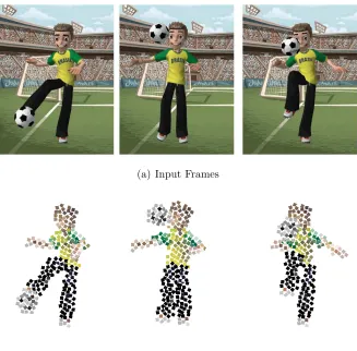
1.4 One example with animated mosaics: the input video shows a boy playing
soccer, shown in Figure (a). The resulting frames of the mosaic animation
are in Figure (b). The square tiles are moved from one frame to the next
according to the motion information detected at their center pixels, which
generates a temporally coherent motion effect. . . 9
Figure (b) are not aligned with the edge of the circle and the neighbouring
tiles have tile orientations not emphasizing the circular shape of the central
object. This results in a visually unappealing mosaic with large gap space
and blurred colours. Figure (c) shows a good tiling example, where tiles are
aligned with the shape of the circle and packed tightly. . . 10
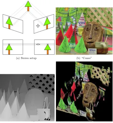
1.6 Examples of stereo: Figure (a) Stereo setup. The images are taken by two
synchronized cameras, and are rectified so that the cameras share the same
baseline parallel to their image planes. The two pixels marked by the black
squares are corresponding pixels, since they are both the projections of the
tree tip. By finding the correspondence between the pixels in the left and
right images, we can then compute the displacement of the pixels from right
to left image, which is also referred as “disparity”. In stereo, the disparities
are only in horizontal direction. Once the disparity is known, the depth of
the corresponding scene point can be found by triangulation. Figure (b)
shows the right image of a stereo image pair. Figure (c) shows the ground
truth for the disparities of the image given in Figure (b). And Figure (d)
shows the depth of the pixels in Figure (b). For each pixel in Figure (c),
the brighter is the intensity, the larger is the disparity, hence the closer is
to the camera, as shown in Figure (d). . . 14
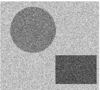
1.8 A synthetic example of our blob-like visual cues: Figure (a) illustrates the
right image of an artificial stereo pair. Notice there is little texture on both
the parallelogram and the background. Figure (b) shows the ground truth
for the disparity of the input image. The brighter is the pixel in Figure (b),
the larger is the disparity at that pixel. Figure (c) shows the blob-like visual
cues that our approach aims at. The pixels in the parallelogram belong to
the same blob-like visual feature, where the disparities are in a smoothly
varying range. The edges of this blob-like visual feature provide cues about
the disparities of the region they surround. However, for the background,
since we can not detect any visual cues on its boundary, there are no visual
cues detected in the background. This is indicated by the black pixels. . . 18
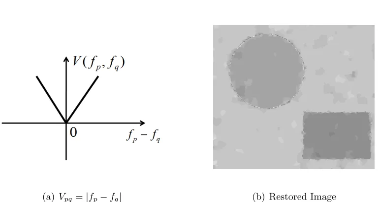
2.1 An Example of Image restoration: Figure (a) is the original image, where
both the objects and the background are of constant intensity. Figure (b)
shows the image corrupted with Gaussian noise (µ = 0 and δ = 0.05). L = {0,1,2, . . . ,255} is the label set. The restoration task is to assign a labell∈ Lto pixels in the image so that the noise is removed. . . 23
image for Figure 2.1(b). It is generated with Vpq = |fp − fq|. Notice the image is over-smoothed at the boundaries of the circle and the rectangle. We
histogram corrected the image in Figure (b) to illustrate the over-smoothing
effect. . . 25
2.3 Piecewise Constant Prior: Figure (a) is the Potts smoothness term, Vpq =
wpq ×T(fp 6= fq). Figure (b) shows the image restoration result for Fig-ure 2.1(b) produced with Potts smoothness term. It is the best solution for
this particular example, comparing with Figure 2.2(b) and Figure 2.4(b). 26
2.4 Piecewise Smooth Prior: Figure (a) shows the truncated linear smoothness
term,Vpq(fp, fq) = min(K,|fp− fq|). Figure (b) shows the image restoration result for Figure 2.1(b) produced with truncated linear smoothness term.
The result in Figure (b) is better than that of Figure 2.2(b), however, for this
example, the image restoration result generated with Potts smooth term,
see Figure 2.3(b) is the best among them. . . 27
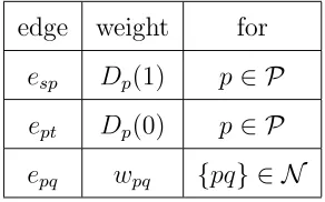
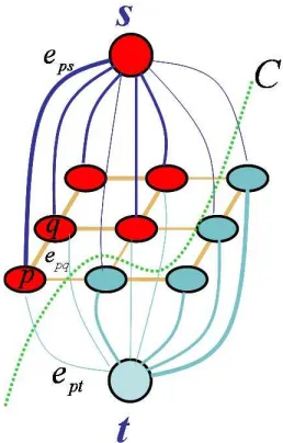
2.5 Graph cut demonstration on a 3×3 graph. The label set is{0,1}. Source
terminal s stands for label 0 and sink t stands for label 1. Each pixel in this graph is connected to terminals by t-links. The thickness of the t-links
represents how pixels like the corresponding label. For example, pixel p is linked tosby a thick edgeesp and a thin edgeept connectpto t. Therefore p is more likely to be assigned label 0. Vertices pq form an interacting pair. The weight of the n-link between p and q is large when pq are likely to have the same label. A cut C segments the vertices into two disjoint subsets, represented by different colors of the vertices. The label of each
pixel can be obtained by finding the subset which contains the pixel. This
constructions was first given by Greig et al. [32] . . . 33
connected to the two terminal nodes associated with label α and β. Let Pαβ =PαSPβ. For any pixel p ∈ Pαβ, the weights of the t-links between
p and the terminals α and β are: tαp = Dp(α) +Pq∈Np,q /∈PαβV(α, fq) and tβp =Dp(β) +Pq∈Np,q /∈PαβV(β, fq). The neighbouring pixels are connected with n-links. The weight of the n-link epq between any pair of pixels p and q isVpq(α, β). . . 38
2.9 An example of motion magnification. Figure (a) is from the input video
sequence where the bookshelf is pressed. The deformation of the bookshelf
is inevitable to human vision. Figure (b) is produce by the motion
magni-fication approach proposed by Liu et al. [61]. Compared with Figure (a), it
clearly reveals the deformation of the bookshelf. . . 41
2.10 The process of Liu et al. [61]. These images are from Liu et al. [61].. . . . 42
3.1 Hausner’s method. Figure (a) shows the input image. Figure (b) illustrates
the tile orientation field. Figure (c) shows the Centroidal Voronoi Diagram
computed with Manhattan distance and aligned with the tile orientation
field in Figure (b). Notice the CVD cells are pushed away from the curves
marked by the user, which are shown in white lines. Figure (d) is the final
result after putting the tiles centered at each cell of CVD. . . 50
necessary discontinuities or strange halo effect that ignores the background
details. . . 52
3.3 Shows R and B regions used in of Dalign p (ϕp). . . 58
3.4 Starry Night Results. . . 69
3.5 Portray Results . . . 71
3.6 Tiger Results. . . 72
3.7 Progression of mosaic stitching described in Section 3.5.2.2 . . . 73
3.8 Mosaics with different wv . . . 74
4.1 Two consecutive frames from the animation generated by Smith et al. [85]. 80 4.2 Summary of the approach. . . 82
4.3 Illustrates global label construction. Three frames that result from pairwise motion segmentation are shown. Three models are extracted between each pair of frames, i.e. k = 3. Different labels are illustrated by different colours. Notice that after pairwise motion segmentation, we do not know that the “red” model in frame 1 should correspond to the “green” model to in frame 2 and to the “yellow” model in frame 3. This should be discovered automatically. In practice, motion correspondences are not as easy to resolve as in this picture. Three global motion models extracted: purple (combines M11 and M22) brown (combines M12 and M23), and blue (combines M13 and M21 ). . . 88
4.4 User interaction and motion segmentation correction. . . 90
4.5 Several frames from aWalkingsequence and the corresponding classic mosaic. 93 4.6 Results on “Waving arms” sequence. . . 94
the matching cost is the sum of absolute differences. . . 105
5.2 Stereo with dynamic programming. In (a), the axes are left and right
s-canlines. The brightness of the squares shows the matching cost of
corre-sponding pixel pairs. The darker the square is, the greater the matching
error is. A path with the minimum matching cost is found from lower left
corner, shown by white squares. In (b), the axes are the left scanline and
disparities. A path from the fist column to the last column with minimum
cost is shown by white squares. . . 107
5.3 The results of Veksler [91]: Figure (a) is the left input image. Figure
(b) shows the dense feature detected at disparity 10. Figure (c) is the
dense feature for disparity 14. Figure (d) is the disparity assignment
after resolving the ambiguity. . . 112
its disparities vary smoothly. Figure (b) is the ground truth. Figure (c) is
the result generated by the approach of [91]. Pixels with black colour mean
there is no disparity assigned to them. This is because these pixels do not
belong to any dense feature. We can see that no visual correspondence is
found inside the big bowling ball in the middle because [91] only finds dense
features that belong to a single disparity. . . 113
5.5 The main steps of our semi-dense visual correspondence method. Figure (a)
is the input image. Figure (b) shows the sparse visual cues detected by our
classifier at disparity 35 and 49. The red pixels are the positive cues which
support disparity 35 and 49, and the green pixels are the negative cues which
do not support disparity 35 or 49. The black pixels neither like nor dislike
disparities 35 or 49. Figure (c) and (d) are two of our visual cue groups.
Here the blue pixels in Figure (c) show the cluster of positive visual cues
which support the range of disparities from 34 to 38. The yellow pixels in
Figure (d) are the visual cues which support disparity range from 48 to 52.
The green pixels are the negative cues which do not support these disparity
ranges. Figure(e) shows the binary labeling results for the visual cue groups
in Figure (c) and (d). Figure (f) is the final result after ambiguity resolving. 114
5.6 The training set for the sparse visual cues classifier: the ratiortextureof the textured pixels in Figure (a), (b), and (c) are 1.33%, 7.16%and 17.28%
re-spectively. Our training set covers examples from modestly textured images
to highly textured images. . . 121
5.7 The linkage clustering process: Figure (a) shows a synthetic example of six
positive visual cues. Figure (b) shows the linkage clustering process based
on the samples given in Figure (a).. . . 125
pixelbis included in both the blue and the green dense features. Therefore, we need to assign a label in {1,2} to pixel b. Pixel g is not covered by any dense visual feature, therefore, it is not assigned any label. The answer
to the multi-labeling problem is a semi-dense visual correspondence, where
each pixel either supports a disparity range or is not covered, as shown in
Figure (b). . . 131
5.9 Semi-dense correspondence with different group number K: Figure (a) is the result for K = 30. Notice the background is broken into several pieces. Figure (b) is the result for K = 10. In Figure (b), some small cones are over-grouped with the larger cones. . . 134
supports disparity 1 to 3. Blob S2 supports disparity 3 to 5, and blob S3 supports disparity 2 and 3. In Figure (b), blob S2 and S3 are grouped
to-gether. The new blobS2′ support disparity 2 to 5. The right part of Figure (c) shows the new dense features H1′ and H2′ generated based on the new grouping S′. The middle part of (c) shows the labeling process of the re-finement. The left part of (c) is the result after rere-finement. The new result
has two pixel blobs. The blue pixels support disparity 1 to 3, and the green
pixels supports disparity 2 to 5. . . 135
5.11 The testing set: Figure (a), (c), (e), and (g) are the right images of the
testing stereo pair. We want our testing set to cover images from highly
textured images to modestly textured images. Figure (b), (d), (f), and (h)
are the disparity maps of Figure (a), (c), (e), and (g). . . 139
5.12 The sparse visual cues for Tsukuba pair at disparity 10, 12, 16 and 21.
The green pixels do not support the associated disparity d, and the true disparities for these pixels are notdeither. They are classified correctly. The red pixels support the associated disparityd, and their true disparities are alsod. They are also classified correctly. The purple pixels are classified as the positive visual cues which support disparityd, but their true disparities are not d. The blue pixels should be classified as the positive visual cue since their true disparities ared. But our binary classifier misclassifies them as the negative visual cues. . . 140
5.13 The sparse visual cues for the Cones pair at disparity 21, 26, and 33. . . . 141
5.14 The sparse visual cues for the Bowling pair at disparity 26 and 62. Our
classifier is set to be biased towards the negative cues. Therefore, in Figure
(b), we have large false negative rates, shown with blue pixels. . . 142
Figure (a) is the visual cue group for the Bowling pair at disparity range
49 to 59. This is the disparity range of the big bowling ball in the middle.
Figure (b) is the dense visual feature generated based on the visual cue
group in Figure (a). . . 145
5.18 The initial semi-dense visual correspondence for the images in Figure 5.11.
Pixels with the same colour support the same range of disparities. Black
pixels are not assigned any disparity range, since there is no sparse visual
cue detected in these regions or on the boundaries of these regions. . . 146
5.19 The error rate and energy of the initial semi-dense visual correspondence.
The horizontal axe is the group numberK. The vertical axe in Figure (a) is the energy. The vertical axe in Figure (b) is the error rate Error(s). Generally, for the Bowling pair, Pots pair and Cones pair, the smaller isK, the lower is the error rate and the energy. However, for the Tsukuba pair,
it is reversed: the greater isK, the lower is the error rate, but the higher is the energy. . . 147
5.20 The refined semi-dense visual correspondence for the images in Figure 5.11.
Pixels with the same colour support the same range of disparities. Black
pixels are not assigned any disparity range. . . 148
number K. The vertical axe in (a) is the energy for the multi-labeling framework developed in Section 5.4.4. The vertical axe in (b) is the error
rate Error(S). When refining the results, as K decreases, the energy and the error rates do not always decrease. However, from these examples, we
can see that when the energy is small, it is highly possible the error rate is
small. . . 150
5.22 The results of Veksler [91]: Figure (a) to (d) show the results for Tsukuba,
Cones, Bowling, and Pots. Their coverage are 79%, 69%,26%, and 10%
respectively. The method in [91] works well in textured images, such as the
Tsukuba pair and the Cones pair. However, for images with large textured
regions, such as the Pots and the Bowling pair, the coverage of this method
is low, compared with our results in Figure 5.20.. . . 151
5.23 Comparison between our results and the results of Veksler [91]: Figure (a)
shows the input image which is highly textureless. Figure (b) shows our
result. The background is assigned the disparity range from 4 to 5. The big
bleach bottle on the right (the green blob) is assigned disparity range from 7
to 8. The wine bottle (pink blob) on the left is assigned disparity range from
6 to 7. The bleach bottle in the middle (the blue blob) is assigned disparity
range from 5 to 6. Our algorithm made gross error in the blue blobs, where
pixels that should be assigned the disparity range of the background are
assigned the disparities of the bleach bottle. Figure (c) shows the result
generated by the method in Veksler [91]. The disparities of the two bleach
bottles and the wine bottle are recovered. However, the disparities of the
table and the background are missing in Figure (c), as shown in black colour.152
1 Ada-boost for sparse visual cues . . . 123
2 Semi-dense visual correspondence . . . 138
Introduction
1.1
Energy Optimization in Computer Vision and
Graphics
Computer vision is the science and technology that enables the machines to see. Its
goal is to extract information from an image to “understand” a scene. Its applications
range from simple tasks such as counting the number of bottles on a production line
to the research in artificial intelligence and robotics with the goal to comprehend
the world around them. On the contrary, computer graphics manipulates the visual
content of the images to create digital synthesis of the real world. The main tasks
of computer graphics include representation of three-dimensional objects (geometry),
simulation of object deformation through time (animation), and generating realistic
or stylized images from models (rendering).
Traditionally, computer vision and graphics were two distinct fields since they focus
on different topics of interest. However, recently, with the emerging of new techniques
such as 3D television, telecommunication and virtual reality, vision and graphics are
address the issues such as visually displaying the results in high quality, modeling user
interaction with the environment naturally and intuitively. Since computer graphics
devotes a lot on real-world synthesis, such as photo-realistic rendering [20, 72, 2] and
object modeling [45, 88, 102], one successful approach is to use real images and 3D
scans, which are usually viewed as computer vision methods. Computer vision also
uses many techniques from computer graphics. For example, 3D modeling is widely
used in recognition systems for analysis and synthesis [9, 70]. In order to deal with
all these new challenges, we need to investigate the vision and graphics problems in
a new way which integrates these two fields.
Most problems in computer vision and graphics are very challenging. Due to the
ambiguities in visual interpretation, uncertainty and large dimensionality of the
da-ta, there are usually many possible solutions unless additional constraints from prior
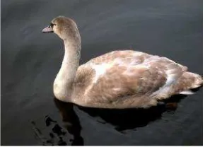
knowledge are imposed. Consider the image segmentation problem proposed in
Fig-ure 1.1. The task is to segment the light object (swan), from the darker background
(water). Thus we want to segment the lighter pixels as the swan and the darker
pixels as the background. Figure 1.1(b) to Figure 1.1(d) illustrate three different
possible solutions to this segmentation problem. It is easy for a human to conclude
that Figure 1.1(b) is the best solution among these three choices. However, an
au-tomatic computer vision system would need precise instructions on how to measure
the “goodness” of a solution. Thus some mechanism is required to evaluate all the
options and select the best one. The optimization approaches provide an expressive
way to solve this problem.
There are usually two major steps in the optimization framework. The first step is to
formulate an objective function. The objective function maps any solution to a real
number, this number being a measure of how good the solution is. A good objective
function should incorporate the constraints that an acceptable solution must satisfy.
The objective function should assign high goodness score to solutions that match the
(a) The task is to segment the swan from the water
(b) Good Segmentation: the object is shown in red and the background with green.
(c) Deviation from observed images: ob-serve the region inside the black circle. A great number of pixels are segmented as the swan. Comparing with (a), these pixels in fact have more similar colour to the water than to the swan. Segmenting these pixels as the object violates the data constraint.
(d) Deviation from prior knowledge: the swan and background shapes are not coher-ent, with many tiny “holes”. This violates our prior knowledge that these object and background shapes tend to be contiguous in space.
(a) Objective Function (b) Energy Function
Figure 1.2: An example of objective function and energy function for the image segmenta-tion problem in Figure 1.1: Figure (a) is a possible objective funcsegmenta-tion. Notice the solusegmenta-tion in Figure 1.1(b), namely b, is assigned higher goodness score than c and d in Figure 1.1(c) and Figure 1.1(d). In this work, we usually refer the objective function as an energy function. Energy functions assign low energy to good solutions, as shown in Figure (b).
constraint and prior constraint. The data constraint comes from the observed data. It
requires a desired solution to be close to the observed data. For example, in Figure 1.1,
it is easy to come up with the constraint that the pixels that belong to the object
should have lighter colours and the background pixels should have darker colours.
Otherwise they are violating the data constraint provided by the colour information
of the image. The prior constraint is from our prior knowledge about a physically
plausible solution to the problem. Most physical world objects are coherent in space,
that is for most pixels in the object, all nearby pixels also belong to that object. In
this case, our prior knowledge tells us that both the background and the object should
be spatially coherent. We can encode more prior constraints in the energy functions,
such as a preference to a particular shape, say a round shape prior, which encourages
the object to have a round shape.
The second step of the optimization approach is to minimize the energy function.
This is also a very challenging problem. Since computer vision and graphics usually
deals with images and videos, the problem size is huge. It is impossible to find the
optimal solution by simple enumeration. Moreover, the energy functions are usually
not convex, which makes it hard to find their minima by using standard minimization
knowledge to solve the problem by encoding it in the energy function. Thus we can
expect the desired solution to have some nice global properties, such as the overall
smoothness in the image segmentation example in Figure 1.1. Finally, the value of
the energy function provides an effective way to evaluate the solution and can be used
as a guide in the optimization algorithm.
Great effort has been made towards developing effective energy optimization
algo-rithms. Among all these approaches, graph cut algorithm [12, 13, 53] has been proven
to be an effective tool for computer vision and graphics applications. As a global
op-timization method, the graph cut algorithm can find the exact minimum of certain
energy functions (the everywhere smooth prior [44], defined in Section 2.1). For a
wider range of energy functions (e.g. piecewise smooth prior, defined in Section 2.1)
which are NP-hard to optimize, it can find a local minimum within known factor from
the optimal [12]. Although the class of energy functions that can be optimized by the
graph cut approach is restricted, it is useful enough to be applied to a wide range of
vision and graphics problems.
In this thesis, we address two graphics and vision applications: rendering artificial
classic mosaics and finding semi-dense cues for visual correspondence. We formulate
both the animated mosaic problem and visual correspondence problem in the energy
optimization framework. Graph cut algorithm is used as the energy optimization tool
functions in these two applications, together with how we adapt our energy functions
so that they can be optimized by graph cuts.
1.2
Artificial Classic Mosaics
1.2.1
Still and Animated Mosaics
Computer graphics is not only about simulating realistic images, a large area of
graphics is devoted to creating artful effects to enhance the images taken from the
real world. For example, people often use tools such as Photoshop to create different
effects on the real world pictures so that the result images may be more appealing to
the user. There are also tools helping the users to create art works, such as artificial
oil paints, line drawings and mosaics etc. With all these tools based on computer
vision and graphics techniques, more ordinary people will be given the freedom of
creating their own art work. The users would be even more interested if one can
create animations of their own, with computer aided tools.
Non-photorealistic rendering (NPR) is an area of comptuer graphics which deals with
rendering real world photographs in an artistic style. NPR rendering creates stylized
images by arranging drawing primitives, for instance painting strokes, line segments or
tiny dots, in an artful way. The purpose of NPR is to assist humans in creating digital
art and to render images in such a way that the important information that they
contain in emphasized. Recently, there has been a great interest in non-photorealistic
rendering, such as artificial line drawing [24, 25], digital painting [68, 54, 39], stippled
drawing [82, 21, 71], and classic mosaics [36, 23, 63, 64].
Mosaic is one of the most durable and ancient art forms. As early as ancient Roman
times, people use this durable art forms to decorate walls, ceilings and furniture etc.
It is usually composed of thousands of primitives, such as colourful stones, ceramic
Figure 1.3: Classic mosaic example: Christ surrounded by angels and saints, from basilica of Sant’Apollinare Nuovo in Ravenna, Italy. Notice inside the red rectangle, the artist broke the square tiles into irregular shapes to adapt to the image.
the drawing primitives of a mosaic image, namely the “tiles”, have square or rectangle
shape, then this mosaic belongs to the category of classic mosaic. Figure 1.3 shows an
example of classic mosaics. Simulating static mosaics from digital images is one area
of non-photo-realistic rendering and it has been widely investigated, see [36, 23, 5, 64].
As already mentioned above, one goal of NPR rendering is to create images with a
more profound impact on the viewer. It is even more true for an NPR animation, since
it has one more dimension(time) of expressiveness. Although there are great number
of works on static NPR rendering, such as [24, 25, 39, 36, 64], relatively little work
has been done towards generating NPR animations automatically or iteratively [85,
mosaic effects from real video.
Little work has been reported on generating mosaic animations automatically,
es-pecially for animated mosaics from real video. The animations generated by our
approach are composed of hundreds of colourful square tiles, which are arranged to
present the shape and colour of the objects inside the given video, moving in a timely
coherent manner. Each frame of the resulting animation is a classic mosaic image
composed of a great number of square tiles, which are located along the important
edges inside the given scene. Between the consecutive frames, the tiles are moved
according to the motion of their center pixels. Therefore, the whole animation will
have a consistent motion effect.
Figure 1.4 shows a synthetic example of our desired mosaic animation. The input
video shows a boy playing soccer. The resulting frames of the mosaic animation
are shown in Figure 1.4(b). The square tiles are moved from one frame to the next
according to the motion information detected at their center pixels, which generates
a temporally coherent motion effect.
Our method estimates the motion of the pixels inside the video, renders the frames
with mosaic effect based on both the colour and motion information from the input
video. We aim at a tool that requires minimal help from the user to finish the task
of generating animated mosaics. We hope with the help of our animation tool, more
people will be able to create their own mosaic animation without professional training.
1.2.2
Constraints on Static and Animated Mosaics
Most of the work on rendering static mosaics is inspired by observing the artists. To
obtain a visually appealing mosaic, there are some basic rules that almost all methods
follow. First, the edges of the mosaic tiles should be parallel to the important edges
of the underlying image, as shown in Figure 1.5(c). Which edges are essential can be
(b) Mosaic Frames
Figure 1.4: One example with animated mosaics: the input video shows a boy playing soccer, shown in Figure (a). The resulting frames of the mosaic animation are in Figure (b). The square tiles are moved from one frame to the next according to the motion information detected at their center pixels, which generates a temporally coherent motion effect.
of curves to indicate the objects they want to emphasize in the images, such as the
work of Hausner [36] and of Elber and Wolberg [23]. The others, for instance, the
work of Di Blasi et al. [10] and Battiato et al.[6], adopt edge detection algorithms to
generate a set of principal curves and use them as the guide lines for tile orientation.
Besides these two approaches, some of the static mosaic approaches encode the edge
information as a soft cue when computing the tile orientations, such as Liu et al. [64]
and Battiato et al. [5].
(a) input image (b) bad mosaic (c) good mosaic
Figure 1.5: A synthetic example of a good and a bad mosaic: Figure (a) shows the synthetic input image. Figure (b) shows a bad tiling example. The tiles inside Figure (b) are not aligned with the edge of the circle and the neighbouring tiles have tile orientations not emphasizing the circular shape of the central object. This results in a visually unappealing mosaic with large gap space and blurred colours. Figure (c) shows a good tiling example, where tiles are aligned with the shape of the circle and packed tightly.
as tightly as possible, see Figure 1.5(c). It is NP-hard to find the optimal solution
to the tile packing problem, since it can be considered as a bin packing problem.
Many previous works on rendering classic mosaics are based on heuristics, such as
Hausner [36], Elber and Wolberg [23], and Battiato et al. [5]. However, it is still
possible to find an approximate good solution, after transforming the tile packing
problem into a labeling problem.
While it is possible to create simple animations with mosaic effects manually, it is very
challenging to create animated classic mosaics automatically from real video. There
are two main difficulties in rendering animated mosaics from video. First, each frame
of the animated mosaics should itself be an appealing static mosaic. Thus animated
mosaics have to obey all the constraints for a static mosaic: the tile orientation
should be parallel to the principal edges in the input image, and the tiles should
be packed tightly to minimize the gap space inside the mosaic. Second and more
important, to create the animation effect, the motion of the tiles must be spatially
and temporally consistent. For example, two neighbouring tiles on the right arm of
the boy in Figure 1.4(b) should move with similar velocity through all the frames.
We improve our previous work on classic static mosaics [63] by addressing this problem
in a more principled global energy minimization framework. Our main contribution
to the area of non-photorealistic rendering is our animated mosaic method. Most
previous works on generating non-photorealistic animations, such as the work of Klein
et al. [50], require the users to provide the motion information for the rendering
primitives. This is a very tedious work even for very short video clips. Moreover,
rendering primitives are usually deformed during the animation process, for instance,
in the work of Litwinowicz [60]. Our goal is to generate animated classic mosaics
without the user providing full motion information. The constraints on classic mosaic
also require that the mosaic tiles are not deformed in any case. Therefore, the previous
methods on rendering NPR animations can not be applied to our animation problem.
Unlike the work of Smith et al. [85], we render animated mosaics from real video
sequences. As already mentioned, one of the main challenges is to make sure there
is a temporal coherence in the animation. One way to achieve temporal coherency
is to displace groups of tiles in a consistent manner. For this purpose we develop
a new motion segmentation algorithm with occlusion reasoning. Our algorithm
re-quires minimal help from the user. We pack the tiles into the discovered coherent
motion layers, using colour information in all the frames in a global manner. Our
tile packing algorithm is based on the one for still mosaic proposed by Liu et al. [64],
rendering static mosaics as a global energy optimization frame work in Chapter 3.
Occlusions are handled gracefully. We produce colourful, temporally coherent and
uniquely appealing mosaic animations. We believe that our method is the first one
to animate classic mosaics directly from video.
1.3
Semi-dense Visual Correspondence
1.3.1
Visual Correspondence
In order to create a faithful mosaic animation, the motion of the pixels inside the given
video must be estimated accurately. Rendering each frame individually without the
motion information leads to unpleasant “flickering” effects which are disturbing to the
viewer. Motion estimation is usually performed by finding the visual correspondence
between consecutive frames. In the visual correspondence problem, we are given two
images of the same real world scene. A pixel in one image is said to correspond to a
pixel in the other image, if these two pixels are projections along the lines of sight of
the same physical scene element, see Figure 1.6. The problem is to find pairs of such
corresponding pixels.
In stereo, the real world is captured by synchronized cameras from distinct view
points. The straight line connects the optical centers of these two cameras is called
the baseline. Usually it is assumed that this baseline is parallel to the image planes for
both cameras after rectification. Corresponding points are found between these two
images, see Figure 1.6(a). The difference in the locations of corresponding pixels seen
in the left and right images, often referred as “disparity”, is used to determine the
depth1 of these pixels. The disparities for stereo problem are only in the horizontal
dimension, which means the corresponding pixels are in the same scanline. This
1Here “depth” means the distance between the world point corresponding to the pixel and the
Figure 1.6(b). And Figure 1.6(d), taken from [103], shows the depth of the pixels in
Figure 1.6(b). For each pixel in Figure 1.6(c), the brighter is the intensity, the larger
is the disparity, hence the closer is to the camera, as shown in Figure 1.6(d). The
problem of finding visual correspondence is still not a well solved problem after many
years of investigation. This, together with our need to find more accurate motion
for the tiles for mosaic animation, inspires us to extend our research into the field
of finding visual correspondence. Most methods intended for stereo correspondence
are easily extended to motion correspondence, however stereo correspondence has
a simpler setup. Thus although our intent is to develop visual correspondence for
motion sequences, we begin by investigating correspondence for stereo.
1.3.2
Visual Correspondence: Main Challenges
Finding the visual correspondence is a very challenging problem. To get the correct
visual correspondence, a lot of problems have to be overcome. For instance, image
noise will bring errors in when measuring the difference between corresponding pixel
pair. Other problems can be caused by sampling artifacts, exposure change, motion
blur, etc. Among all these problems, lack of texture and occlusions are two of the
hardest problems to solve when computing the visual correspondence. First, in
(a) Stereo setup (b) “Cones”
(c) Disparity map for “Cones” (d) Depth for “Cones”
right image since the wall part where it is located on is occluded by the ball in the
right image. The blue dots are the neighbouring pixels of pixel p′. In Figure 1.7(b),
we enlarge pixels p, p′ and the neighbours of p′ to show their intensity. As shown in
the Figure 1.7(a), pixel pandp′ locate in a region with little texture. The neighbours
of p′ also have very similar intensity with pixel p, which makes it hard to decide the
true disparity ofp. Pixelqis actually occluded by the bowling ball in the right image. Therefore its disparity can not be determined without further assumptions about the
scene.
A lot of research has been devoted to solve these problems. The existing approaches
can be mainly divided into two categories. On one hand, correspondence can be found
by using sparse feature points. These methods obtain promising results in regions
with texture cues, but their results can be too sparse to be used in some applications
such as image-based rendering. Dense correspondence approaches estimate disparity
at every pixel but can have gross errors in some parts of textureless areas. Worse still,
most dense approaches do not produce confidence maps for their estimates, that is
they do not say which parts of the disparity maps they are more confident in. That
is the motivation for the proposed method. Our main objective is to find semi-dense
visual correspondence in the areas of an image where disparities can be found more
(a)
(b)
Figure 1.7: An example for occlusion and textureless regions: Figure (a) shows the input stereo image pair. Pixel p and pixelq are two pixels in the left image, located on the same scanline. Here we use yellow and red dots to show their positions. Pixel p′ corresponds to p in the right image, but pixel q does not have correspondence in the right image, it is occluded by the ball. The blue dots are the neighbouring pixels of pixel p′. In Figure (b), we enlarge pixel p, p′ and the neighbours of p′ to show their intensity. As shown in the Figure (a), pixel p and p′ locate in a region with little texture. The neighbours of p′ also have very similar intensity with pixelp, which makes it hard to determine the true disparity of p.
1.3.3
Semi-dense Visual Correspondence
The difficulties in finding visual correspondence are caused by many reasons,
includ-ing image noise, image samplinclud-ing artifacts, textureless regions and occlusions. It is
well known that a reliable visual correspondence cue can be found more easily in
the textured regions. This is because the intensity changes provide more information
about the reliability on the matching quality of the corresponding pixel pairs. This
es-image pair. Notice there is barely any texture on the parallelogram or in the
back-ground. Figure 1.8(b) shows the ground truths for the disparity of the input image.
The brighter is the pixel in Figure 1.8(b), the larger is the disparity at that pixel.
Figure 1.8(c) shows the semi-dense visual correspondence detected by our approach.
The pixels in the parallelogram belong to the same semi-dense visual feature. Unlike
that of [90] and [91], whose blob-like visual cues only have one disparity for each, our
blob-like visual cues have a smoothly varying range of disparities. The edges of this
semi-dense visual feature provide more confident information about the disparities
of the region they surround. Since there is no visual cues detected on the boundary
of the background or in its interior, our approach can not detect any dense visual
features in the background.
1.3.4
Motivation and Contribution
Our work of finding semi-dense visual cue was inspired by the work of Veksler [91,
90]. For stereo and motion detection, the main difficulty is the ambiguity brought
by texturelessness or repeating texture. No matter using local methods or global
methods2, it is hard to decide the correct disparity for the pixels inside the textureless
2Informally, in local methods, one pixel may look at the nearby pixels in a small neighbourhood
(a) Right image of the input
stereo pair (b) Ground truth (c) Blob-like visual cues
Figure 1.8: A synthetic example of our blob-like visual cues: Figure (a) illustrates the right image of an artificial stereo pair. Notice there is little texture on both the parallelogram and the background. Figure (b) shows the ground truth for the disparity of the input image. The brighter is the pixel in Figure (b), the larger is the disparity at that pixel. Figure (c) shows the blob-like visual cues that our approach aims at. The pixels in the parallelogram belong to the same blob-like visual feature, where the disparities are in a smoothly varying range. The edges of this blob-like visual feature provide cues about the disparities of the region they surround. However, for the background, since we can not detect any visual cues on its boundary, there are no visual cues detected in the background. This is indicated by the black pixels.
region, since more then one possible disparities will give little or even zero matching
error, see Figure 1.7.
However, reliable cues can be found at the border of the textureless regions. This can
be done by comparing the matching error with the strength of the intensity edges.
If the matching error is less than the edge strength at a particular pixel by some
threshold, as mentioned in [91], then this feature can be used as a trustable cue for
the stereo and motion detection. The threshold of selecting the visual correspondence
cues is picked by hand in the work of [91] and [90]. In our work, we developed a
learning framework that select useful features to decide the locations of these visual
cues automatically, which avoids the problem of selecting fixed threshold. More useful
features other than the difference between matching error and edge strength can
be easily included in our learning frame work. We construct a feature pool of 148
step into several groups, based on their geometric location and associated disparities.
The resulting feature groups contain sparse cues for consecutive disparities. And the
sparse visual cues in the same group are also geometrically close to each other. We
also use graph cut algorithm to propagate the information brought by the visual cues
in the feature groups into textureless regions. This step is done for each feature group
individually. And the results are semi-dense feature blobs for groups of consecutive
disparities.
The final step is ambiguity resolving. One pixel inside the input image pair can
belong to more than one semi-dense feature blobs generated in the previous step. To
find the exact boundaries of these semi-dense cues, we apply α-expansion algorithm to resolve the ambiguities between the semi-dense feature blobs. This step produces
nice boundaries between regions of the images with different groups of disparities.
Textureless regions are also covered by our approach, which produces more evidence
to the disparities of these regions.
1.4
Thesis Organization
In Chapter 2 we describe the energy optimization framework, followed by the
in-troduction to the graph cuts algorithm, from the aspects of different constraints of
global energy optimization framework. We first formulate the energy formulation on
the static mosaic problem. Then we provide the approach of optimizing the energy
function. In Chapter 4, we will go through the details about rendering animated
mo-saics from real video. We show how we perform motion segmentation with occlusion
handling, together with how we modify our static mosaic rendering methods for the
animation problem. In Chapter 5, we will describe how we extract semi-dense visual
cues from stereo image pair. We propose a method which extracts useful features in
the textured regions of the input image for finding visual correspondence, followed by
our clustering approach to grouping all the sparse features detected in the previous
step. We apply graph cut algorithm to propagate our features into textureless regions
Energy Optimization with Graph
Cuts
In this chapter, we will describe the framework of energy optimization method based
on graph cuts, which in the last several yeas has become a widely utilized optimization
approach in computer vision and graphics. In Section 2.1 we will first present some
labeling problems in Computer Vision and Graphics, and the energy formulation for
solving them, followed by the common constrains for these problems. Next, we will go
through some energy optimization approaches which are widely used, such as dynamic
programming, simulated annealing and gradient descent.
In Section 2.2, we will give the overview of Graph Cut algorithm at first. Then,
from the aspect of different constraints on the labeling problems to solve, we will
go through variations of energy optimization methods based on graph cuts. In the
last section, Section 2.3, we briefly describe some applications in vision and graphics
2.1
Energy Optimization in Vision and Graphics
In this section, we will show how certain vision and graphics problems can be stated as
labeling problems, and how energy functions can be formulated to evaluate the quality
of the labeling. We will also describe the common constraints for these labeling
problems, such as everywhere smooth constraint, piecewise smooth constraint and
piecewise constant constraint. We will illustrate how these constraints can be encoded
in the energy functions associated with the labeling problems. Moreover, we will
introduce some commonly used algorithms in optimizing these energy functions.
2.1.1
Labeling Problem and a Common Form of Energy
Func-tions
Many problems in vision and graphics can be naturally represented as labeling
prob-lems. For example, if one wishes to segment an object of interest from its
back-ground, then each pixel can be labeled as either background or foreback-ground, denoted
correspondingly by labels 0 and 1. This type of a problem with two labels is called a
binary labeling problem.
Many other problems can be viewed as multi-labeling problems, for instance, the
image restoration problem shown in Figure 2.1. Figure 2.1(a) illustrates the original
image with a light background and two objects with constant intensity. Figure 2.1(b)
is the corrupted image with Gaussian Noise (µ = 0 and δ = 0.05). A label set L = {0,1,2, . . . ,255} represents all possible gray scale intensity levels. To restore the original image, a label fp ∈ L will be assigned to each pixel pin the image. Let
f = {fp|p ∈ P} denote the collection of all pixel label assignments. If f is close enough to the original image, then the noise is reduced and original image is restored.
(a) Original Image (b) Noisy Image
Figure 2.1: An Example of Image restoration: Figure (a) is the original image, where both the objects and the background are of constant intensity. Figure (b) shows the image corrupted with Gaussian noise (µ= 0 and δ= 0.05). L={0,1,2, . . . ,255} is the label set. The restoration task is to assign a label l ∈ L to pixels in the image so that the noise is removed.
where L is a finite label set. A commonly used constraint is that the labels should vary smoothly almost everywhere. Labels are allowed to change drastically in a few
places, and this is very important in order to preserve sharp discontinuities that may
present.
Energy functions are formulated to evaluate the solutions to these labeling
problem-s, under the constraint of smoothness over the image which comes from our prior
knowledge as well as other constraints. We will discuss some common types of the
smoothness constraints later. An additional constraint comes from the observed data.
Letf be a labeling that assigns each pixelp∈ P a labelfp ∈ L. Usually the following energy function is formulated to evaluate the quality of f:
E(f) =Esmooth(f) +Edata(f) (2.1)
which f is not smooth. Edata, usually called the data term, measures how pixels in P like the labels that f assigns them.
Edata is often formulated as
Edata(f) =
X
p∈P
Dp(fp)
whereDp is the penalty for assigning pixelpthe labelfp. For example, for binary seg-mentation, suppose we expect the object to have intensity of 40 and the background
to have intensity of 200. Then we can setDp(1) = (Ip− 40)2 andDp(0) = (Ip− 200)2, where Ip is the intensity of pixel p, 1 is the object label, and 0 is the background label.
A typical choice of Esmooth is
Esmooth =
X
{pq}∈N
Vpq(fp, fq) (2.2)
Usually, N consists of pairs of immediately adjacent pixels, that is the interactions are given by the standard 4-connected grid. Longer-range interactions can be also
included in N. The choice of Vpq is critical. In most cases, it should make f vary smoothly in most places while preserving the discontinuities at object boundaries.
How to set up Vpq depends on our prior knowledge about the smoothness of the desired labeling. There are several widely applied constraints on Vpq. Here we list three major types.
The everywhere smooth prior has a small penalty for labeling that is smooth
(a) Vpq=|fp− fq| (b) Restored Image
Figure 2.2: Everywhere Smooth Prior: Figure (a) shows an example of the everywhere smooth prior, the absolute distance Vpq = |fp − fq|. Figure (b) is the restored image for Figure 2.1(b). It is generated with Vpq =|fp− fq|. Notice the image is over-smoothed at the boundaries of the circle and the rectangle. We histogram corrected the image in Figure (b) to illustrate the over-smoothing effect.
this labeling will not be penalized too much. Therefore, the optimal labeling is not
likely to have drastic changes between any pair of neighbouring pixels. The problem
with the everywhere smooth prior is that for most labeling problems in vision and
graphics, there should be some tolerance for sharp label changes on the boundaries
of the objects, so that they can restore the data around the discontinuities correctly.
Otherwise, these discontinuities are over-smoothed, see Figure 2.2.
Piecewise Constant Prior: Some computer vision and graphics problems require
different labels for neighouring pixels at object boundaries, but within the object,
the pixels should have same labels. Consider the example of the image restoration
problem illustrated in Figure 2.1. Both the objects and the background have constant
intensities. We need to preserve the discontinuities at the boundaries of these objects,
that means we should allow sharp changes at the edges of the regions of background
and the objects. However, within each object and the background, the labels should
(a) Vpq=wpq×T(fp6=fq) (b) Restored Image
Figure 2.3: Piecewise Constant Prior: Figure (a) is the Potts smoothness term, Vpq = wpq×T(fp6=fq). Figure (b) shows the image restoration result for Figure 2.1(b) produced with Potts smoothness term. It is the best solution for this particular example, comparing with Figure 2.2(b) and Figure 2.4(b).
assign label 127 to every pixel, which is the true intensity of the circle. The piecewise
constant prior assigns a low cost to such labeling.
A good choice for piecewise constant prior is the so called Potts Model, which is
Vpq(fp, fq) = wpq ·T(fp 6= fq), see Figure 2.3(a). Here T(fp 6= fq) is 1 if fp 6= fq and 0 otherwise. Potts smoothness term is most appropriate for non-ordered labels
or when the number of labels is small. Figure 2.3 shows the image restoration result
generated with piecewise constant prior. For this particular example, since both
the background and the objects are of constant intensity, piecewise constant prior
is a more appropriate choice compared to the everywhere smooth prior.. Therefore,
comparing with the results generated with everywhere smooth prior, see Figure 2.2(b)
and piecewise smooth prior, see Figure 2.4(b), piecewise constant prior produces much
better solution to the image restoration problem.
Piecewise Smooth Prior: There are also computer vision and graphics problems
(a)Vpq(fp, fq) = min(K,|fp− fq|) (b) Restored Image
Figure 2.4: Piecewise Smooth Prior: Figure (a) shows the truncated linear smoothness term, Vpq(fp, fq) = min(K,|fp − fq|). Figure (b) shows the image restoration result for Figure 2.1(b) produced with truncated linear smoothness term. The result in Figure (b) is better than that of Figure 2.2(b), however, for this example, the image restoration result generated with Potts smooth term, see Figure 2.3(b) is the best among them.
each object or region, the labels should vary smoothly. For instance, for stereo, at the
boundaries of the objects, one should alow the disparity labels to change drastically.
But within each object, the disparity of the pixels should be able to vary smoothly to
form a smooth surface, and also restore the data. To make a discontinuity preserving
Vpq, one typically “truncates” the function by setting Vpq(fp, fq) = min(K,|fp− fq|), where K is the truncation constant, see Figure 2.4(a). In this way, the penalty for a discontinuity is never larger than K, and sharp discontinuities can be created, see Figure 2.4.
Many discontinuity preserving energy functions have been proposed in [33, 57, 89]. In
addition to specifying smoothness assumptions, the choice forEsmoothalso dictates the choice of optimization algorithm and as the result the quality of optimization that can
linear and the Potts Vpq lead to an energy which is NP-hard to optimize [53], but there are approximation algorithms with different quality guarantees, see [12]. We
will describe some of these algorithms in Section 2.2.
To solve these labeling problems related to the vision and graphics applications,
en-ergy functions presented in Equation 2.1 must be optimized. Unfortunately, many of
these energy functions are not convex and they have many local minima. Worse still,
the labeling f usually has dimension |P|to the power of|L|, which is thousands asP is the set of pixels in an image. The computational cost of getting global minima of
these energies represented in Equation 2.1 is enormous. It forces researchers to find
efficient but approximate optimization algorithms.
2.1.2
Optimization algorithms
Over the years, researchers have been working on finding good energy optimization
algorithms. In this section, we will briefly describe some commonly used optimization
methods.
Gradient descent is an algorithm which can find a local a minimum of a function.
The idea behind gradient descent is taking steps in the direction of negative gradient
of the function. This makes the function decrease fastest and then reach a local
minimum. There are two problems with gradient descent. Firstly, the convergence
of this approach is not guaranteed. The choice of step width is the critical issue
of gradient descent algorithm. When the steps are too large, the function may not
converge. If the step width is too small, it will take too many steps to reach a
local minima, which results in an enormous computational cost. Worse still, there is
no general guidance to find a good step width and make sure the gradient descent
algorithm converges in an acceptable time. The biggest drawback of gradient descent
is that it can only reach a local minimum of the energy function. The global minimum,
find a better solution.
The simulated annealing algorithm is an analogue to the physical annealing process.
It is the only general-purpose method to find, or in most cases, to approximate the
best solution to the energy optimization problems. It starts from a random initial
labeling. At each iteration of simulated annealing, the labeling at one particular
pixel is changed locally and randomly. The annealing schedule is controlled by the
temperature parameter, T, which is set to be a high value and gradually decreased during the annealing process. If the energy is decreased with the local change, then the
new labeling is accepted. In case of energy increasing, the probability of accepting
the new labeling is then determined partially by the temperature parameter. The
higher the temperature, the larger is the probability of accepting the change. The
probability of accepting a new labeling with higher energy than the current labeling
prevents the algorithm from being stuck at a local minimum. When the temperature
is high, the simulate annealing algorithm performs more like a random walk. As the
temperature decreases during the annealing process, the algorithm tends to look for
a local minimum. There is a certain order to visit the pixels.
The temperature parameter is decreased according to a cooling schedule. If the
cool-ing schedule is optimal, simulated annealcool-ing will obtain a global minimum. However,
it is prohibitively expensive to perform simulated annealing under the optimal
running time. In this case, only a local minimum of the energy function can be found
with simulated annealing.
Dynamic programming can be applied to energy optimization when the energy
function has a very restricted form. It solves a complex problem by breaking it down
into simpler subproblems. The solution of a given optimization problem must be able
to be obtained by the combination of optimal solutions of the subproblems. And
any recursive algorithm solving the original problem should solve the subproblems by
breaking them down into simpler problems, rather than generating new subproblems
of same complexity. Therefore, dynamic programming requires that the problem to
be solved must have one-dimensional structure rather then loopy structures. This
includes some important cases, such as snakes [48]. The two dimensional energy
functions that arise in low level vision can not, in general, be solved efficiently via
dynamic programming except some special cases [28].
Graph cuts can be applied to find the global minimum for certain two-dimensional
energy functions and find good approximate solutions of certain other energy
func-tions. In the following section, we will describe how graph cut algorithm is used to
optimize different energies.
2.2
Graph Cuts
The graph cut algorithm has been widely used in Computer Vision and Graphics
for the purpose of energy optimization. It has been proved to be successful in many
situations. In this section, we will describe the graph cuts algorithm and how it
is used to optimize different energies, together with some examples in vision and
The cost of a cut C is defined as:
|C|=X e∈C
we
The cut with minimum cost is called the minimum cost cut. There are two main
approaches to solving Min-Cut/Max-flow problem for the two-terminal graphs. In
Cormen et al. [15], an “augmenting path” strategy is described to compute the
min-imum cut of a graph. An alternative approach named “push-relabel” is presented
in Goldberg and Tarjan [31] to solve the minimum cut problem. Theoretically, the
computational cost of minimum cut algorithms is a low order polynomial. Boykov
and Kolmogorov present a comparative study of standard minimum cut algorithms
in [13]. They also provide a new minimum cut algorithm in [13] and in practice their
algorithm is significantly faster than other standard algorithms for graphs arising from
computer vision problems. For our implementation, we use the algorithm in [13], and
its implementation is provided by the authors.
2.2.2
Energy optimization with graph cuts
Energies which can be optimized through graph cuts usually have the following form:
E(f) = X p∈P
Dp(fp) +
X
{pq}∈N