Article
Multivariable Static Output Feedback Control of a
Binary Distillation Column using Linear Matrix
Inequalities and Genetic Algorithm
Kalpana R. 1, Harikumar K. 2*, Senthilkumar J. 1, Balasubramanian G. 1, and Abhay S. Gour 3
1 School of Electrical and Electronics Engineering, SASTRA University, Thanjavur, Tamilnadu, India; e-mail:
[email protected]; [email protected]; [email protected].
2 School of Electrical and Electronic Engineering, Nanyang Technological University, Singapore; e-mail:
[email protected]; [email protected].
3 Centre for Cryogenic Engineering, Indian Institute of Technology, Kharagpur, India; e-mail:
* Correspondence: [email protected]; [email protected]; Tel.: +6590547402
Abstract:The current work addresses the control of two-input two-output (TITO) Wood and Berry 1
model of a binary distillation column. The controller design problem is formulated in terms of 2
multivariableH∞control synthesis. The controller structure takes the form of simplest static output 3
feedback (SOF) control. The controller synthesis is performed using a hybrid approach of blending 4
linear matrix inequalities (LMI) and genetic algorithm (GA). The performance of the static output 5
feedback controller is compared with three other controllers designed for Wood and Berry model 6
available in the literature. The first simulation study is performed for the case of tracking a unit 7
step command in the presence of a step change in output disturbance. A second simulation study is 8
performed for rejecting a change in sinusoidal output disturbance. 9
Keywords:Distillation column, Disturbance rejection, Genetic algorithm,H∞control, Linear matrix 10
inequalities, Static output feedback. 11
1. Introduction 12
Multivariable chemical processes are arduous to control due to the coupling between multiple 13
input channels and multiple output channels. Distillation control is a challenging problem due 14
to inherent non-linear nature of the process, severe coupling between various inputs and outputs, 15
nonstationary behavior of the process and effect of unmeasured disturbances. In this paper, we 16
address the issue of multivariable nature of the distillation control having interaction among different 17
control loops and the effect of unmeasured output disturbances. Wood and Berry proposed a popular 18
two-input two-output (TITO) transfer function model of a pilot scale binary distillation column 19
[1]. A plethora of multivariable control techniques are available in the literature, applied to TITO 20
model of binary distillation column proposed by Wood and Berry, [2]-[9]. A method based on the 21
static decoupler design using the steady state gain matrix is proposed in [2]. The decentralized 22
proportional-integral-derivative (PID) controller designed for the decoupled process is then combined 23
with the static decoupler to yield a multivariable controller. A similar methodology of decoupling 24
followed by design of decentralized controllers are discussed in [3] - [9]. The performance of the 25
decentralized controllers depends upon the degree of decoupling achieved. Under the ubiety of strong 26
coupling between the different control loops, the performance of decentralized controller degrades. 27
Multivariable control design techniques inherently handle the coupling related issues found common 28
in distillation control. 29
In this paper, a multivariable static output feedback (SOF) controller is designed using a hybrid 30
approach of blending linear matrix inequalities (LMI) and genetic algorithm (GA). Static output 31
feedback control has found a lot of applications due to the ease in practical implementation [10] - [14]. 32
LMI is a powerful tool for synthesizing output feedback controllers satisfying multiple requirements. 33
Multiple objectives like robust pole placement,H2/H∞performance measures and frequency domain 34
specifications can be easily realized through a system of LMI’s [15] - [20]. The conventional solution of 35
LMI’s utilizes convex programming methods [21]. Multi-objective design requirements often leads to a 36
system of bilinear matrix inequalities (BMI). In this paper, BMI is transformed to LMI by restructuring 37
the additional slack variable of BMI as an input variable to GA. The solution provided by GA evolves 38
over several iterations based on probabilistic rules and leads to an optimal/suboptimal solution [22]. 39
The paper is organized as follows. Section 2, discuss about the transfer function and state space model 40
of Wood and Berry distillation column. A multivariableH∞control formulation is given in section 3. 41
An algorithm for the synthesis of SOF controller is given in section 4. Section 5 discusses the simulation 42
results, comparing the performance of SOF controller with other three controllers available in the 43
literature for Wood and Berry distillation column. Section 6 concludes the paper. 44
2. Model of Binary Distillation Process 45
The TITO transfer function model for methanol-water separation in a distillation column is given in equation1, [1]. The controlled variables (outputs) are the composition of top product (Y1) and bottom product (Y2), expressed in percentage of methanol in weight. The manipulated variables (control inputs) are the reflux steam flow rate (U1) and the reboiler steam flow rate (U2) in the units of lb/min. All the time constants are expressed in the unit of minutes (min).
Y1(s) Y2(s)
!
=
12.8e−s
16.7s+1
−18.9e−3s
21s+1 6.6e−7s
10.9s+1
−19.4e−3s
14.4s+1
!
U1(s) U2(s)
!
(1)
Using a first order Pade-approximation for time delay in equation1yields a rational transfer function for the distillation column model as given in equation2.
Y1(s) Y2(s)
!
= g11(s) g12(s)
g21(s) g22(s)
!
U1(s) U2(s)
!
(2)
The expression for the termsg11(s)tog22(s)are given in equations from3to6.
g11(s) = 12.8
(−0.5s+1)
(16.7s+1)(0.5s+1) (3)
g12(s) =
−18.9(−1.5s+1)
(21s+1)(1.5s+1) (4)
g21(s) = 6.6
(−3.5s+1)
(10.9s+1)(3.5s+1) (5)
g22(s) =
−19.4(−1.5s+1)
(14.4s+1)(1.5s+1) (6)
The state space model of the system given in equation2is given in equations7and8. TheAmatrix for the state space model is given in equation9. TheBmatrix for the state space model is given in equation10andCmatrix is given in equations11.
˙
Y=CX (8) A=
−2.06 −0.479 0 0 0 0 0 0
0 0 0 0 0 0 0 0
0.25 0 0 0 0 0 0 0
0 0 −0.378 −0.210 0 0 0 0
0 0 0.125 0 −0.714 −0.127 0 0
0 0 0 0 0.25 0 0 0
0 0 0 0
0 0 0 0 0 0 −0.736 −0.185
0 0 0 0 0 0 0.25 0
(9) B= 2 0 0 0 1 0 0 0 0 2 0 0 0 2 0 0 (10)
C= −0.383 3.066 0 0 0.45 −1.2 0 0
0 0 −0.606 1.384 0 0 0.674 −1.796
!
(11)
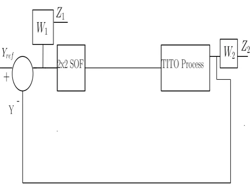
3. MultivariableH∞control formulation 46
Optimization inH∞space is suitable for systems having uncertainty in dynamics and disturbances. A 47
diagram representing theH∞control formulation for the binary distillation column is given in figure1. 48
Along with the weighted sensitivity function (S), weighted complementary sensitivity function (T) is 49
also minimized leading to multi-objective design problem [24]. Generic form of the weightsW1(s)and 50
W2(s)are given in the equations12and13respectively. The weighting functionW2(s)is taken as high 51
pass filter to attenuate the detrimental effects of unmodeled dynamics at higher frequencies. To retain 52
good tracking and disturbance rejection properties at low frequencies, an ideal choice for the weighting 53
functionW1(s)is a low pass filter. The performance outputs to be minimized areZ= [Z1,Z2]and are 54
W
1W
2Z
1Z
2+
-2x2 SOF
Y
refY
TITO Process
Figure 1.Diagram representingH∞control formulation.
W1(s) = We1
(s) 0
0 We2(s)
!
(12)
W2(s) =
Wy1(s) 0
0 Wy2(s)
!
(13)
Z1= [Ze1,Ze2]
T (14)
Z2= [Zy1,Zy2]
T (15)
The linear state space equation for the generalized plant are given in equations16to19. Generalized 56
plant is obtained by augmenting the state space model of binary distillation column given in equations 57
7to11with the weighting transfer functionsW1(s)andW2(s). In equations16to19,Xtgis the state
58
vector of the generalized plant, Y is the vector of measurements (Y1andY2),Utcis the vector of control
59
inputs (U1andU2) andWtdis the vector of disturbance inputs. The disturbance inputsWtdcorresponds
60
to the reference inputsY1re f andY2re f.
61
˙
Xtg= AtgXtg+BtuUtc+BtwWtd (16)
62
Z1=Ct1Xtg+Dt11Utc+Dt12Wtd (17)
63
Z2=Ct2Xtg+Dt21Utc+Dt22Wtd (18)
64
Selection of weighting transfer functionsW1(s)andW2(s)follow the guidelines presented in [23]. The 65
low pass filter weightsWe1(s)andWe2(s)are given in equations20and21respectively. The high pass 66
filter weightsWy1(s)andWy2(s)are given in equations22and23respectively. 67
We1(s) =
0.1
(s+0.2) (20)
We2(s) =
0.1
(s+0.3) (21)
Wy1(s) =
0.01(s+0.1)
(s+2) (22)
Wy2(s) =
0.01(s+0.1)
(s+3) (23)
The objective of the control design problem is to synthesis a SOF controller with the structure,Utc=KY
that minimizes the norm given in equation24.
kTzwtd k∞=k
W1S W2T
!
k
∞
(24)
4. Static output feedback controller synthesis using LMI 68
Applying SOF controlUtc=KYfor the system given in equations16to19, the resulting state space
69
model for the closed loop generalized plant are given in equations25to27. 70
˙
Xtg= (Atg+BtuKCt)Xtg+BtwWtd (25)
71
Z1= (Ct1+Dt11KCt)Xtg+Dt12Wtd (26)
72
Z2= (Ct2+Dt21KCt)Xtg+Dt22Wtd (27)
LetAclt = Atg+BtuKCtbe the closed loop system matrix. The Lyapunov condition for stability of
73
the closed loop system can be written as the following matrix inequality given in equation28, [17]. 74
In equation28,Q = AcltTP+PAclt, M = NBtuBtuTPandR = BTtuP+KCt,Pis a positive definite
75
matrix andNis any square matrix. The matrix inequality given in equation28is bilinear. The bilinear 76
matrix inequality (BMI) in equation28can be converted into LMI by fixing one of the unknownsPor 77
N. Since there is a constraint onP(P>0),Nis taken as a decision variable for genetic algorithm (GA). 78
ChoosingNas the decision variable for GA instead ofPis less conservative and results in a enlarged 79
search space. Multiple choices forNis selected by GA and the resultant LMI is solved by minimizing 80
a performance index. The performance index is given in equation29. 81
Q−M−MT+NBtuBtuTN RT
R −I
!
<0 (28)
The variablesqt1andqt2in equation29, takes the binary value 0 or 1 based on closed loop stability 82
requirements. The binary value of variablesqt1andqt2are obtained as follows. Letγclidenote theith
83
eigenvalue of the closed loop system matrixAclt, letngcltbe the dimension ofAcltandRe(γ)denotes 84
the real part of the complex variableγ. 85
CASE I IFRe(γcli)>=0, for any i= 1, 2, 3, ...,ngclt, THENqt1=1 andqt2=0. 86
CASE II IFRe(γcli)<0,∀i= 1, 2, 3, ...,ngclt, THENqt1=0 andqt2=1. 87
Therefore, either JPI=100 or 0<JPI<1 (sincekTzwtd k∞ ∈ (0, 1)). The SOF control gains are found
88
iteratively using the algorithm given below. 89
90
1. Choose N as decision variable and JPIas the performance index for GA.
91
2. Solve the LMI given in equation28to obtain P and K for the value of N given by GA. 92
3. Evaluate the performance index JPI, given in equation29.
93
4. Iterate the steps 1,2 and 3 until JPIis minimized.
94
5. Numerical simulation results and discussion 95
For solving the LMI given by the equation28, the matrixNis set to a diagonal matrix. Table1gives 96
the initialization details of the genetic algorithm toolbox in MATLAB 7.5. The SOF gain obtained is 97
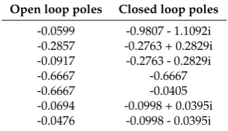
given in equation30withkTzwtdk∞=0.498. A comparison of open loop poles and closed loop poles
98
of the system given in equations7to11is given in Table2. Please note that there is no one to one 99
correspondence between the open loop and closed loop poles given in Table2. The SOF gain stabilizes 100
the closed loop system and also minimizeskTzwtdk∞.
101
Table 1.Initialization of GA toolbox in MATLAB 7.5.
Attibute Value
Population size 500 Population range [-20,20] Number of generations 100
Selection function Stochastic uniform Crossover function Scattered
Mutation function Gaussian
K= −0.8145 0.6059
−0.2200 0.3025
!
(30)
Table 2.Open loop and closed loop poles
Open loop poles Closed loop poles
-0.0599 -0.9807 - 1.1092i -0.2857 -0.2763 + 0.2829i -0.0917 -0.2763 - 0.2829i
-0.6667 -0.6667
-0.6667 -0.0405
-0.0694 -0.0998 + 0.0395i -0.0476 -0.0998 - 0.0395i
A comparative study is conducted to evaluate the performance of the SOF controller with the other 102
given in equation1is simulated in SIMULINK for a time duration of 100 minutes. As a first case, a 104
step change in output disturbance is given in bothY1andY2from a time instant of 50 minutes. The 105
objective is to track a unit step command in bothY1andY2channels simultaneously in the presence of 106
a step output disturbance acting in both of the output channels. The performance is quantified in terms 107
of integral square error (ISE) in trackingY1andY2and also the integral square value (ISV)of control 108
inputsU1andU2. An expression for ISE and ISV are given in the equations31and32respectively 109
(similar equations are used forY2andU2). Please note that the integration is performed numerically 110
using SIMULINK with a fixed time step used for simulation. 111
ISE=
Z 100
0 (Y1−Y1re f)
2dt (31)
ISV=
Z 100
0 U1
2dt (32)
Figure2gives the outputY1and figure3gives the outputY2respectively of various controllers in 112
tracking a unit step command in both of the output channels (Y1andY2), in the presence of a unit step 113
change in output disturbance in both of the output channels. The solid blue curve shows the response 114
of the SOF controller given in equation30. The response of the controllers presented in [2], [3] and [4] 115
is given by black curve (dashed), brown curve (dotted) and green curve (dash-dot) respectively. After 116
the introduction of output disturbance at a time instant of 50 minutes, the response of SOF controller is 117
superior in terms of lowest undershoot and smallest settling time when compared to other controllers. 118
The steady state error for tracking is poor for SOF controller for initial 50 minutes due to the lack of 119
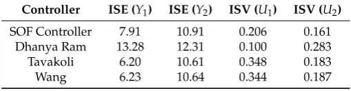
integrator. The performance metric ISE and ISV is given in Table3for the case of tracking a unit step 120
command in both of the output channels (Y1andY2), in the presence of a unit step change in output 121
disturbance in both of the output channels. The performance of the controllers designed in [3] and [4] 122
are similar, but consumes very large control input when compared to SOF controller. Clearly, the SOF 123
controller outperforms the one designed in [2]. Unmeasured output sinusoidal disturbances of very 124
small frequencies are also prominent in process control applications. Figure4gives the outputY1and 125
figure5gives the outputY2respectively of various controllers, in the presence of a sinusoidal change in 126
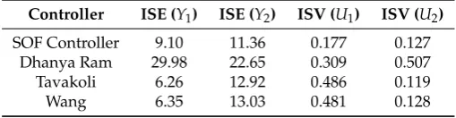
output disturbance of frequency 0.1 rad/min in both of the output channels. The performance metric 127
ISE and ISV is given in Table4for the case of rejecting a sinusoidal change in output disturbance of 128
frequency 0.1 rad/min in both of the output channels. The sinusoidal disturbance rejection property 129
of SOF controller is comparable to that of the controller designed in [3] and [4] and superior to the 130
one designed in [2]. From Table4, clearly the control effort (ISV ofU1) is on the lower side for SOF 131
Figure 2. Comparison of the performance of various controllers under step change in output disturbance (Y1).
Figure 3. Comparison of the performance of various controllers under step change in output disturbance (Y2).
Table 3.Results for a step change in output disturbance.
Controller ISE (Y1) ISE (Y2) ISV (U1) ISV (U2)
SOF Controller 7.91 10.91 0.206 0.161 Dhanya Ram 13.28 12.31 0.100 0.283
Tavakoli 6.20 10.61 0.348 0.183
Figure 4.Comparison of the performance of various controllers under sinusoidal change in output disturbance (Y1).
Figure 5.Comparison of the performance of various controllers under sinusoidal change in output disturbance (Y2).
Table 4.Results for sinusoidal change in output disturbance of frequency 0.10 rad/min.
Controller ISE (Y1) ISE (Y2) ISV (U1) ISV (U2)
SOF Controller 9.10 11.36 0.177 0.127 Dhanya Ram 29.98 22.65 0.309 0.507
Tavakoli 6.26 12.92 0.486 0.119
Wang 6.35 13.03 0.481 0.128
6. Conclusions 133
Design of multivarable static output feedback controller for a binary distillation column is presented 134
in this paper. The method adopted for controller synthesis is generic and can be applied to any 135
has excellent disturbance rejection properties with low control effort. The comparative study with 137
other controllers shows the performance and effectiveness of the controller. The simple structure 138
of the controller yields accurate practical implementation when compared to other higher order 139
controllers. Linear matrix inequalities are powerful tool for designing multivariable static output 140
feedback controllers and further design constraints can be easily incorporated to yield better control 141
solutions. 142
Author Contributions: Kalpana and Harikumar formulated the problem and written the manuscript. 143
Senthilkumar, Balasubramanian and Abhay. S. Gour did the simulations and also edited the manuscript. All the 144
authors have read and approved the manuscript. 145
Conflicts of Interest:The authors declare no conflict of interest. 146
Abbreviations 147
The following abbreviations are used in this manuscript: 148
149
BMI Bilinear matrix inequality GA Genetic algorithm ISE Integral square error ISV Integral square value LMI Linear matrix inequality SOF Static output feedback TITO Two input two output 150
References 151
1. Wood, R. K.; Berry, M. W. Terminal composition control of a binary distillation column.Chemical Engineering 152
Science. 1973, vol. 28, issue 9, pp. 1707-1717. 153
2. Dhanya Ram, V.; Chidambaram, M. Simple method of designing centralized PI controllers for multivariable 154
systems based on SSGM.ISA Transactions. 2015, vol. 56, pp. 252-260. 155
3. Tavakoli, S.; Griffin, I.; Fleming, P.J.; Tuning of decentralised PI (PID) controllers for TITO processes.Control 156
Engineering Practice. 2006, vol. 14, issue 9, pp. 1069-1080. 157
4. Wang, Q. G.; Huang, B.; Guo, X. Auto-tuning of TITO decoupling controllers from step tests.ISA Transactions. 158
2000, vol. 39, issue 4, pp. 407-418. 159
5. Iruthayarajan, M. W.; Baskar, S. Evolutionary algorithms based design of multivariable PID controller.Expert 160
Systems with Applications. 2009, vol. 36, issue 5, pp. 9159-9167. 161
6. Hajare, V. D.; Patre, B. M. Decentralized PID controller for TITO systems using characteristic ratio assignment 162
with an experimental application.ISA Transactions. 2015, vol. 59, pp. 385-397. 163
7. Nandong, J.; Zang, Z. Multi-loop design of multi-scale controllers for multivariable processes.Journal of 164
Process Control, 2014, vol. 24, issue 5, pp. 600–612. 165
8. Chang, W. D. A multi-crossover genetic approach to multivariable PID controllers tuning.Expert Systems 166
with Applications, 2007, vol. 33, issue 3, pp. 620-626. 167
9. Avila, S.T.; Gutiérrez, A.J.; Hahn, J. Analysis of Multi-Loop Control Structures of Dividing-Wall Distillation 168
Columns Using a Fundamental Model.Processes, 2014, vol. 2, pp. 180-199. 169
10. Wang, N.; Pei, H.; He, Y.; Zhang, Q. Robust H2 static output feedback tracking controller design of
170
longitudinal dynamics of a miniature helicopter via LMI technique. 24th Chinese Control and Decision 171
Conference. 2012, Taiyuyan, China, pp. 346-350.DOI: 10.1109/CCDC2012.6244051.
172
11. Harikumar, K.; Arun Joseph, Seetharama Bhat, M; Omkar, S.N. Static output feedback control for an 173
integrated guidance and control of a micro air vehicle.Journal of Unmanned System Technology. 2014, vol.2, 174
No. 1, pp. 17-29. 175
12. Kong, Y.; Zhau, D.; Yang, B.; Shen, T.; Li, H.; Han, K. Static output feedback control for active suspension 176
using PSO-DE/LMI approach.IEEE international Conference on Mechatronics and Automation. 2012, Chengdu, 177
13. Komnatska, M.M. Flight control system design via. static output feedback: LMI approach. 2nd IEEE 179
International Conference on Actual Problems of Unmanned Air Vehicles Developments. 2013, Keiv, Ukraine, pp. 180
184-186,DOI: 10.1109/APU AVD.2013.6705320. 181
14. Doye, I.N.; Voos, H.; Darouach, M.; Schneider, J.G.; Knauf, N. Static output feedback stabilization of nonlinear 182
fractional order glucose insulin system.IEEE EMBS International Conference on Biomedical Engineering and 183
Sciences, 2012, Langkawi, Malaysia, pp. 589-594.DOI: 10.1109/IECBES.2012.6498043.
184
15. Scherer, C.; Gahinet, P.; Chilali, M. Multiobjective output feedback control via. LMI optimization. IEEE 185
Transactions on Automatic Control, 1997, vol. 42, no. 7, pp. 896-911. 186
16. Chilali, M.; Gahinet, P.; Apkarian, P. Robust pole placement in LMI regions.IEEE Transactions on Automatic 187
Control. 1999, vol. 44, no. 12, pp. 2257-2269. 188
17. Cao, Y.Y.; Lam, J.; Sun, Y.X. Static output feedback stabilization: an ILMI approach.Automatica. 1998, vol. 34, 189
no. 12, pp. 1641-1645. 190
18. Fujimori, A. Optimization of static output feedback using substitutive LMI formulation.IEEE Transactions on 191
Automatic Control, 2004, vol. 49, no. 6, pp. 995-999. 192
19. He, Y.; Wang, Q.G. An improved ILMI method for static output feedback control with application to 193
multivariable PID control. 2006,IEEE Transactions on Automatic Control, vol.51, no. 10, pp. 1678-1683. 194
20. Lee, D. H.; Joo, Y. H.; Kim, S. K. A Proposition of Iterative LMI Method for Static Output Feedback Control 195
of Continuous-Time LTI Systems.International Journal of Control, Automation and Systems. 2016, vol. 14, no. 4, 196
pp. 1-7. 197
21. Boyd, S.; Ghaoui, L.E.; Feron, E.; Balakrishnan, V. Linear matrix inequalities in system and control theory. 198
SIAM, Studies in Applied Mathematics. 1994, vol. 15, pp. 12-18. 199
22. Haupt, R.L.; Haupt, S.E. Practical genetic algorithms.Wiley Interscience. 2004, pp. 27-47, 2004. 200
23. Jiankun, H.; Bohn, C.; Lu, H.R. SystematicH∞weighting function selection and its application to the 201
real-time control of a vertical take-off aircraft.Control Engineering Practice. 2000, vol. 8, issue 3, pp. 241-252. 202
24. Skogestad, S.; Postlethwaite, I. Multivariable feedback control, Analysis and design.John Wiley and Sons. 203
2001, pp. 309-394. 204