MULTIPLE INPUT MULTIPLE OUTPUT CHANNEL
MEASUREMENTS AND SYSTEM PERFORMANCE
Michael Mewburn
A THESIS SUBMITTED IN FULFILMENT OF THE REQUIREMENT FOR THE DEGREE OF MASTER OF ENGINEERING
AT
CENTRE FOR TELECOMMUNICATIONS AND MICRO-ELECTRONICS, VICTORIA UNIVERSITY
DECLARATION
“I, Michael Mewburn, declare that the Master by Research thesis entitled “Multiple Input Multiple Output channel measurements and system performance” is no more than 60,000 words in length, exclusive of tables, figures, appendices, references and footnotes. This thesis contains no material that has been submitted previously, in whole or in part, for the award of any other academic degree or diploma. Except where otherwise indicated, this thesis is my own work”.
Michael Mewburn ______________________________________
C
ONTENTS
Contents ... ii
Abstract ... v
Acknowledgements ... vii
Mathematical Notation ... viii
Chapter 1 ... 1
Introduction ... 1
1.1 Background ... 1
1.2 Literature review ... 3
1.3 Contribution of the thesis ... 5
1.4 Thesis overview ... 6
Chapter 2 ... 7
Multiple Input Multiple Output Communication ... 7
2.1.1 Limitation of SISO capacity ... 8
2.1.2 Multipath propagation conditions ... 9
2.1.3 Coherence bandwidth and time dispersion characteristics of multipath channels. ... 9
2.2 Operating principles of MIMO Communication systems ... 12
2.3 Cost / benefit considerations ... 13
2.4 Propagation model ... 14
2.5 Singular Value Decomposition ... 14
2.5.1 Sub channel redundancy ... 16
2.6 MIMO capacity ... 16
2.7 Normalisation ... 18
Chapter 3 ... 20
Hardware Development and Operation ... 20
3.1 Development goals ... 21
3.2 Hardware description ... 22
3.2.1 Receiver... 24
Omnidirectional receive array ... 24
Directional receive array ... 25
3.2.2 Ancillary Receive array hardware ... 25
Power supply ... 26
RF switch ... 26
RF switch controller ... 27
Low noise amplifiers ... 28
3.2.3 Transmitter ... 29
Displacement accuracy ... 31
3.2.4 Network Analyser ... 31
3.2.5 Master PC ... 32
3.2.6 Measurement Software ... 32
Data storage ... 34
3.2.7 Antenna development ... 35
Discone ... 35
Circular dipole (directional) array ... 37
Dual polarised patch... 38
3.3 Measurement programs ... 41
3.5 Data quality ... 43
3.5.1 Hardware Calibration ... 44
Calibration procedure ... 45
Chapter 4 ... 48
Results and Analysis ... 48
4.1 Analysis software ... 48
4.2 Channel stability ... 52
4.3 Indoor channel frequency response ... 53
4.3.1 Variation in measured channel gain... 55
4.4 Indoor MIMO channel capacity ... 55
4.4.1 Path Loss and array element directivity ... 56
Capacity calculated with fixed SNR ... 57
Capacity calculated with measured SNR ... 61
4.4.2 Array element polarisation ... 63
Transmit array ... 64
Receive array ... 65
Results ... 65
Examination of MIMO gain in isolation... 65
Examination of MIMO gain and channel gain combined ... 66
4.4.3 Channel correlation ... 66
4.5 Singular value comparison of a range of indoor MIMO channels ... 68
4.6 Keyhole effect ... 70
Chapter 5 ... 71
Conclusion ... 71
Further work ... 73
Publications ... 74
References ... 75
Appendix A ... 79
Appendix B ... 84
Appendix C ... 89
Appendix D ... 90
A
BSTRACT
Existing wireless links using a single antenna element at the transmitter and receiver are heavily influenced by the multipath scattering arising from objects in the transmission environment. Unlike conventional systems, a concept referred to as Multiple-Input Multiple-Output or MIMO not only thrives under multipath conditions but also has the potential to allow for substantial increases in capacity. MIMO systems use a combination of multiple antenna arrays at the transmitter and receiver in conjunction with dedicated Digital Signal Processing (DSP). Before MIMO systems are designed and deployed, a database of typical propagation measurements is required to confirm theoretical predictions with reality.
The design, development and use of specialised measurement equipment to accurately establish an indoor MIMO measurement database is presented in this thesis. An extension of this work is the consideration of practical hardware choices (for example antenna type) in an end user implementation.
I
NFORMATION THEORETIC
CAPACITY
(
MAXIMUM
ERROR FREE CAPACITY
UTILISING IDEAL CODING
)
AND SINGULAR VALUE
ARE THE PRIMARY TOOLS
WITH WHICH
COMPARISONS BETWEEN
THE MEASURED CHANNELS
ARE MADE
.
T
HIS THESIS
DEMONSTRATES THAT FOR
THE GIVEN INDOOR
PROPAGATION
ENVIRONMENT
,
SIGNAL TO
NOISE RATIO IS A
SIGNIFICANT
DETERMINANT OF INDOOR
MIMO
CAPACITY AND
THAT OMNIDIRECTIONAL
ARRAY ELEMENTS AFFORD
CAPACITY THAN
DIRECTIONAL
ALTERNATIVES
.A
CKNOWL
EDGEMENTS
I am indebted to the Australian Telecommunications Cooperative Research Centre for funding assistance with this project and the following people for their generous assistance and support:
My supervisory team of Mike Faulkner, Phil Conder, Terence Betlehem and Ying Tan have gone above and beyond to help ensure the success of this research project and I thank them sincerely
Thanks are also due to the technical support team of Nghia Truong and Donald Ermel. Nghia was most helpful in producing printed circuit boards and running the measurement system, while Donald made his excellent machining skills available in the construction of the antenna positioning system and discone antennas.
Stewart Jenvey from the Centre for Telecommunications and Information Engineering at Monash University generously provided the directional receive array and the services of his anechoic chamber for antenna testing.
Inger Mewburn kindly proofread this work, offering valuable feedback.
M
ATHEMATICAL
N
OTATION
α nR
χ aggregate measurement hardware response matrix
x 1 frequency response vector of the low noise amplifiers
g is the transmit power amplifier response vector
hij
H
random fading between the ith receive element and the jth transmit element
◊ measured n
R x nT
H actual channel response matrix - In this work, H
complex channel matrix - includes hardware artefacts
◊
L n
after hardware correction
R x nR
i.i.d. independent and identically distributed
the Insertion loss and leakage matrix of RF switch
k number of singular values yielded by SVD(H) n length nR
n
AWGN vector
R
n
number of receive antenna elements
T
ρ SNR.
number of transmit antenna elements
s transmit element separation (number of multiples of λ/4 @ 2.45 GHz) σk kth
Σ diagonal singular value matrix
singular value
U unitary matrix V unitary matrix y length nR
x length n
receive vector
T transmit vector
Chapter 1
1 Chapter 1
I
NTRODUCTION
PREFACE
Chapter 1 discusses limitations of traditional wireless communication techniques and proposes an alternative method to improve reliability and data capacity, called multiple input, multiple output, or MIMO. The development and use of MIMO measurement hardware to characterise a typical indoor office propagation environment are presented as the contributions of this research project. The chapter concludes with a thesis overview to acquaint the reader with the document.
1.1
Background
(
SNR)
BW C= log21+
where the maximum channel capacity, C (bits/s) is proportional to the signal bandwidth, BW (Hz) and received signal to noise ratio, SNR. The wireless system discussed by Shannon consists of a single radiating element at either end of a communication link, now described as single input, single output or SISO.
The escalating consumer demand for reliable, high data rate wireless communication systems has for some time reached and indeed, pushed beyond the boundaries of the Shannon limit. Even with optimal coding and modulation schemes, these SISO communication systems must still comply with Shannon’s limit as an upper bound on capacity. The SISO topology has been the benchmark format for telecommunication of the twentieth century but is now being challenged by an alternative scheme, MIMO.
Multiple input, multiple output or MIMO communication systems utilise multiple element antenna arrays at the transmitter and receiver to offer significant capacity gains over SISO. Multiple element arrays have been successfully employed at the receiver for some time in the interests of diversity gain; where the best individual, or an optimal combination of several spatially separated receive elements is selected for maximal SNR. While improved SNR will increase capacity beyond that provided by a true SISO system, the Shannon limit still applies. By contrast, a multiple-input multiple-output (MIMO) system allows the simultaneous parallel transmission of multiple streams of data over the same bandwidth. MIMO has the potential to provide a linear increase in capacity proportional to the smaller number of transmit or receive array elements [2]. Systems employing simple antenna diversity furnish only a logarithmic capacity improvement.
Indoor- and heavily built up outdoor-environments are commonly considered to have rich or dense scattering properties due to the potentially large number of objects in and around the propagation path. Physical objects may cause reflection, refraction or attenuation (or any combination of the three) in the propagating wave. Attenuation lowers received SNR, in turn reducing capacity for both SISO and MIMO systems. Reflection and refraction can result in multiple time-delayed copies of the transmitted data arriving at the receiver; a phenomenon termed multipath. The
arbitrary phase addition at a receive antenna due to multipath results in random fading, or attenuation, of the received signal. Using any of a number of signal processing algorithms, MIMO systems utilise a rich scattering environment to de-correlate signal paths from spatially separated array elements. In addition to the potentially substantial increases in capacity, reliance upon multipath in MIMO inherently provides immunity to it.
A database of typical propagation measurements is required to validate theoretical predictions before the design and deployment of MIMO systems. Early research has depended upon propagation measurements and models based on SISO communication systems, but this lacks important information required for MIMO research. MIMO system designers require intimate knowledge of the propagation channel to evaluate the MIMO capacity improvement over SISO and to determine any hardware and environmental dependency. This project seeks to assess the effects of system characteristics such as antenna type, array configuration [3], access point location and building design and building materials [4] on MIMO systems.
1.2
Literature review
From infancy in the 1970s, the concept of increased capacity using multiple -antenna arrays gained significant momentum from the late 1980s and through the 1990s with seminal works by Winters [5], Foschini & Gans [2] and Telatar [6]. In these papers and numerous others since, channel capacity is examined with the aid of simulated channel responses in the absence of real measurement data.
This project was intended to amend the deficiency of actual measurement results (prior to commencement) available to researchers with an indoor propagation measurement campaign.
Literature pertinent to this research usually examines topics such as how synthetic models may be fitted to physical data and how physical parameters such as element spacing and location effect capacity. Much has also been said about the requirement for large amounts of scattering to sufficiently de-correlate the channel [9, 21]. The implication from this is that Non Line of Sight (NLOS) scenarios will be most conducive to MIMO channel capacity as the more highly correlated Line of Sight (LOS) components are not present. Some work has been carried out that suggests this is not always the case [22, 23], where it was found that good signal to noise ratio arising from an LOS scenario can play a significant role in determining capacity.
Some debate also appears evident over the optimum array element spacing [3, 9, 24, 25]. Correlation is shown to increase dramatically with increasing numbers of elements added to the same fixed aperture [24]. Contrary to this, it is claimed in [3] that a capacity increase may be observed between 0.5 and 0.2 wavelengths.
An obvious implication of the use of multiple element arrays in communication systems is the increase in physical array size and hardware complexity as the number of antennas and associated RF chains rises. Multimode MIMO systems have been proposed in [26] and others, where array size is significantly reduced or fully condensed to one element while still retaining the functionality of a full array. This is achieved by exciting two or more electromagnetic modes of the antenna(s); an approach suffering none of the cross coupling inherent between physically separate array elements. The significant benefits of this method are packaging and cost, as the number of transceivers and antenna elements are reduced. Another potential technique for reducing array dimensions is the switched parasitic antenna [27]. Parasitic elements, near the driven element are left open-circuit or shorted, with the number of combinations available corresponding to the number of virtual elements. The primary drawback of this system is the increase in SNR required to achieve the same capacity as a traditional array. Where the principal concern is the number of transceivers and not necessarily array elements, adaptive selection of sub arrays of the main array is made for each of the x < nR RF chains at
1.3
Contribution of the thesis
This project is concerned with the development of a MIMO measurement system (and use thereof) to extensively characterise an indoor propagation environment. The principle aims of this research project are:
• Develop a methodology for generating an indoor MIMO measurement database; involving the design, construction and testing of the appropriate radio channel measuring equipment. The accuracy of the measurements should be consistent with current and future requirements of indoor wireless communication systems.
• Undertake several measurement programs to comparatively study the effects of array configuration and array element types for typical indoor conditions.
• Develop Graphical User Interface based software to evaluate the performance of several MIMO systems using the gathered data.
The research project involves the development of a significant amount of hardware for the collection of channel measurements, comprising a mobile transmitter, stationary receiver and network analyser that together, measure the channel gain between each pair of transmit and receive antennas. The receiver is a fixed array where, depending on the array in question, one of four (or one of eight) antenna elements is multiplexed to the network analyser. The transmit array is synthesised with a single antenna mounted on a two-dimensional positioning system.
Purpose-specific software has been written in the MATLAB environment to analyse data measured by the network analyser, allowing comparison between measured channel performance and theoretical predictions of channel capacity. The software calculates and displays time and frequency domain representations, singular value behaviour and channel capacity for the user-defined MIMO channel.
The analysis software, antenna elements, omnidirectional receive array, transmit antenna positioning system and software to control them were developed specifically for this project.
high integrity, requiring careful design and implementation of the channel measurement program. The measurements must be essentially noise free and reproducible.
1.4
Thesis overview
The document is arranged as follows:
Chapter 2 - Multiple Input Multiple Output communication.
The theory and execution of MIMO wireless systems is described. Benefits and limitations of the concept are discussed and relevant literature is reviewed.
Chapter 3 - Hardware development and operation.
The development and implementation of the measurement apparatus is described. Operational requirements of the hardware necessary to achieve the goals of this work are covered. Detailed descriptions are given of individual hardware components and the software written to control them. All the mechanics, electronics, control software and calibration processes were developed by the author.
Chapter 4 - Results and analysis.
The MIMO measurement campaign data is presented and analysed using MATLAB software specially written by the author for the task. Theoretical aspects such as singular value decomposition and the calculation of capacity are discussed. The performance of many indoor MIMO wireless channels is evaluated, primarily in terms of singular value behaviour and MIMO capacity.
Chapter 5 - Conclusions.
Chapter 2
2 Chapter
M
ULTIPLE
I
NPUT
M
ULTIPLE
O
UTPUT
C
OMMUNICATION
PREFACE
2.1
The motivation for MIMO
Of particular interest for communication system design is the ability to reliably send and receive data with sufficient capacity (bits/s/Hz). Reliable reception with adequate capacity is of critical importance in typical propagation environments such as office spaces and heavily built up urban areas. The random fading inherent in these conditions reduces the capacity and reliability of reception for traditional SISO communications systems.
2.1.1 Limitation of SISO capacity
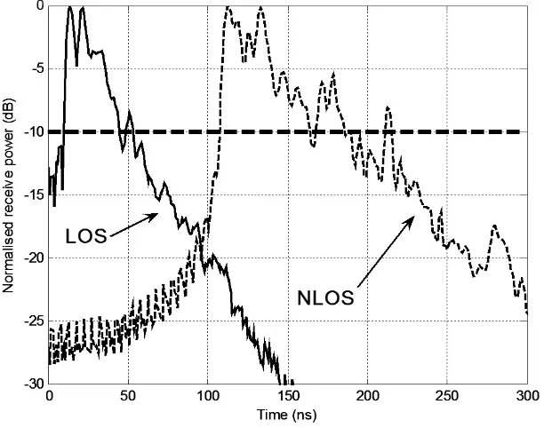
The Shannon capacity limit [1] demonstrates direct proportionality between capacity and received SNR. Multipath propagation results in both frequency and spatially selective fading, either of which readily degrades received signal strength. Figure 1 demonstrates that multipath fading could easily account for an SNR deficit of several orders of magnitude.
For example, (with the exclusion of any coding and modulation gains) a 30 dB fade could reduce SISO capacity by 9.97 bits/s/Hz. The potentially significant constraints on capacity and reliability of SISO systems in multipath propagation environments led to a need for research into the MIMO technique.
2.1.2 Multipath propagation conditions
Unimpeded propagation between transmitter and receiver is termed line of sight (LOS), while physical objects in the propagation path create non line of sight (NLOS) conditions. Figure 1 presents a comparison of measured SISO channels (using the apparatus described in chapter 3) for LOS and NLOS propagation environments.
Measurements were taken with the transmitter in the same room as the receiver for the LOS data and a different room for the NLOS case. The dominant main signal and moderate multipath (in this example due to furniture and other internal surfaces) characteristics of LOS transmission result in a comparatively high average power and lower number of deep fades. The presence of dividing walls and greater displacement between the transmitter and receiver are responsible for the loss of received power and increased incidence and magnitude of fades in the NLOS case.
2.1.3 Coherence bandwidth and time dispersion characteristics of multipath channels.
Received signals experience flat fading if the transmitted signal bandwidth is less than the coherence bandwidth (Bc) of the channel [29]; that is, the maximum
bandwidth for which gain is constant and phase is linear. In contrast, frequency selective fading results from a transmission bandwidth greater than the coherence bandwidth. All frequencies within Bc will exhibit correlated amplitude as they are
identically affected by the propagation channel. A pair of sinusoids with spectral separation greater than Bc
Figure 1 is likely to exhibit non-correlated amplitude or frequency selective fading. The full measurement bandwidth of 200 MHz depicted in is much greater than Bc for both LOS and NLOS examples, as frequency selective
For the case of the correlation function over time of two signals equal to or greater than 0.9, Bc may be approximated by [29]:
t c B
σ
50 1 ≈
A normalised power delay profile may be used to determine the rms delay spread, σt, commonly used to characterise the temporal behaviour of a wideband
multipath propagation channel. Rappaport [29] notes that a power delay profile is derived from an average of impulse response measurements in space or time taken in a given a local area. While Figure 1 demonstrates the frequency response behaviour of two distinct indoor propagation channels between a single transmitter-receiver pair, Figure 2 presents a normalised power delay profile, averaged over 260 channel realisations, for the same LOS and NLOS locations.
Figure 2: Measured power delay profile (normalised to 0 dB) for line of sight (LOS) and non line of sight (NLOS) propagation environments, showing -10 dB threshold used to calculate time
Several features of note are apparent in Figure 2: • Exponential decay is observed.
• Transmitter to receiver displacement is less in the LOS case.
• The intuitive expectation of greater delay spread arising from increased multipath is evident in the relative time dilation of the NLOS trace.
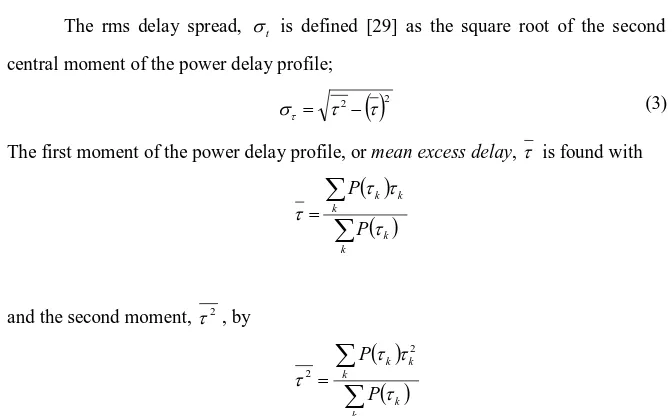
The rms delay spread, σt is defined [29] as the square root of the second
central moment of the power delay profile;
( )
2 2 ττ
στ = −
The first moment of the power delay profile, or mean excess delay, τ is found with
( )
( )
∑
∑
= k k k k k P P τ τ τ τand the second moment, τ2
, by
( )
( )
∑
∑
= k k k k k P P τ τ τ τ 2 2P(τk) refers to a multipath signal arriving τk after the first received peak at τ0
Time dispersion parameters calculated from
= 0. The total time multipath energy is received above a defined threshold (chosen to differentiate multipath components from thermal noise) is referred to as the maximum excess delay.
Figure 2 for a power threshold of -10 dB are shown in Table 1.
Table 1: Calculated time dispersion parameters relating to Figure 2
INDOOR CHANNEL TYPE LOS NLOS
MAXIMUM EXCESS DELAY (ns) 43 107
MEAN EXCESS DELAY (ns) 14.7 28.7
t
σ (ns) 9.9 22.9
Bc (KHz) 2020 873
Measured channel data demonstrate degradation in Bc as indoor channels
become NLOS, corresponding to an increase in multipath and received delay spread. Based on measurement results published in [29-31] and other sources, a delay spread of 200 ns is proposed as an approximate delineation between indoor and outdoor propagation channels in the upper UHF frequencies, with σindoor
Table 1 commonly below 50 ns in the references mentioned. The measured results presented in are thus in broad agreement with published data.
Both measured and published data suggest that traditional SISO communications systems tend to exhibit reduced capacity in the presence of multipath. Conversely, the alternative strategy of MIMO, with a demonstrated immunity to multipath, has generated immense interest.
2.2
Operating principles of MIMO Communication
systems
The MIMO method of data transmission evolved to combat the capacity limit and multipath sensitivity inherent in SISO. MIMO employs a combination of hardware and software to generate an increase in channel capacity (bits/s/Hz) over SISO systems and to confer immunity to multipath in rich scattering indoor and outdoor environments. Physically, a multiple element array with transceiver hardware for each element is deployed at both ends of a communication link, with issues such as modulation schemes, channel estimation and power allocation handled in software. The conventional format to describe the dimension of a MIMO system is nR x
nT, where nR is the number of receive and nT the number of transmit elements. An
extension to the standard nomenclature is introduced to clarify systems employing multiple polarisations discussed later in this work. The nR x nT format is retained,
with the number of polarisations greater than one shown in subscript. For example, 4 x 22 describes two dual-polarised transmit elements and four single polarised receive
elements.
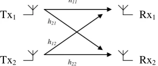
The most trivial manifestation of MIMO has four individual paths between transmitter and receiver. Figure 3 depicts the entries of a 2 x 2† channel response matrix, H, where hij represents the flat fading gain between transmit element j to
receive element i.
Figure 3: Schematic representation of a 2x2 MIMO channel representation
Uncorrelated entries in the channel response matrix are central to the operation of MIMO, permitting conveyance of separate and independent information sets from multiple transmit elements at the same frequency at the same time. As the entries of H become fully decorrelated, MIMO capacity approaches a potential maximum of min (nR,nT
To successfully decode incoming MIMO data in an actual system, the receiver must know the effect of the propagation channel on H, so a known preamble is sent on each transmit antenna. Incoming data is then decoded with this knowledge for as long as the channel is considered coherent. The receiver decodes the separate streams of information using one of a number of possible signal processing algorithms.
) x SISO capacity.
2.3
Cost / benefit considerations
Despite the proposed benefits, the implementation of MIMO systems may be impeded by greater cost, packaging and signal processing issues than for SISO. Generally, the use of an n x n MIMO system requires n separate transceiver chains, n
element arrays and suitable signal processing hardware and software at each end of the communication link.
In contrast, the significant capacity advantage and multipath immunity of MIMO may reasonably be expected to be of higher importance than the physical
† Equivalent systems with multiple polarisations are 1 x 1, 2 x 1 or 1 x 2.
h21
h12
h22 h11
Tx
1Rx
1packaging and financial costs of implementation in many cases. The preceding discussion has espoused the improvements to reliability of service and capacity for a given user with the adoption of MIMO architecture. MIMO may also be used to improve reliability of service for other users of the same band in the same local area. Transmit power, bandwidth or a combination of both could be reduced in a MIMO system to decrease interference between users, while still achieving or exceeding capacity identical to that of a SISO system.
2.4
Propagation model
Consider a multiple input multiple output communications channel, accessed by nR receive elements and nT transmit elements. The channel is assumed to exhibit
flat frequency fading, with packets short enough that any communication occurs within the coherence time, Tc
The complex baseband equivalent model of this system is given by [32]: of the channel. Equal power allocation is employed across all transmit elements and additive white Gaussian noise (AWGN) is the only additive signal at the receiver, as no more than one user transmits at any on time.
y = Hx + n
where x is the length nT transmit vector, y is the length nR receive vector, H is the nR
x nTcomplex channel matrix where hij represents the random i.i.d. fading between the
ith receive element and the jth transmit element and n is a length nR
2.5
Singular Value Decomposition
AWGN vector.
A common method of analysis of MIMO systems is Singular value decomposition (SVD) of the channel matrix. SVD generates k = min(nR,nT) singular
values, σ, which represent the voltage gains of the virtual SISO channels between the transmitter and receiver. SVD of H yields:
SVD(H) = UΣV†
(4)
where U and V are unitary matrices; nR x nR and nT x nT
†
in size, respectively. U and V are known as the left and right singular matrices. [.] is the conjugate transpose operator. Each of the k descending diagonal entries of Σ is an ordered singular value
of H, where Σ has the same dimension and rank as H. Matrix rank provides a measure of the maximum number of linearly independent columns or rows. The greatest achievable rank for a given matrix is equal to the smaller number of columns or rows. A matrix of full rank has completely independent entries, while a rank deficient matrix exhibits some degree of correlation.
With regards to MIMO, increasing decorrelation of the channel encourages full rank nR x nT
Considering
channel matrices. Correspondingly, the number of singular values and thus, sub channels, is maximised to the smaller number of transmit or receive elements with propagation channel decorrelation. The keyhole or pinhole effect is a notable exception to this generalisation; whereby uncorrelated channel transfer matrices exhibit low rank [18]. Diffraction around corners and waveguiding effects from propagation along hallways or narrow streets is one determinant of keyhole behaviour.
(4) and (5); decomposition of the channel matrix into independent sub-channels is achieved by filtering the transmitted and received signals with V and U†, respectively [32].
U†y = U†(HVx + n) U†y = U†(UΣV†Vx + n) U†y = Σx + U†n
Let y* = U’y and n* = U†n;
y* = Σx + n*
Figure 4 shows the application of (6), illustrating the decomposition of H into
k subchannels with gain, σ.
Figure 4: Subchannel decomposition of H
2.5.1 Sub channel redundancy
Consider an nT= 2, nR= 3 MIMO system as follows:
+ = * * * 0 0 0 0 * * * 3 2 1 2 1 2 1 3 2 1 n n n x x y y y σ σ
In the above case of nR > nT, y3 contains noise only. Similarly, for any MIMO
system where nT ≠ nR,, yz: z > k take no part in carrying data. However, techniques
such as choosing the best q x p system (where q < nRand p < nT
2.6
MIMO capacity
) from available array elements to exploit the extra spatial diversity available may be of benefit.
SNR [33]. Due to the non-trivial requirement for feedback of channel knowledge to the transmitter to undertake waterfilling, it will not be considered further.
With regards to the propagation model presented in Figure 3, the information theoretic, or upper bound on capacity, C (bits/s/Hz) for a complex AWGN MIMO channel under conditions of equal transmit power is: [2]
+ = † T 2 n det
log I
ρ
HHR
n C
where InR is an nR x nR identity matrix, ρ is the signal to noise ratio (SNR), nT is the
number of transmit antennas, H is the normalised (unit variance, zero mean) channel response matrix and (·)†
Calculation of capacity using
denotes conjugate transpose.
(7) requires the following assumptions:
• Propagation channel is sufficiently narrow band to be flat fading. Flat fading describes a channel where the signal bandwidth is less the minimum channel bandwidth that exhibits constant gain and linear phase.
• No channel knowledge exists at the transmitter. Under these conditions, the requirement for feedback is excluded and equal transmit power is applied across all transmit elements.
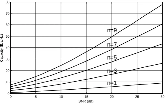
The capacity (bits/s/Hz) for n x n MIMO systems with increasing SNR is shown in Figure 5, clearly demonstrating the linear increase in capacity with the number of antenna elements [2]. The n = 1 case is equivalent to the Shannon limit, (1)
0 5 10 15 20 25 30 0 10 20 30 40 50 60 70 80 n=1 n=3 n=5 n=7 n=9 SNR (dB) C a p a c it y ( B /s /H z )
Figure 5: Capacity v SNR for various n x n MIMO systems
Received SNR is of critical importance to MIMO capacity. For example, consider a hypothetical 3 x 3 MIMO communication system transmitting with a 10 MHz bandwidth. With reference to Figure 5, the 1:1 gradient of the n = 3 case (for SNR greater than 12 dB) shows an additional 30 Mbits/s of capacity is achievable by doubling received signal power.
2.7
Normalisation
The usual objective of normalisation is to scale the entries of the channel response matrix to have zero mean and unit variance. The nR x nT x f channel
response matrix, H is normalised by division with the normalisation constant, η:
f n nR T n
i n
j f
k R T
⋅ ⋅
=
∑∑∑
2
H
η
SUMMARY
Chapter 2 has summarised the need for, and basic operation of multiple input multiple output communications systems. The behaviour of line of sight and
non line of sight propagation conditions has been compared through observation of measured data. The frequency response of a NLOS channel typically exhibits lower average receive power with a greater number of multipath induced fades. The increased complexity of multipath interactions, in conjunction with typically greater displacement between users increases delay spread in NLOS circumstances. The coherence bandwidth of measured channels decreases with transition from LOS to NLOS, although this may be alleviated with techniques such as the use of multiple sub-channels. The following topics are presented: a generic MIMO propagation model (with relevant assumptions regarding usage), singular value decomposition of a MIMO channel into the into min(nR,nT
3
) subchannels, equal power MIMO capacity and propagation channel normalisation techniques. A detailed discussion of the development and operation of the measurement system follows in Chapter .
Chapter 3
3 Chapter
H
ARDWARE
D
EVELOPMENT AND
O
PERATION
PREFACE
Chapter 3 consists of a discussion of the practical components to this project required to achieve the channel characterisation objectives listed in section 1.3,
The target accuracy for the measurements is –35 dB, sufficient for 4G wireless systems. The calibration method and precautions used to achieve this accuracy are also described in this chapter. The gathering of large quantities of propagation channel measurements necessitated the design and development of several items of automated transmitter and receiver hardware. Purpose specific software was written in the Labview development environment to undertake system automation and data gathering. Complete computer control of the measurement system allowed channel measurements to be taken late at night, free from human intervention and interference. Computer automation also relieves human operators of the drudgery of manual control while reducing the possibility of operator error affecting the data.
3.1
Development goals
Prior to commencement, several goals for this project were set under the global intention of channel measurement:
• To cost effectively and quickly develop a hardware solution to
characterise a typical indoor MIMO environment in the 2.4 to 2.5 GHz
ISM band, using omnidirectional, multiple element arrays. The measurement hardware is a multiplexed system using a single transmit element attached to a horizontally mounted x-y positioning system, with an RF-switch addressed, fixed receive array.
• Hardware and software to be readily reconfigured for other
measurement campaigns. Receive array composition is readily changed, as is the transmit element. The software allows alternative transmit-element locations and different inter-element separation on the x-y table to that used in the main measurement program.
• Hardware to have measurement accuracy commensurate with current-
any channel measurement data should be better than this to avoid dominating the performance of the link. A 6 dB margin is proposed, giving a channel accuracy requirement of -31 dB. Future uses of the measured data might require even greater accuracy and so the target accuracy for the equipment is set at –35 dB. This can be obtained if the accuracy of the three constituent parts of the measurement equipment, the mechanical sub-system, the electronics sub-system and the measurement SNR each meet an accuracy requirement of –40 dB (1%).
• To conduct further measurements with arrays of different composition
to the standard omnidirectional. Secondary measurement programs were undertaken. Data were gathered with directional receive elements or a dual polarised patch transmit element, using some of the original transmit locations. The use of several different antenna element types at the transmitter and receiver was intended to compare the performance of MIMO systems utilising various array structures.
3.2
Hardware description
The measurement system comprises a mobile transmitter, stationary receiver, network analyser and personal computer (Master PC) for system control and data storage. In the interests of minimising temporal and fiscal expenditure, the channel measurement hardware was developed as a multiplexed system, sequentially measuring each hij
The network analyser transmits a swept carrier from 2.3 GHz to 2.5 GHz and returns the complex transfer function of h
individually. The desirable alternative of sampling the full MIMO channel response instantaneously represented an unacceptable increase in hardware development cost and time.
ij
Figure 6
Figure 6: Measurement apparatus showing connection to the Network Analyser (NA). Dark lines show the RF signal paths.
The Master PC controls the movement of the antenna at the transmitter and the action of the RF switch at the receive array, in addition to controlling the operation of and storing data from the network analyser. At a given transmit table location, the x-y positioning system moves the transmit element to the first selected position. From the transmit element, the network analyser measures nR complex frequency responses,
multiplexing each receive array element with an RF switch. The transmit element is moved to any subsequent locations before the channel is sampled again to each receive element; fully characterising the nR x nT
GPIB
3.2.1 Receiver
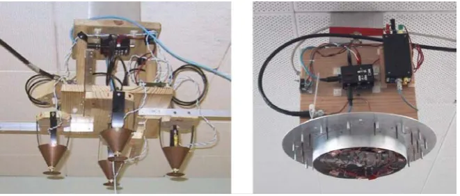
Figure 6 schematically shows an n element receive array (n = four or eight, for the omnidirectional and directional arrays, respectively) with associated low noise amplifiers and RF switch. The directional and omnidirectional receive arrays were used in separate measurement campaigns. Figure 7 shows that the omnidirectional array utilises four discone antennas, while the directional array employs eight dipoles.
Figure 7: Four-element omnidirectional (left) and eight-element directional (right) receive arrays as installed to a laboratory ceiling.
The receive arrays were co-located to the same point on the ceiling of a laboratory at a height of 2.3m for each measurement campaign. The basic structure of either array is an RF switch multiplexing the amplified signal from each antenna to the network analyser.
Omnidirectional receive array
Figure 8: Block diagram of the omnidirectional array. With the exception of the discone antennas, labelled components are common to directional array also. Antenna and associated LNA location is adjustable to any of three locations, providing adjacent antenna displacement of
one, two or four λ at 2.45 GHz
Directional receive array
The directional array is an eight-sector antenna. Eight dipole pairs tuned to 2.45 GHz are arranged circularly in the horizontal plane. The antenna elements are arranged with a radial distance of 150 mm, in front of an annular reflector of radius 120 mm (Figure 7 right). Each dipole element has a director element in front of it. As with the omnidirectional array, a network analyser samples received signals through a low noise amplifier and RF switch arrangement. The directional array structure (excluding low noise amplifiers and RF switch) was kindly provided by Stewart Jenvey of Monash University.
3.2.2 Ancillary Receive array hardware
Power supply
The power supply consists of a sealed lead-acid battery and LM78XX series linear regulators [34], supplying voltage to the RF switch, switch controller and low noise amplifiers. The use of a battery in place of a leaded power supply avoids complicating factors such as ground loops and RF noise being coupled into the receivers through a long power lead.
RF switch
A SP8T RF switch is used at the receive array to multiplex the amplified signal from each receive array element to the network analyser (See Figure 6). 50Ω loads occupy the four unused ports when used on the four element omnidirectional array.
The RF switch is composed of a Hittite HMC284MS8G SPDT switch multiplexing a pair of Hittite HMC241QS16 SP4T switches, thus providing the SP8T functionality required for use with the directional array (see Schematic 2 of Appendix A). The four-into-two arrangement ensures better insertion loss and greater overall isolation between ports than for a Hittite HMC253QS24 SP8T switch alone. Figure 9 shows the measured insertion loss and leakage characteristics.
Figure 9: Typical RF switch insertion loss and leakage
The RF switch controller governs the operation of and powers the RF switch. Each of the three devices in the RF switch uses two control lines to determine switch position.
RF switch controller
An RF switch controller interfaces the parallel port of the Master PC to the RF switch. The switch controller is a generic device, able to operate RF switches in SP4T, SP8T or SP16T modes (see Schematic 3 of Appendix A). Switch banks A, B and C are three RF switch control ports. Banks A and B have drive capability for a SP8T switch, while bank C drives a SPDT switch. Control of SP4T and SP8T switches is available from bank A, while full SP16T functionality is realised when a SPDT switch on bank C multiplexes SP8T switches on banks A and B.
A three-way toggle switch determines the four, eight or sixteen throw mode of operation, with RF switch position and active RF switch bank shown on seven-segment displays. The first character displays A or B while the second shows the current RF switch position for that bank.
IN input port increments the RF switch position by one. A reset action initialises the switch position when in clock mode.
The parallel input mode sets the RF switch position to reflect the first four bits of the parallel port connected to the controller. In parallel mode, the lower three bits of the input data nibble determine the switch position (1 to 8) and the MSB sets the active bank. For example, the nibble ‘0111’ would specify bank A, position 8. A reset action will not be apparent in parallel mode if data remains at the input. In this case, the device will immediately return to the value stipulated by the input before the application of reset.
In the case of this work, the parallel port of the Master PC determined the position of a SP8T RF switch attached to bank A of the RF switch controller.
Low noise amplifiers
The low noise amplifiers are based on the Minicircuits ERA-3SM monolithic amplifiers [36] with a noise figure of 2.9 dB @ 3 GHz. This device is small, easy to implement, of low cost and has relatively low noise (see Schematic 4). Blocking capacitors at the input and output of the ERA-3SM isolate the DC supply and RF signal paths; a capacitance of 12 pF achieves a target series impedance of 5 Ω at 2.45 GHz. The Darlington pair configuration of the ERA-3SM requires a constant current source for stable gain, approximated by the series bias resistance. A parallel combination creates the desired resistance with reduced heat dissipation per resistor.
The 7 v supply allows some headroom with dropping battery voltage. With a 2.5 v drop across the linear regulator, a fully charged battery of 13.8 v can drop 4.3 v before the low noise amplifiers are affected. A relatively low bias voltage also assists further with heat dissipation in the bias resistance.
3.2.3 Transmitter
While a multiplexed transmit array could have been implemented in an identical manner to that at the receiver, a synthetic array generated with a single mobile element was chosen. The synthetic array possesses two significant attributes; excellent user definability and potentially large array size without complicated RF switching networks.
The dual axis antenna positioning system, or x-y table uses a rack and pinion drive system to horizontally locate the transmit antenna with a resolution of 0.1 mm. Software on the Master PC controls the antenna location on a 17 x 17 grid where the inter-positional spacing is usually predefined at 30.6 mm (corresponding to λ/4 at 2.45 GHz). The x-y table is mounted to a mobile cabinet housing a dual stepper motor controller, RF power amplifier, laboratory power supply and a personal computer (Slave PC) as shown in Figure 10.
Figure 10: The transmit x-y table
The central item of hardware on the transmitter is the dual stepper motor controller, developed to accomplish the following tasks:
Discone transmit antenna
Power amplifier
Stepper motors
Dual stepper motor controller
• To move the transmit antenna by controlling a stepper motor for each of two
horizontal axes.
• To switch supply voltage to the power amplifier and an optional pre amplifier. The pre amplifier is occasionally necessary to ensure good SNR with long transmission distances.
• To control a 2-way RF switch for use with a dual polarised antenna or a
two-element array.
The Slave PC in this installation is simply an interface between the dual stepper motor controller and the local area network (LAN) connection to the Master PC. Neither parallel nor RS-232 serial links are reliable over the potentially long distances between transmitter and receiver required for this project. Unlike other potentially faster methods, a LAN link posed a minimal time and financial burden to implement. The dual stepper motor controller decodes serial control information sent by the Slave PC to drive the two stepper-motors, one for each horizontal axis.
The dual stepper motor controller also receives data from the first two bits of the Slave PC parallel port to control relays used to switch 12 V to the power amplifier and optional preamplifier. A MAX232 serial transceiver converts RS232 line levels from the Slave PC into TTL levels for a PIC16F84 micro-controller. The PIC provides control and distance counter signals to each motor controller block. These consist of an L297 stepper motor controller driving an L298 H-bridge stepper motor driver.
cycles. Alternatively, a more common technique such as an 8-bit CRC could have been employed.
Displacement accuracy
In the case of measured data generated by the hardware described in this thesis, EVM is exacerbated by phase errors arising from inaccurate transmit element positioning. In the interests of maximising data quality, an EVM of -40 dB was desired in the measured data, corresponding to a phase error of 0.01 radians or a displacement error of 0.0016 λ. A 2.45 GHz carrier has a wavelength of 122.45 mm, so the x-y table should ideally exhibit positional resolution of 0.196 mm or better. The stepper motors are 1.8°, 200 step units that in conjunction with a drive pinion of diameter 37.8 mm, result in 648 clocks/λ (at 2.45 GHz). This equates to 0.189 mm of antenna travel per output clock (in full step mode) and is equivalent to an EVM of -40.3 dB. With the speed set to half step mode, this resolution increases to 0.094 mm/clock. Both full and half step modes have sufficient resolution to achieve the desired positional accuracy.
3.2.4 Network Analyser
3.2.5 Master PC
The Master PC automates the operation of the entire measurement apparatus and saves the results of any measurement data from the network analyser. Software written for this work governs the time of the first measurement, controls all relevant network analyser settings, selects the current RF switch position and determines all actions of the transmit table. The Master PC is linked to the network analyser with a GP-IB interface, to the RF switch with a parallel cable and to the Slave PC with the local area network.
3.2.6 Measurement Software
A purpose-programmed virtual instrument (VI) within the Labview
development environment automates the measurement system. The operator is presented with a graphical user interface as shown in Figure 11, which allows control of transmit antenna locations, number of RF switch ports and network analyser measurement parameters.
The VI also provides a checklist of tasks to ensure correct initialisation of the hardware, reducing the risk of erroneous data due to operator error. A time and date delay feature allows early morning measurements to ensure a static channel, free from human interference. Additionally, thermal equilibrium of the transmit power amplifier is assured prior to data gathering with a pre-measurement warm up period.
The user can select any number of transmit antenna positions up to 289, from a 17 x 17 grid. At a software level, the contents of each column of the input grid are examined sequentially for selected transmit antenna locations. This results in the transmit antenna moving in a scanning pattern over the possible range of movement. In response to one or more positions in column A, the antenna will move along the vertical axis to these sequentially, before moving back to the horizontal axis after measurement at the last location in the column. Movement is then initiated in the horizontal axis to the next column (B to Q) containing a transmit position so that a vertical cycle can be repeated. This regimen ensures that desired movement in each axis occurs in one direction only; the vertical axis is reset to a home position for each new column. The direct benefit is that backlash in the stepper motor drive pinion relative to the rack is avoided by not making repeated movements back and forth without mechanically resetting to a known position.
While the software allows for up to 289 user-definable transmit antenna locations, measurements with the omnidirectional receive array used a preset star pattern of 65 locations. The number of transmit element locations was reduced to 33 for directional array measurements to reduce the overall measurement time for a given table location.
The most important user defined settings of the VI are as follows:
• Checklist. The top left corner of the VI has a frame containing a text message and a CONTINUE button. Measurement will not begin until a series of initialisation steps have been carried out to reduce the possibility of a set-up error rendering a data set useless. The user is stepped through the initialisation process, ensuring each item of hardware is connected and calibrated as necessary to guarantee correct system function.
entered here. There is no hardware requirement to limit this distance to λ/4 since the number of cycles per movement is user definable. The minimum movement corresponding to one cycle is 0.094mm (or 8.36x10⁻⁴
• Measurement type. Channel measurements are taken with the default GATHER DATA setting, while CALIBRATION is used to measure the hardware frequency response alone. The application of hardware calibration data to a measured channel response isolates the actual channel response from the measured data that also includes hardware influences. Refer to section
λ @
2.45GHz), for the benefit of any future use of the hardware.
3.5.1 for full description of this process.
• Save to file. While enabled by default, file saving is an optional function to facilitate error checking and system demonstrations.
• Time to begin measurement. Allows date delay and time delay to start of measurements.
• Transmit table details. This is a pull-down menu of transmit table locations, listing the IP configurations for network ports near each table location.
A test run measurement is taken at the end of the set-up process, allowing confirmation that a channel measurement has in fact been taken and saved to the correct location with the correct naming convention. The gain and phase responses of the propagation channel between a given transmit element location and each receive antenna is displayed for demonstration and error checking purposes.
Data storage
DirectionalRm1Pos1_tx@E4_8ant and Rm1Pos1Rxa_tx@A0_4ant are examples of saved file names.
3.2.7 Antenna development
This work utilised a combination of purpose developed and externally sourced antennas, all based around conventional designs. The discone and dual polarised patch antennas were developed as part of this work, while a colleague donated the circular dipole array.
Discone
The discone topology has the beneficial characteristics of very wide bandwidth, omni-directionality, modest cost and simplicity of fabrication. The discone antenna developed for this work and corresponding radiation pattern is presented in Figure 12.
Figure 12: Discone antenna and measured vertical radiation pattern
Scattering parameters were measured for this design on the HP8753C network analyser, revealing an exceptionally wide –10 dB bandwidth from 1.04 GHz to beyond 6 GHz (the upper frequency limit of the machine), ensuring a flat frequency response in the band of interest. The cone was formed over a mandrel while spinning on a lathe from a flat disc of 0.5 mm copper, with the apex dimensions to suit an N-type RF connector (Huber + Suhner part number 22_N-50-0-2/133_N). Figure 13, with dimensions in mm, shows this was utilised as it forms part of the structure by joining the cone and top disc together, in addition to providing electrical connection. A copper rod soldered to the centre conductor of the N connector facilitates tuning, where the top-to-cone clearance is adjusted for optimal standing wave ratio on the network analyser. The dimensions shown were found to provide good (-20 dB) matching at 2.45 GHz in addition to the previously mentioned wide bandwidth.
Figure 13: Discone element cross-section
Development of the discone dimensions was an iterative process, beginning with the following initial approximations:
Disc diameter: 0.17 λ Cone side length: 0.25 λ
Cone apex angle: 25º - 40º, 30º used
above call for disc diameter and cone length to be 51 mm and 75 mm, respectively. Trial and error while observing standing wave ratio on a network analyser resulted in the final dimensions shown in Figure 13.
Circular dipole (directional) array
The circular dipole or directional array represents the type of installation that may be more typically employed as a directional, multiple element base station array in a wireless communication system. The measured radiation pattern of the circular dipole array in the horizontal plane, Figure 14, indicates the directionality of one element.
Figure 14: Radiation pattern of a single sector from the eight sector directional array (Figure 7 right)
The standard measurement bandwidth of 200 MHz is restricted to the operational bandwidth of 85 MHz for data analysis of MIMO systems using the directional array. The circular dipole array used the same power supply, RF switch, switch controller and low noise amplifiers as the omnidirectional array.
charts the mean return loss over all eight elements of the dipole array, while the dotted trace presents the worst case (adjacent element) cross coupling between dipole array elements to be an average of –31 dB over the operational bandwidth. Typical cross coupling between non-adjacent elements is –50 dB.
Figure 15: Mean return loss and worst case inter-element cross coupling of dipole array (Figure 7right)
Dual polarised patch
r L
c f
ε
2 ≅
where c, L and εr
Strategies for array miniaturisation were examined in this work, including reducing individual element and overall array size. Equation
are the speed of light, length of patch and relative permittivity of the substrate, respectively.
(7) indicates that increasing εr
Accuracy, ease of and rapidity of manufacture were paramount for the measurement programs described in this project. A microstrip antenna made by machine, solely from readily available PCB substrates was more desirable than one requiring time-consuming sectional assembly.
is a viable approach to reduce the resonant length of the patch. Another common technique is the use of an edge-shorted half wave patch, creating a quarter-wavelength device with a 50% reduction in physical length. Inducing meandering surface currents of an excited microstrip antenna is another well-known and simple method of lowering the resonant frequency; or reducing patch size for a given frequency. Cutting notches of appropriate dimension and location into the edges or body of a patch increases the minimum surface current path length.
Applying any of the above techniques to individual array elements may reduce overall array dimensions, but reducing the actual number of physical devices is also of benefit. A dual-polarised structure with sufficient isolation between polarisations would halve the number of antenna elements, potentially very useful in volume critical applications such as hand-held devices. An existing design [37] for operation at 1870 MHz was adapted to 2.45 GHz for this work as it had several desirable characteristics. It is a mass-producible design based upon a common PCB material (FR4), requiring no further construction work postproduction than simply installing connectors. Figure 16 shows the dual polarised patch antenna used for this work.
The patch is fabricated from double-sided board with a ground plane on the reverse side. The outer edges of Figure 16 indicate the ground plane perimeter (refer to appendix C for dimensions) relative to the patch dimensions. This device is probe fed, as evidenced by the two regions of solder near the centre of the patch. Two short lengths of semi-rigid cable terminated with SMA connectors are soldered to the ground plane, with the centre conductor passing through the board to excite the patch.
The combination and arrangement of slots in the surface of the patch results in 16.8% miniaturisation from the length of 29.19 mm for fc
(7)
= 2.45 GHz, calculated with . Figure 17 shows the frequency response of the dual polarised patch used in this work. The solid trace of Figure 17 shows the antenna input matching, while the dotted line is the cross polarisation leakage. The -10 dB bandwidth of the dual polarised patch antenna is 53 MHz, centred at 2.452 GHz. The mean cross polarisation leakage over the operational bandwidth is –25 dB.
3.3
Measurement programs
Following completion of the hardware, measurements commenced in January 2002. Three measurement programs were undertaken on the seventh floor of building D and the Footscray Park campus of Victoria University in Melbourne. The complete propagation measurement database created for this project comprises information from a primary and two secondary measurement programs. Each of the three campaigns occurred in the same propagation environment. Table 2 outlines the various transmit and receive architectures used in the three measurement programs.
Table 2: Measurement program details
Program Transmit element Receive array Comments
A Discone Omni Primary data set
B Discone Directional Reduced Tx locations
C Dual polarised Patch Directional One Tx location only
Program A included 23 individual transmit sites throughout the building, extensively characterising the propagation environment under a wide variety of line of sight (LOS) and non line of site (NLOS) conditions. Program A represents the main body of the measurement effort and constitutes a baseline for alternative hardware comparisons.
Program B was essentially identical to program A, with the exception of the receive array and was intended to allow investigation of any potential difference between directional and omnidirectional receive arrays.
Program C sought information about a more realistic choice of transmit antenna topology than the bulky discone type.
laboratories and a hallway, chosen to include a combination of LOS and NLOS scenarios.
LEGEND
Receive array, either omnidirectional or directional.
O Omnidirectional transmit array with omnidirectional receive array. + Omnidirectional transmit array with directional receive arrays.
Dual-polarised transmit array with directional receive array, in addition to the ⊕ combination.
Figure 18: Building D, Level 7 - Victoria University Footscray Park campus.
3.4
Measurement protocols
An optical plummet1
The ability to accurately reposition the transmitter table between measurement programs or in the event of a table disturbance during a program governed decisions on transmitter placement. This required unobstructed access to fixed reference points, usually a wall or other immobile object, from which the optical alignment device could be employed.
was adapted for use in the horizontal plane and allowed the transmitter to be repositioned with a very high degree of confidence between measurement programs. The optical plummet allowed small registration marks on adjacent walls to be telescopically observed while making fine adjustments to the transmitter location, ensuring accurate replacement of the hardware between measurement campaigns.
3.5
Data quality
Several initiatives aimed to ensure the highest possible quality of measured data: in the interests of aiming for the –40 dB accuracy of the mechanical subsystem, electrical subsystem and measured SNR mentioned in section 3.1
• Regular network analyser calibration. Factors such as ambient temperature and physical orientation affect the frequency response of the RF cables used to connect the network analyser to the transmitter and receive array. Calibration of the network analyser cabling occurs at the network analyser prior to the gathering of data at each transmitter location.
• Power amp warm up. Turning the power amplifier on 30 minutes before measurements commence ensures thermal equilibrium of the device.
• Transmit table location accuracy. The use of an optical plummet as described in section 3.4 allowed sub millimetre horizontal accuracy of the transmit table.
• Transmit element location accuracy. While the optical plummet provided precise spatial positioning for the array as a whole, relative
1
spatial positioning accuracy between transmit array elements is of greater importance. The horizontal positioning system (section 3.2.3) accuracy is equivalent to -40.3 dB in full step mode or -46.3 dB in half step mode; both in excess of the -40 dB design goal.
• Double shielded RF cable. Cable leakage was minimised by the use of Huber + Suhner RG 214/U-01 double shielded cable, reducing the likelihood of direct coupling between the RF cabling attached to the network analyser.
• Human and RF interference reduction. Late night measurement times significantly reduce the likelihood of external interference from pedestrian traffic or other RF sources
• Hardware calibration. The application of ancillary hardware frequency response to measured data isolates the propagation channel from measured data, which includes influences from the electronic sub-system. This is described in detail in section 3.5.1.
3.5.1 Hardware Calibration
The ultimate goal of any measurement program is to produce data that accurately represents the channel response only and not a combination of the channel and measurement hardware. Hardware calibration measures were developed by observing the following frequency response representation of the measured channel response, H◊:
H◊ = L . α . H . g
where L is nR x nR the insertion loss and leakage matrix of RF switch, α is an nR x 1
frequency response vector of the low noise amplifiers, H is the nR x nT
Since the transmit array of this system is synthetically generated with a single antenna and power amplifier, g is in fact a scalar and may be grouped with the receive hardware resulting in a single term, χ, representing all non-channel based artefacts.
actual channel response matrix and g is the transmit power amplifier response vector.