An Edge-detection and HPF Based Intelligent Space - A Network Based Integrated Navigation System.

(1)

ABSTRACT

GUPTA RACHANA ASHOK. An Edge-detection and HPF based Intelligent Space – A Network

Based Integrated Navigation System. (Under the direction of Dr. Mo-Yuen Chow.)

Intelligent space (iSpace) is a large scale mechatronics system. It is a multidisciplinary

effort whose aim is to produce a network structure and components that are capable of integrating

sensors, actuators, DSP, communication, and control algorithms in a manner that suits

time-sensitive applications including real-time navigation and/or obstacle avoidance. There are many

challenges that must be overcome in order to put such a distributed, heterogeneous system together.

The research presented here deals with one of these issues, i.e. the adverse effect of processing

delays on the system. Here a novel structure for a delay-resistant sensory-motor module to

navigate a differential drive unmanned ground vehicle (UGV) in a cluttered environment is

suggested. The module consists of an early vision edge detection stage, a harmonic potential field

(HPF) planner; a network based quadratic curve fitting controller and gain schedule middleware

(GSM). The structure of this module and its components are described. Thorough experimental

results along with performance assessment comparing to the previous implementation are also

(2)

A

N

E

DGE

-

DETECTION AND

HPF

BASED

I

NTELLIGENT

S

PACE

–

A

N

ETWORK

B

ASED

I

NTEGRATED

N

AVIGATION

S

YSTEM

by

RACHANA ASHOK GUPTA

A thesis submitted to the Graduate Faculty of North Carolina State University

in partial fulfillment of the requirements for the Degree of

Master of Science

ELECTRICAL ENGINEERING

Raleigh, North Carolina

May 2006

APPROVED BY:

______________________ _____________________ Dr. Wesley Snyder Dr. James J. Brickley

(3)

To my parents, and my sister Apeksha

who taught me that

(4)

BIOGRAPHY

Rachana Ashok Gupta was born in Tarapur, India on the 22nd of January 1981. She

received her Bachelor of Engineering degree in Electronics and Telecommunication engineering in

2002 from Maharashtra Institute of Technology, University of Pune, India.

She worked as an Associate Consultant and Software Engineer in iFlex Solutions Ltd,

Mumbai, India in development and testing of banking software for the period of September 2002 –

July 2004.

Later in fall 2004, she joined Master of Science program in the Department of Electrical

and Computer Engineering of North Carolina State University, Raleigh. She became a part of

Advanced Diagnosis Automation and Control (ADAC) lab directed by Dr. Mo-Yuen Chow in

spring 2005. Her main research interests are computer vision for network based robotics,

computational intelligence and mechatronics systems. Her current research topic is network based

integrated navigation systems for unmanned ground vehicles. With the defense of this thesis, she is

(5)

ACKNOWLEDGEMENTS

I cannot thank enough Dr. Mo-Yuen Chow, who taught me the real meaning of the two lines which always inspired me:

Some people see things as they are and say why??? I see things those never were and say why not!!!

His invaluable guidance, great encouragement, persistent support and faith in me during the course of this research were my greatest motivators. He not only created immense opportunities for me to build up my knowledge, confidence and research capabilities but also shaped my philosophy in science and research.

I am highly grateful to Dr. Ahmad Masoud, King Fahd University of Petroleum and Minerals, Saudi Arabia. His immense knowledge, guidance, suggestions and persistence have a great share in successfully completing the research presented in this thesis.

I would like to express my sincere appreciation to my committee members: Dr. James Brickley for the continuous encouragement and faith in me, Dr. Wesley Snyder for the invaluable discussions and suggestions during and outside the teaching of the course of Computer Vision, which built the foundation of my research in computer vision for robotics.

I would also like to acknowledge the help from the members in ADAC lab: Rangsarit Vanijjirattikhan, Puxuan Dong, Le Xu, Zheng Li, Tyler Richards, Tao Hong, and Manas Talukdar. I have benefited enormously from the inspiring academic atmosphere in the ADAC lab.

My special thanks go to the electronic lab staff member Rudy Salas for his help in hardware facilities.

Of course, none of this would have been possible without my parents, their unconditional love, support and the struggle they have gone through in life to ensure my continuous progress that I have been able to strive so hard to succeed in every venture of my life and reach these academic heights. My sister Apeksha, who is my moral support system, has always been an enthusiasm for my studies.

(6)

LIST OF TABLES

Table 1: Sampling ticks with Δs = 1 to form 7x7 approximated kernel for ∂G(σ,x,y)/∂x and

y y x

G ∂

∂ (σ, , )/ at σ = 1 ... 23

Table 2: Calculations for Template matching computations ... 37

(9)

LIST OF FIGURES

Figure 2: iSpace block diagram ... 5

Figure 3: The graphical user interface on the internet ... 6

Figure 4: iSpace workspace image and templates for Template matching... 9

Figure 5: Finding the orientation of the UGV. ... 9

Figure 6: Explaining the restrictive assumptions by template matching about the size of the obstacles... 11

Figure 7: Path planning in iSpace ... 12

Figure 8: Sequence of path generation with fast marching method... 12

Figure 9: Path planning using fast marching method avoiding the obstacles... 13

Figure 10: Path tracking control using quadratic curve ... 13

Figure 11: Figure explaining the disadvantage of going for a fixed reference path ... 15

Figure 13: 3-D plot of 2 ( , , )at σ = 1 ... 18

y x G σ ∇ Figure 14: 2 ( , )versus r with σ = 1... 18

r G σ ∇ Figure 15: workspace image I and its zero crossing contour for _I_{⊗ ∇}2_G ... 21

Figure 16: 2-D Gaussian curveG(σ,x,y) ... 21

Figure 17: Complete edge detector block diagram ... 22

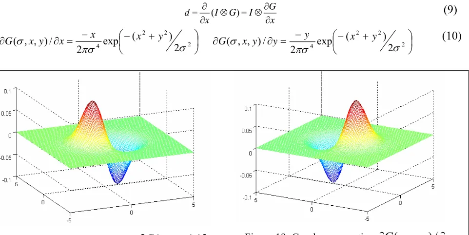
Figure 18: Graph representing∂G(

σ

,x,y)/∂x... 22

Figure 19: Graph representing ∂G(σ,x,y)/∂y ... 22

Figure 20: Cross-section of the ∂G(σ,x,y)/∂xat a plane y = 0 with σ = 1... 24

Figure 21: A 20x scaled 7 point approximation of ∂G(1,x,0)/∂x... 24

(10)

Figure 23: A 20x scaled 49(7x7) point approximation of ∂G(1,x,y)/∂x... 25

Figure 24: Top view images I(x, y) with their corresponding edge maps E(x, y)... 26

Figure 25: HPF results with synthetic edge maps... 30

Figure 26: Figures showing the result of HPF planner – Region to Point guidance function. ... 31

Figure 27: HPF gradient image enlarged explaining the concept of discrete look-ahead distance. 33 Figure 28: iSpace workspace images showing the effect of different values of look-ahead distance chosen ... 33

Figure 29: Distance error increases and total time to reach the goal decreases with increase in δL. ... 34

Figure 30: Template matching and Edge detection outputs for the same workspace image... 37

Figure 31: Behavioral comparison between “path tracking” and “goal seeking” problem ... 40

Figure 32.Complete flow diagram of the new system. ... 43

Figure 33: Actual workspace images and the graph of distance error as a function of time. ... 45

Figure 34: Actual Network delay... 46

Figure 35: Mean Median and Max distance error as a function network delay for HPF planner. .. 47

Figure 36: Left – HPF planner and Right – fast marching planner for same grid size... 47

Figure 37: Maximum and mean distance error vs. network delay comparing fast marching and HPF planner... 47

Figure 38: Total time vs. network delay comparing fast marching and HPF. ... 48

Figure 39: Navigation results with network delay = 1.1 s and look-ahead distance = 0.4 m. ... 48

(11)

CHAPTER I

– Introduction

For many years now, data networking technologies have been widely applied in the control of

industrial and military applications [1]. These applications include manufacturing plants,

automobiles, and aircrafts. Connecting the control system components in these applications, such

as sensors, controllers, and actuators, via a network can effectively reduce the complexity of the

systems with nominal economical investments. Furthermore, the applications connected through a

network can be remotely controlled from a long-distance source. A Network based Integrated

Navigation System presented here is one subset of the whole genre of Network Based Systems. It

has different modules combined together to guide a UGV (Unmanned Ground Vehicle) from one

point to another in the space of interest (ℜ2_{), where the navigational intelligence lies on a main}

controller away from the UGV. Having a remotely controlled integrated navigation system; where

the data processing, and controller module are at a central location (network controller) driving all

the UGVs has many different advantages over a system with autonomous UGVs. Network

controllers allow data to be efficiently shared. It is easy to fuse the global information to take

intelligent decisions over a large physical space. It is easy to add more sensors and UGVs with

very little cost and without heavy structural changes to the whole system. And most importantly,

they connect cyber space to physical space making task execution from a distance easily accessible

(a form of tele-presence). These systems are becoming more realizable today and have a lot of

potential applications such as manufacturing plant monitoring, nursing homes or hospitals and

tele-robotics & tele-operation etc. Fusing the global information to make intelligent decisions or to

perform a particular task requires integration of different modules like data acquisition, data

(12)

independently yet together making it one system. Therefore, a few of the issues faced by a network

based navigation systems are network delay, processing delay, data sharing and data transfer. Thus

it is evident that to improve the efficiency of a network based integrated system; we not only have

to improve each integrated module but also focus on the efficient data interface between different

modules. This is one of the main points of emphasis in the research presented here.

We deal with a prototype of Intelligent Space (iSpace) as a network based integrated

navigation system as the research platform here. iSpace in ADAC lab at North Carolina State

University is a closed-loop system consisting of different modules like image processing,

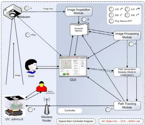
automation control, communication and networking for navigation of a differential drive UGV in a

2-D space of interest (ℜ2_{) as shown (Figure 1). Currently, iSpace in ADAC lab is implemented}

using three basic modules: (i) A template matching-based vision system to recognize the contents

of the environment, the UGV and their configurations [42] (ii) A planning module for computing

the optimal, obstacle-free, reference path for the UGV using the fast marching method (gradient

decent algorithm) [45] [44] (iii) A quadratic curve fitting path tracking module that uses the

sequence of control commands generated by the main network controller after compensating for

time delay in the closed-loop navigational system [37][41]. There are several challenges facing the

reliable operation of the above system. Different delays are the main issues related to any

network-based integrated control system. In iSpace, delays such as

1. Network (data flow) delay – Image data from camera to the controller, Command data from

controller to robot.

2. Processing or computational delay – Image processing using template matching, Path

(13)

restricted to a specific case of environment, where all the obstacles in the workspace need to have

a pre-decided template on them. This restricts the workspace flexibility. Once the path is generated

using fast marching method, the problem is converted to a path tracking problem. Therefore, the

same path has to be tracked irrespective of how far off the UGV wanders away from that reference

path in the due course of movement because of the network delay. This may not be always an

intelligent decision considering path and time optimality.

Figure 1: Structural flow diagram for iSpace

We mainly focus on the image processing and the path planning part of the integrated

navigation system to develop a more efficient, more generic structure for iSpace in ADAC lab.

Instead of template matching, we use edge detection to extract the contents of the workspace. This

helps the system to be more generic in terms of obstacle map. Edge detection is also more efficient

in computational complexity than template matching. We also replace the Fast marching method

by Harmonic Potential field (HPF) [3][7] to generate the guidance directions for path planning.

(14)

problem; so UGV can be driven to the chosen goal from any point in the workspace, which also

makes it compatible with the network based controller giving the effect of smaller real time

computational delay. Although the marriage between the edge detection and HPF-based planner as

well as the marriage between HPF based planner and the quadratic path tracking controller are the

only modules in an interconnected structure, they simultaneously satisfy several important features

that are central to the integration of the system. Here we emphasize on the compatibility between

the different modules of the new system. This compatibility makes it possible for a module to

directly accept the output from another module without any conditioning required, hence

significantly reducing the processing delay and the chance of inter-module conflict. We believe

that creating a homogenous structure by putting edge detection, HPF planner and quadratic curve

fitting path tracking controller - three heterogeneous systems together for the first time to create a

network based system is the novel contribution to the network based integrated navigation system

area. These features and ones possessed by the other modules are discussed in later chapters

elaborating the advantages in the quantifiable performance measure. We believe that these criteria

are the key to building a system that will behave in the desired manner. Chapter II talks about the

functional and algorithmic details of the system under consideration – iSpace – as a network based

integrated navigation system, the features and functionalities of different integrated modules,

disadvantages and restrictions of the current system, and scope of improvement. Chapter III

explains the new structure and the component details. Chapter IV elaborates its advantages over

the previous structure as individual modules as well as the successful integration of the complete

system and advantages over the previous integrated system and eventually the enhancements

accomplished as a delay tolerant structure of network based integrated navigation system. Finally,

(15)

CHAPTER II

– Introduction to iSpace as a

Network based Integrated Navigation system

The network based integrated navigation system considered as a research platform – iSpace –

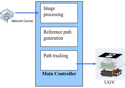
[42] has the following components (as shown in Figure 1 and Figure 2):

2. 1

Different components in iSpace

UGV

Image processing

Reference path generation

Path tracking

Main Controller

Figure 2: iSpace block diagram

(i) An overhead network camera is used as a global sensor. The web camera collects the

top-view image of the 2-D space of interest and sends to the main controller for processing.

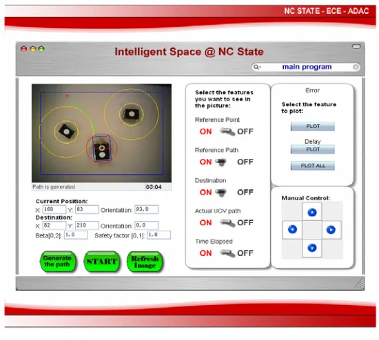
(ii) Network controller with graphical user interface (GUI) (Figure 3), which can be on any

remote computing interface in the world having the access to internet. The main network

controller is connected to the global sensor – network camera and the actuator – the UGV –

in the space of interest through a wireless channel. All the functional modules and

(16)

space from the network camera and take the decision to be conveyed to the UGV in the

space in the form of a mobility command. (Figure 2). All the algorithms on the main

controller are explained in detail further in Chapter II.

Figure 3: The graphical user interface on the internet

(iii) A differential drive UGV is the actuator / navigator in iSpace.

1

2 1

2 W

r r

W

r r

r

l

ω _ν

ω = − ω

⎛ ⎞

⎛ ⎞ _{⎛ ⎞}

⎜ ⎟

⎜ ⎟ _{⎜ ⎟}

⎜ ⎟ ⎜ _{⎟⎝ ⎠}

⎝ _{⎠ ⎝} _⎠ ₍₁₎

Eq(1) is a principle equation defining the

motion of a differential drive UGV. ν is the

linear velocity of the UGV, ω is the angular

velocity of the UGV, r is the radius of the wheel, W is the distance between 2 wheels of the

UGV and ωr, ωlare the right and left wheel angular velocities respectively. The UGV does

L

ω

R

ω

v

ω

W r

L

(17)

not have any local sensors on board. It only receives commands from the main controller

with the velocity ν and the turn-rate ω to initiate the movement to reach the destination

point specified by the user through the GUI. The UGV has a small program module

implementing the Eq(1) to calculate left ωl, and right wheel ωr speed from ν and ω and

drive the motors using the pulse width modulation. Thus, the feedback to the main

controller is the global information only from the network camera.

Let us see the different delay components at different stages of the system that this structure

has to deal with. Their definitions and significance for a network based integrated navigation

system is explained as follows.

(i) Network delay component ( k

NetworkDelay

τ ₎

a.Sensor to controller delay (τksc) - The time between the main controller requests the camera

for the image (Image acquisition delay ( )) and it is captured and saved on the

memory of the controller. Therefore we can say

k

imageacq τ

2

k

k k

RTT imageacq

sc τ

τ =τ _{+ ⎜⎜}⎛ ⎞

⎝ ⎠⎟⎟, where k

RTT

τ _{is the}

round trip network time.

b.Controller to actuator delay ( k

ca

τ _{) – This is the time for the reference command takes to}

reach from the main controller to the UGV k ₂ k

RTT ca τ τ =

(ii)Processing or computational delay component ( k )

ComputationalDelay τ

a. Non-real time Computational delay ( ) – It consists of the initial image processing time,

path generation and the system processing time.

kNRc

τ

k k k k

imeprocess pathgen sysprocess NRc

(18)

b. Real time Computational delay (τkRc) – This is the time for the main controller to execute

the control algorithm. i.e. the consecutive iterations of image processing and path tracking

algorithm. So if the loop runs for n times before the UGV reaches the destination.

(

_ _

)

k k k k

imeprocess r pathtrack sysprocess r

Rc _n

τ = ⋅ τ +τ +τ

k

NetworkDelay

τ is more random in nature than the computational time delay .

Therefore there are other stochastic and predictive methods used to deal with

k

ComputationalDelay

τ

k

NetworkDelay

τ _{. But we}

can reduce by adopting faster and computationally more efficient algorithms on

the main controller. We clearly observe that reducing the real-time computational time

k

ComputationalDelay

τ

kRc

τ _by

factor of k will reduce the total time to reach the destination by the factor of (n.k).

Let us also have insight in the functional features provided by algorithms implemented

previously in iSpace to study the restrictions and disadvantages to be taken care of to develop more

generic, efficient and delay tolerant network navigation system.

2. 2

Template matching for content recognition

Template matching is used to extract the information from the network camera image to know

the location of the obstacles, location and orientation of the UGV in the workspace. Let h(fA(i,j),fB)

be a function that computes the measure indicating the matching level between the template image

f

B

BB and the sub-image, fA

(i,j)_{; where f}

B and fB A

(i,j)_{are the transformed black and white images as}

shown in Figure 4

(

)

2

( , ) ( , )

( i j , ) 1 i j

A B A B

j i

h f f f f

⎛ ⎞

⎜

= − −

⎜⎜

⎝ ⎠

∑ ∑

⎟

(19)

Figure 4: iSpace workspace image and templates for Template matching

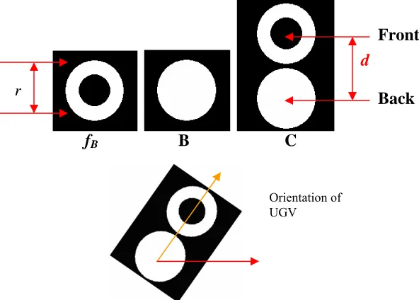
Front

Back d

r

fB B C

Orientation of UGV

Figure 5: Finding the orientation of the UGV.

The obstacles in iSpace are recognized by the template of solid circles (image B in Figure 5)

and the two concentric circles are used as template for the front of the UGV. However the single

template image (fB) is used to recognize different circles with different matching scores. (Figure 4

and Figure 5). We can apply Eq(2) to find out the maximum matching location irrespective of the

orientation of the UGV and the obstacles in the top-view space-image. The matching scores will be

in descending order as shown in Figure 4 – Highest for UGV front, medium for obstacles and

UGV back and low for any other shape existing in the workspace. Circular templates are used

(20)

once the coordinates of front and back of the UGV are obtained from template matching using

Eq(3). Where θ is the orientation angle of UGV, (xf, yf) and (xb, yb) are the co-ordinates of UGV

front and back respectively.

1

tan b f

b f

y y

x x

θ = − ⎛⎜_⎜ − ⎞ −

⎝ ⎟⎟⎠ (3)

The camera is kept at a known constant height h over the workspace; therefore it captures the

constant and predetermined area (xa x ya) of the workspace in an image of known resolution of (m

x n). The size of the template on the top of the UGV and the obstacles are also kept constant

allowing to use a template image with a fixed resolution (mtemp x ntemp). The template image fB is

(20x20) size. i.e. no zoom factor is considered. Thus the main controller does not have any

information about the size of the obstacle. Therefore, it draws a circular safety margin of radius

r

B

safe around the obstacle. Area under the safety margin is considered the part of the obstacle by the

path planning module. Details about the template matching algorithm implemented in iSpace can

be gathered from [42].

2. 3

Limitations of Template matching approach for Network based

Navigation System

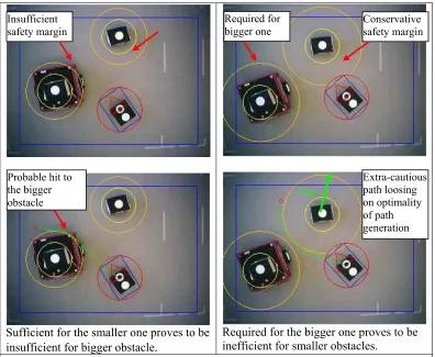
The obstacles recognized by the template matching have to be a part of a priori set of obstacles

with predefined size, shape and with predefined templates on them. Thus, the controller has no

way to extract the information about the actual size and shape of the obstacles or boundary of the

obstacles. The only information the controller has is their location (co-ordinates) in the workspace.

However, to successfully avoid an obstacle keeping the path optimality, the network controller

should have the knowledge about the actual boundaries or the radius of all the obstacles in the

(21)

might prove conservative for small obstacles loosing the efficiency on the optimal path generation

and at the same time might prove insufficient for large obstacles increasing the probability of

hitting an obstacle as evident from Figure 6. All these make the system restricted to operate in only

a few environmental patterns.

Sufficient for the smaller one proves to be insufficient for bigger obstacle.

Required for the bigger one proves to be inefficient for smaller obstacles.

Insufficient safety margin

Probable hit to the bigger obstacle

Conservative safety margin

Extra-cautious path loosing on optimality of path generation Required for

bigger one

rsafe

Figure 6: Explaining the restrictive assumptions by template matching about the size of the obstacles.

(Yellow circle around the obstacles represent the safety margin and green line from the robot to the red dot is the path drawn avoiding the obstacles considering the safety

margin.)

2. 4

Path planning using fast marching method

The input to the path generation modules is the position and orientation of the UGV (xu, yu, θu)

and obstacles’ positions from the result of the template matching module, UGV’s destination (xd,

(22)

series of points from the initial UGV position to the destination without colliding with the

obstacles. A Dijkstra-like method named the fast marching method was applied to solve the

optimal path generation problem. The fast marching algorithm is explained in brief below in

Figure 7. To find a path from A to B, let a front expand from A in all directions (a growing circle

around A in this scenario, Figure 7). Once the front touches B, we can find the shortest path by

starting at B and proceeding backwards along the path that is always perpendicular to the

expanding front as shown in Figure 7.

Figure 7: Path planning in iSpace A

B

Obstacle

UGV

20pixel

320pixel

240pixel

Platform Area

1. With Obstacles 2. Expand front around A 3. Trace back to find path

(23)

Alive

Trial

Close

Destination

Far Obstacles Far

Figure 9: Path planning using fast marching method avoiding the obstacles. Extended detail can be found in Sethian [44][45].

2. 5

Path tracking controller

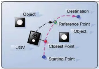
Once the optimal path is generated, the mobile robot is commanded to follow this path to the

destination. This is accomplished by approaching a sequence of reference points generated on the

desired path following a quadratic curve, as shown in Figure 8. This reference point is set at a

distance (d0) ahead from the UGV current position and closer to the destination along the path.

Appropriate speed (v, in cm/s) and turn rate (ω, in rad/s) of the mobile robot is determined once the

coefficients of this quadric curve is calculated based on the error vector (ex, ey, eθ) as described in

[37] [40]. We will again come back to this quadratic curve fitting path tracking algorithm in

Chapter III.

(24)

2. 6

Limitations of path planning method in the network based navigation

system

Thus the navigation problem is looked upon as a path tracking problem and therefore the

reference path generation is mandatory. The path tracking controller is always trying to keep the

UGV on the reference path by calculating the reference points along the path irrespective of the

UGV’s current position and distance from the reference path. If we observe, we find that the only

input path tracking controller requires is the current co-ordinates of the UGV (xc, yc,θc) and the

reference point co-ordinates (xref, yref). In each control loop iteration, the path tracking controller

has to look up the complete reference path [(x1, y1), (x2, y2), (x3, y3),…, (xn, yn)] to determine the

closest point and calculate the reference point depending upon the curvature of the path. Instead of

generating the reference path, if we are successful in calculating the reference co-ordinates for

each point in the workspace with the same or less amount of calculation than the fast marching

method, it will also automatically cut down on the real time calculation time for searching of the

reference point in the control loop.

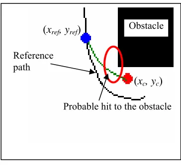
Another point of consideration is, this being a network based system, the UGV might wander

off from the path in due course of movement due to network delay. In such case, it might prove

optimal and efficient for the UGV to go the next reference position which might not lie on the

previously calculated reference path. This is explained from the Figure 9. This creates a

requirement for each point in space to have an optimal reference point toward the destination

(25)

Reference path

(xref, yref)

Probable hit to the obstacle Obstacle

(xc, yc)

Figure 11: Figure explaining the disadvantage of going for a fixed reference path

2. 7

GSM for Network delay compensation

For the network delay compensation, iSpace uses the Gain Scheduler middleware technique

introduced by Chow and Tipsuwan [41]. GSM methodology uses middleware to modify the output

of an existing controller based on a gain scheduling algorithm with respect to the current network

traffic conditions. The overall GSM operations for networked control and tele-operation can be

summarized as follows [39][40][41].

1. The feedback preprocessor waits for the feedback data from the remote system. Once the

feedback data arrives, the preprocessor processes it using the current values of network

variables and passes the preprocessed data to the controller.

2. The controller computes the control signals and sends them to the gain scheduler.

3. The gain scheduler modifies the controller output based on the current values of network

variables and sends the updated control signals to the remote system.

Thus, GSM takes care of network delay compensation satisfactorily.

Thus we can say that the delay tolerance, efficiency, accuracy, generality and optimality of

iSpace depend upon the following factors. (i) The image processing algorithm should be fast,

(26)

The output of this module should also be compatible enough with the path planning algorithm for

efficient computing time. (ii) The path planning algorithm will decide the optimality and length of

the path generated and thus probability to hit an obstacle. (iii) The time required to track that path

will also be a function of length of the path generated and the efficiency of the path tracking

algorithm. After discussing the scope of the improvement in the current iSpace, we replace the

template matching and the fast marching path planning algorithm with edge detection and

harmonic potential path planner respectively. The details of this new structure with individual

modules as the part of an efficient integrated navigation systems against the previous systems are

(27)

CHAPTER III

– New Structure of iSpace

After discussing the current setup of iSpace as a network based integrated navigation system,

and the scope of improvement, this chapter explains the new structure and the component details

for iSpace. We use edge detection instead of template matching and harmonic potential field

functions for path planning replacing the fast marching method.

3. 1

Edge detection to extract the contents of the iSpace environment

Edge detection is a classic early vision tool to extract discontinuities from the image as features.

Thus all the discontinuities which are more or less obstacle boundaries will be represented by

binary edges in the edge detected image of the UGV workspace [30][29]. We call the edge

detected image of the workspace as an “Edge map”. Before explaining the mathematical and

functional properties of the edge detection, Figure 8 explains the effect of taking the first and

second derivative of a 1-D function. We can observe that the magnitude of the first derivative

(magnitude of the gradient) can be used for detecting the presence of the edge in an image and the

sign of the second derivative can be used to determine whether an edge pixel lies on the dark or

light side of the edge, in brief it can be used to find out the direction of the gradient. Thus zero

(28)

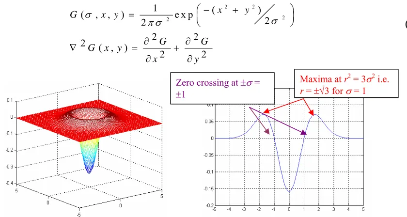
Therefore, the edge detector we use has two branches. One branch processes the workspace

image I with a circularly symmetric approximated Laplacian of 2-D Gaussian (LoG) operator to

find out the second derivative of the image which will be used to find out the zero crossings in the

image as the potential edges.

2 2

1 ₍ ₎

( , , ) e x p

2 2

2 _{( , )}

2 2

x y

G x y

G G

G x y

x y

σ _σ

π σ

⎛ − + ⎞

= _⎜ _⎟

⎝ ⎠

∂ ∂

∇ = +

∂ ∂

Profile of a horizontal line (For e.g. Cross section of an image) First derivative gives high magnitude at the edges. Threshoding will leave out the edges. Second derivative gives the directional gradient of the edges and their potential locations

Figure 12 : Explaining the significance of the first and second derivative (This is for a 1-D cross section of an image)

(4)

Maxima at r2 = 3σ2 i.e.

r= ±√3 for σ = 1

Zero crossing at ±σ =

±1

Figure 14: ∇2G(σ,r)versus r with σ = 1

Figure 13: 3-D plot of 2 ( , , )at σ = 1 y

(29)

Let r2 = x2 + y2 Thus Laplacian of G(σ, r) with respect to r is given in Eq(5).

(

)

(

)

2 exp 2 1 2 2 4 2 2 2 2 σ σ σ

πσ r r

G ⎟ −

⎠ ⎞ ⎜ ⎝ ⎛ − =

∇ (5)

The Figure 12shows the cross-section of the circularly symmetric function representing

as expressed in Eq(5). From Eq(5), we have, = 0 at r

) , , ( 2 y x Gσ ∇ ) , ( 2 r Gσ

∇ _∇2_G(_σ,_r) 2 = σ2. We also observe

that from Figure 12 thatthe zero crossing is at r = ±σ

i.e. x2+y2=σ2 (6)

Eq(6) is the equation of the circle in the plane z = 0 (radius σ and center at (0, 0)) passing through

all the zero-crossing point. To form the approximate 7 x 7 kernel representing the circularly

symmetric LoG, we sample at (x, y) = (-3, -3) to (3, 3). To find out the value of r at which

the LoG attains its maxima, we equate the third derivative ∇

) , (

2_G_σ _r

∇

3_G(_σ_{,r) to zero .}

(

)

3 0 2 exp 2 2 1 0 ) , ( 2 2 2 2 2 2 2 2 6 3 σ σ σ σ σ πσ σ = ∴ = − ⎟⎟ ⎠ ⎞ ⎜⎜ ⎝ ⎛ + − ∴ = ∇ r r r r G

Thus, maxima is attained at r2 = 3σ2 (Figure 12). Therefore, to have maxima at r = 2 i.e. second neighboring pixel from the center pixel, r = 2 ∴σ = ±2/√3. We sample the circularly symmetric

LoG and get the following discrete approximation as 7 x 7 kernel.

(30)

However, we know that elements of the kernel should sum up to zero because they are the

discrete representation of Laplacian of Gaussian Eq(5) whose average value is zero. (Proof below -

Integration from – ∞ to +∞ is zero).

(

)

(

)

( ) (

)

0 2 exp 2 1 2 exp 2 1 2 2 2 2 2 2 2 4 2 2 2 2 = ⎥⎦ ⎤ ⎢⎣ ⎡ − ₋ = − ⎟ ⎠ ⎞ ⎜ ⎝ ⎛ − = ∇ ∞ ∞ − ∞ −∞ = ∞ −∞ =

∫

σ σ πσ σ σ σ πσ r r dr r r dr G r r

And if the sum of elements is not zero, after convolving the kernel with the image (I), the

brightness factor will not be maintained, it will however be shifted with a factor of the sum of the

elements. This is more important for iterative algorithms and can be ok for convolving once as we

do in case of this edge detection. But for a good practice, we adjust the elements by subtracting the

sum from each element such that their sum is zero.

LoG =

0.0363 0.1181 0.2438 0.3032 0.2438 0.1181 0.0363 0.1181 0.3687 0.4927 0.4117 0.4927 0.3687 0.1181 0.2438 0.4927 -0.4107 -1.5261 -0.4107 0.4927 0.2438 0.3032 0.4117 -1.5261 -3.5688 -1.5261 0.4117 0.3032 0.2438 0.4927 -0.4107 -1.5261 -0.4107 0.4927 0.2438 0.1181 0.3687 0.4927 0.4117 0.4927 0.3687 0.1181 0.0363 0.1181 0.2438 0.3032 0.2438 0.1181 0.0363

⎡ ⎤ ⎢ ⎥ ⎢ ⎥ ⎢ ⎥ ⎢ ⎥ ⎢ ⎥ ⎢ ⎥ ⎢ ⎥ ⎢ ⎥ ⎢ ⎥ ⎣ ⎦ LoG

I = ⊗I LoG

The zero crossing contours from this operator are taken as the candidate edges. Such a map is

extremely noisy and practically useless as shown in Figure 13 unless the contours corresponding to

(31)

Figure 15: workspace image I and its zero crossing contour for I⊗ ∇2G

The filtering adopted here is based on the strength of the edge, i.e. its contrast. Therefore, the

second branch for the edge detection block is an approximated first derivative gradient operator of

2-D Gaussian function with x-direction and y-direction mean (μx and μy) as zero (Eq 4). It is used

to produce an estimate of the contrasts. The 2-D Gaussian function is shown in (4) where σ is the standard deviation deciding the spread of the bell curve shown in Figure 14.

.

2 2

( , )

1 ( )

( , , ) exp

2 2

T

G G

G x y

x y

G σ x y _σ

πσ

⎡∂ ∂ ⎤

∇ _{= ⎢} _⎥

∂ ∂

⎣ ⎦

⎛− + ⎞

= _⎜ _⎟

⎝ ⎠

(7)

(8)

(32)

Image

I

Laplacian of

Gaussian ∇

2

_G

Gradient of

Gaussian ∇G

Zero Crossing

Magnitude

Threshold

(C)

Edge

Map

E

Figure 17: Complete edge detector block diagram

Applying the first derivative Gaussian to the image is equivalent to first blurring the image

with a kernel bigger in the middle and then differentiating to get the gradient as shown in

Eq(9)[28]. If the contrast of an edge is above a certain threshold, the edge is accepted as authentic;

otherwise it is rejected as noise. This is introducing low-pass filtering which should to some extent

suppress the effect of wideband noise from the edge map removing the false edges.

( ) G

d I G I

x x ∂ ∂ = ⊗ = ⊗ ∂ ∂ ⎟ ⎠ ⎞ ⎜ ⎝ ⎛− + − = ∂ ∂ 2 2 2 4 ₂ ) ( exp 2 / ) , , ( _σ πσ

σ x x y

x y x G 2 ) ( exp 2 / ) , , ( 2 2 2

4 ⎟_⎠

⎞ ⎜ ⎝ ⎛− + − = ∂ ∂ _σ πσ

σ _x _y _y y x y

G

(9)

(10)

Figure 19: Graph representing ∂G(σ,x,y)/∂y Figure 18: Graph representing∂G(

σ

,x,y)/∂x

(33)

I(x, y) is the original grey-scale image from the network camera. The first derivative with

respect to x, IGx(x, y) and with respect to y, IGy(x, y) of I(x, y) is thus obtained by using Eq(11) and

Eq (12).

( , , )

( , ) ( , )

Gx

G x y

I x y I x y

x σ ∂

= ⊗

∂ (11)

Gy( , ) ( , ) ( , , )

G x y

I x y I x y

y σ ∂

= ⊗

∂ (12)

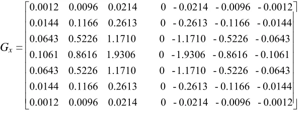
To form the 7x7 approximated kernels representing ∂G(

σ

,x,y)/∂x and

∂

G

(

σ

,

x

,

y

)

/

∂

y

, let us sample the 2-D curves shown in (Figure 16andFigure 17) at x = -3, -2, -1, 0, 1, 2, 3 and y = -3, -2,

-1, 0, 1, 2, 3 forming a sampling distance Δs = 1 as shown in Table 1. Here sampling values of x

and y represent the position of the pixel relative to the center pixel with x = 0 and y = 0 at which

the kernel is applied to find the gradient at that point.

Table 1: Sampling ticks with Δs = 1 to form 7x7 approximated kernel for ∂G(σ,x,y)/∂x and y

y x

G ∂

∂ (σ, , )/ at σ= 1

(-3, -3) (-2, -3) (-1, -3) (0, -3) (1, -3) (2, -3) (3, -3)

(-3, -2) (-2, -2) (-1, -2) (0, -2) (1, -2) (2, -2) (3, -2)

(-3, -1) (-2, -1) (-1, -1) (0, -1) (1, -1) (2, -1) (3, -1)

(-3, 0) (-2, 0) (-1, 0) (0, 0) (1, 0) (2, 0) (3, 0)

… … …

… … … (3, 3)

As mentioned before σ will decide the spread of the bell curve over the 7x7 = 49 pixels. Let us

(34)

forth row of the kernel. The immediate neighbors of the center pixel (0, 0) in the x-direction i.e. at

(-1, 0) and (1, 0), should have the maximum weight in the kernel considering the intuitive

assumption that immediate neighboring pixels have more contribution in deciding the edge

presence at any pixel and therefore sampled value of ∂G(σ,x,y)/∂x should be maximum at x = 1

and -1. We find out the value of σ where the value of first derivative ∂G(σ,x,y)/∂xattains its

maximum at (-1, 0) and (1, 0) by equating the second derivative 2 ₍ _,₁_,₀₎_/ 2 to zero. x G ∂ ∂ σ

( )

1 at 0 / ) 0 , 1 , ( 2 1 exp 2 1 2 1 / ) 0 , 1 , ( 2 ) ( exp 2 1 2 / ) , , ( 2 2 2 4 6 2 2 2 2 2 2 4 6 2 2 2 = = ∂ ∂ ∴ − ⎟⎟ ⎠ ⎞ ⎜⎜ ⎝ ⎛ − = ∂ ∂ ⎟ ⎠ ⎞ ⎜ ⎝ ⎛− + ⎟⎟ ⎠ ⎞ ⎜⎜ ⎝ ⎛ − = ∂ ∂ σ σ σ πσ πσ σ σ πσ πσ σ x G x G y x x x y x G

Therefore we have the maxima of the absolute value of the first gradient of the Gaussian in the

x-direction at σ = 1, as confirmed by the Figure 18

Figure 20: Cross-section of the ∂G(σ,x,y)/∂xat a

plane y = 0 withσ = 1

Figure 21: A 20x scaled 7 point approximation of

x x

G ∂

∂ (1, ,0)/

The 7 x 7 kernel Gx approximating the first derivative of 2-D Gaussian with respect to x at σ = 1 is

(35)

Gx = ⎥ ⎥ ⎥ ⎥ ⎥ ⎥ ⎥ ⎥ ⎥ ⎦ ⎤ ⎢ ⎢ ⎢ ⎢ ⎢ ⎢ ⎢ ⎢ ⎢ ⎣ ⎡ 0.0012 0.0096 0.0214 0 0.0214 0.0096 0.0012 0.0144 0.1166 0.2613 0 0.2613 0.1166 0.0144 0.0643 0.5226 1.1710 0 1.1710 0.5226 0.0643 0.1061 0.8616 1.9306 0 1.9306 0.8616 0.1061 0.0643 0.5226 1.1710 0 1.1710 0.5226 0.0643 0.0144 0.1166 0.2613 0 0.2613 0.1166 0.0144 0.0012 0.0096 0.0214 0 0.0214 0.0096 0.0012

Similarly, the gradient in y-direction Gy approximating

∂

G

(

1 ,

x

,

y

)

/

∂

y

can be directly written as

transpose of the Gx

Gy =

⎥ ⎥ ⎥ ⎥ ⎥ ⎥ ⎥ ⎥ ⎥ ⎦ ⎤ ⎢ ⎢ ⎢ ⎢ ⎢ ⎢ ⎢ ⎢ ⎢ ⎣ ⎡ 0.0012 0.0144 0.0643 0.1061 0.0643 0.0144 0.0012 -0.0096 0.1166 0.5226 0.8616 0.5226 0.1166 0.0096 -0.0214 0.2613 1.1710 1.9306 1.1710 0.2613 0.0214 -0 0 0 0 0 0 0 0.0214 0.2613 1.1710 1.9306 1.1710 0.2613 0.0214 0.0096 0.1166 0.5226 0.8616 0.5226 0.1166 0.0096 0.0012 0.0144 0.0643 0.1061 0.0643 0.0144 0.0012

Figure 22: ∂G(1,x,y)/∂x Figure 23: A 20x scaled 49(7x7) point approximation of ∂G(1,x,y)/∂x

3. 2

Results of edge detection

Figure 22 shows a few sample images from the actual iSpace setup in ADAC lab with different

environment such as textured background in Example 5 and Example 6, cluttered with many

obstacles in Example 2 and Example 6 and their corresponding Edge maps. The edge maps can be

(36)

E(xi, yj) = 1 if (xi, yj) ∈ΩB B

= 0 if (xi, yj) ∉ΩB for all (i, j)

Where E(x, y) is the image representing the edge map and ΩB is the set of edge points

including the boundary points for all obstacles in workspace.

Figure 24: Top view images I(x, y) with their corresponding edge maps E(x, y).

Approximation of the 2-D waveforms to form kernel is learnt from Snyder, Qi [28]

3. 3

2-D HPF planner for path planning

The Harmonic function on a domain Ω ⊂ ℜ2_{is a function which satisfies the following}

Laplace equation – Eq(14).

(13)

(14)

Example 1 Example 2 Example 3

Example 4 Example 5 Example 6

0 2 2 2 2

2 ₌ ₊ ₌

y x h

δ φ δ δ

φ δ φ

The use of potential field in motion planning was introduced by Khatib [2]. The obstacles were

represented by the repelling force and the point of destination was represented by the attractive

force. Unfortunately, the setting Khatib suggested suffered from a deadlock problem known as the

local minima problem. Laplace as a harmonic function was proposed by Connolly et al. [3][5] to

(37)

local minima may be intuitively demonstrated by considering the two-dimensional version of

Laplace’s Equation. Consider the two curves which are the x and y cross-sections of φ at some

point p0. If the second derivatives of φ are individually not zero at p0, then two curves in question

must have second derivatives of opposite sign forφ to satisfy Eq(14) . Assuming that φ∈C2, this

implies that one curve must be concave upward and the other must be concave downward. Thus

we have that either φ is planar at p0, or that there is a direction outward from p0 in which φ

decreases, and another in which φ increases. Therefore, in any open region where Laplace’s

equation holds, local extrema of φ cannot exist. More formally, if a function φ satisfies Laplace’s

equation on some region Ω ⊂ ℜn_{, then any critical points of the function in the interior of that}

region must be saddle points, since local extrema of the function are not possible there. If the

effector reaches a saddle point, and it is not near the goal, then there must be a way out. This exit

from this critical point may be found by performing a search in the neighborhood of the critical

point. In this context the path from the source to the destination consists of these saddle points.

Here, we use HPF in Dirichlet’s settings. With these settings, obstacles are raised to a constant

high potential and while goal regions are kept at low potential as explained in Eq(15). The

resulting potential is then constrained by ∇2_φ_{= 0. With this manner the gradient of}_φ_{is aligned}

with the surface normal of the obstacles and thus driving the UGV away from obstacles.

2

T T

( , ) 0 , Ω

subject to

( , ) 1 , Γ

and ( , ) 0 ( , ) ( , )

∇ ≡ ∈

= ∈

= =

x y x y

x y x y x

φ φ

φ

(15)

(38)

where_∇2is the Laplace operator, Ω is the workspace of the UGV (Ω ⊂ ℜ2), Γ is the boundary

of the obstacles, and(xT,yT)is the target point. The obstacle free path to the target is generated by

traversing the negative gradient of( )φ i.e. (−∇φ).

Numerical solutions for the Laplace’s equation are readily obtained from the Finite Difference

Method. Let φ (x, y) be a function which satisfies Laplace equation and let u(xi, yi) represents

discrete regular sampling of the φ on a grid. A central difference formula for the second

derivatives of φ can be derived using Taylor’s series. Higher order terms are neglected. [3]

2

1 1

2

1 1

2

( , ) 2 ( , ) ( , ) ( , )

( , )

12

( , ) 2 ( , ) ( , ) ( , )

( , )

12

i j i j i j xxxx i j

xx i j

i j i j i j yyyy i j

yy i j

u x y u x y u x y h u y

x y

h

u x y u x y u x y k u x

x y

k

ξ φ

η φ

+ −

− +

= −

− +

= −

The fourth order terms can be neglected being very small. h and k are the step size in x and y

direction respectively. Assuming h = k = 1, we can write

2

1 1 1 1

( ,_i _j) ( _i , _j) ( _i , _j) ( ,_i _j ) ( ,_i _j ) 4 ( ,_i _j)

h φ x y =u x ₊ y +u x ₋ y +u x y ₊ +u x y ₋ − u x y

For φ(x, y) to satisfy the Laplace equationh2φ( ,x_i y_j) 0= , we

1 1 1 1

( , ) ( , ) ( , ) ( ,

( , )

4

i j i j i j i j

i j

u x y u x y u x y u x y

u x y = + + − + + + − ) (16)

Thus with Laplace equation, this method simply consists of repeatedly replacing each grid points

with the average of its neighbors using successive relaxation. Terminate when the array u contains

a sampling φof where every non-boundary condition node has a neighbor with a smaller value

(39)

3. 4

HPF and Edge detection Merged together

The close relation between Edge detection and HPF is what makes this path planning algorithm

so interestingly efficient and flexible. As with Edge detection the obstacle boundaries are already

raised to a high potential (binary edges, φ = 1) and all the other points in the workspace which are

not on the obstacle contour are at the low equal potential conditions (UGV movement area φ = 0), as we look at the Eq(13) and Eq(15). ΩB nothing but boundaries of the obstacle, Γ, raised to a high

potential. Thus it provides the exact raw data required for HPF in Dirichlet’s setting to create the

gradient direction matrix. It was also proven that the potential function in any connected

component without goals will converge to a constant potential in that UGV configuration space [3].

All the connected components in the edge map represent the obstacle boundary, so with this

principle, the obstacles in the workspace will be represented by a high potential repelling the UGV

away from it., The destination point is then represented by the lowest potential (φ = -1). The

normalized gradient at each point will then represent the directional guidance at each point in the

workspace matrix avoiding the obstacles represented by the edge map towards the destination

point. Vx and Vy are the 2-D arrays of negative directional gradient of the workspace in x and y

direction respectively. 2 2 ⎟ ⎠ ⎞ ⎜ ⎝ ⎛ ∂ ∂ + ⎟ ⎠ ⎞ ⎜ ⎝ ⎛ ∂ ∂ ∂ ∂ − = y x x V_x φ φ φ And 2 2 ⎟ ⎠ ⎞ ⎜ ⎝ ⎛ ∂ ∂ + ⎟ ⎠ ⎞ ⎜ ⎝ ⎛ ∂ ∂ ∂ ∂ − = y x y Vy φ φ φ (17) Where 2 ) , 1 ( ) , 1

(x y x y

x − − + = ∂

∂φ φ φ _and

2 ) 1 , ( ) 1 , ( + − − = ∂

∂ x y x y

y

φ φ

φ

Thus HPF planner will be used as directional guidance for the UGV. However, the velocity

(40)

Figure 23 shows the result of the HPF planner after applying them on the edge map. Here the

edge maps are created synthetically to test the algorithm. However, the Figure 24 shows the HPF

results with actual iSpace workspace image edge maps. The arrows represent the gradient direction

at each point in the planner. We observe that the HPF plan of the workspace is the function of

obstacle boundaries and the destination point. Thus HPF converts the edge map into a “Region to

Point Guidance Function”.

(41)

Goal point chosen, shown as the smallred

dot

Goal point chosen, shown as the small

red dot

Figure 26: Figures showing the result of HPF planner – Region to Point guidance function.

3. 5

HPF, a region to point guidance function, combined with the network

based controller

The important feature of HPF planner to convert the edge map into a region to point guidance

function makes it easily compatible with the quadratic curve fitting UGV movement controller

reaching to the goal more efficiently. The basic principle of this control algorithm as explained in

[29] by Yoshizawa et al. is that a reference point is moved along a desired path so that the length

between the reference point and the UGV is kept in some distance. Control (velocity) commands

are generated for the UGV to reach that reference position from the current position. (Figure 8,

(42)

the gradient array of HPF has features which enable to use this method more efficiently without

advanced knowledge of the path being tracked. Once the complete 2-D gradient matrix is

calculated, all the directional information required for the UGV to reach the goal from any point in

the workspace is available in the HPF planner as shown in Figure 24. In other words, every point

in the region will have a guidance vector associated with it directing it towards next reference

position leading towards the goal. This can be treated as the same reference position required by

the quadratic curve controller as explained. Thus, the important Region to point guidance property

of HPF makes it a more efficient path planner to be combined with quadratic controller without the

reference path generation. As shown in Figure 24, the image to the right is the HPF gradient of the

left image with destination as shown. All the points in the workspace steer the UGV to the goal

showing that the gradient directions are the function of the goal point, not the source point. So thus

the problem is converted to a “goal seeking” problem from a “path tracking” problem. And the

“path generation” module is replaced by “HPF planner” module. We need to compute the gradient

array (V). The reference position ( ,x_R y_R) for each current position ( , )x y is calculated from the

gradient array of the HPF (∇φ). Vx and Vy are the 2-D arrays of x- and y-components of ∇φ

respectively as described in Eq(17). Then each reference position R x( ,₀ y₀)= ( ,x_R y_R) is calculated

as shown in Eq(18).

) , (

0 0 0

y x V y y

y x V x x

y R

x R

+ =

(18)

We can choose the reference position at a look-ahead distance (d0) from the current position.

Let the discrete look-ahead distance be represented byδL . IfδL=2 , then for the current

position

(

x0,y0

)

, R x( ,0 y0)=( ,x2 y2), as explained in Figure 25. Thus for (δL >1) , Eq(18) is

(43)

Figure 27: HPF gradient image enlarged explaining the concept of discrete look-ahead distance.

The accuracy of the path traced will be sensitive to the look-ahead distance (d0) selected as the

quadratic curve controller will d0 curve fitting (y = Ax2) between the current ( ,x0 y0) and the reference point( ,xR yR). The magnitude of the speed v and the turn-rate ω is proportional to the

distance d0 between( ,x y0 0)and( ,xR yR). Small δL will keep the UGV trajectory close by the desired path. However the time to complete the path will increase because of the small v and ω (as shown

in Figure 27). If δL is large, (e.g. δL= 6) then d0 will be large. The quadratic curve controller will

approximate the path between( ,x y₀ ₀)and( ,x₆ y₆), which may not match the exact path generated by

the HPF planner going through

{

( ,x₀ y₀), ( , ),..., ( ,x y₁ ₁ x₆ y₆)

}

. Thus, distance error from the ideal path

will increase increasing the probability of hitting nearby obstacles in case of large network delays

as shown in the third image in Figure 26.

δL = 1, Network delay = 0.1mS

T = 27 seconds

δL = 8, Network delay = 0.1mS T = 16 seconds

δL = 8, Network delay = 0.6mS

(44)

0.05 0.1 0.15 0.2 0.25 0.3 0.35 0.4 0 0.02 0.04 0.06 0.08 0.1 0.12

Look-ahead distance in meters

Di st an ce e rr o r o n met er

s Max Delay_{Mean delay}

Median Delay

0 0.05 0.1 0.15 0.2 0.25 0.3 14 16 18 20 22 24 26 28

Look ahead dist in meters

Tot al t im e t o r ea c h t he go al i n s eco nds

Figure 29: Distance error increases and total time to reach the goal decreases with increase in δL.

As described in [37] and [41], the quadratic path tracking controller fits the curve y = An x2

once the current position (xc, yc, θc) and the reference position (xref, yref) are known. We know that

the distance d0 at which the reference point is to be located from the current position is calculated

by the quadratic path tracking controller at each control loop, depending upon the curvature of the

path (An) at that current position by Eq(19a) [37]. Thus the discrete δL should be proportional to

d0. Thus we calculate δLusing Eq(19b). And then v and ω are calculated using Eq(19c). To choose

the reference point to start with, we take δLas its minimum value i.e. δL= 1. Thus (e_x, e_y, eθ) the

error vector is calculated for (xc, yc, θc) and (xref, yref) .

max 0 2 0 ( ) 1 y x x D e d

An sign e d

e A d L G

β

δ

= = + ⎢ ⎥ = ⎢ ⎥ ⎣ ⎦ (19a) n (19b)

( ) 2

1 | |

n x n n

K sign e v K An K

An

α _ω

= =

+ = ⋅ ⋅ (19c)

GD is a constant representing the actual physical distance in meters corresponding to i.e the

workspace distance between the two pixels of the workspace image (I) distance representing the

(45)

distance. GD is calculated as Eq(20) with workspace image resolution (m x n) and the area covered

by the network camera i.e. workspace size (xa x ya). For iSpace, image resolution is 320 x 240 and

workspace size is (4m x 3m) ∴ GD = 0.0125 m

0.0125

a a

D

x y

G m

m n

= = =

Thus at a high curvature point, d0 will be small, giving rise to a small δL (look-ahead distance).

The UGV will run slowly being more cautious on the turn. On the other hand if the path is a

straight line (low curvature point), then the reference point will be chosen at comparatively a larger

distance from current position making the UGV move faster. Thus dynamically choosing the

look-ahead distance will incorporate optimality between the path tracking accuracy and the time

required to reach the goal. Thus the HPF planner successfully provides the features required by the

quadratic curve fitting controller to calculate the v and ω for differential drive UGV.

(20)

(46)

CHAPTER IV

– Comparison of the new

modules with the previous modules

In this chapter, we formally compare not only each previous module with the new module but

also emphasize on the performance improvement in iSpace as a whole network based integrated

navigation system because of the compatibility achieved between the modules by introducing edge

detection and HPF planner.

4. 1

Comparison of edge detection with template matching for iSpace

(1) Restrictions on the contents of the environment – As we mentioned earlier, that template

matching imposes the restrictions on the contents in the iSpace environment to be a part of a

priori set with specified templates. Requirement of templates on obstacles is not a reasonable

idea. This restriction is removed with implementation of edge detection. With edge detection,

any real world obstacle can be expected to be detected without template. Figure 22 shows that

edge detection works for many different varieties of obstacles and environment cases in iSpace

and this is definitely a quality addition towards improving the generality of iSpace.

(2) Definite knowledge of obstaclesboundaries – Comparing to template matching where the

main controller only knows the location of the center of the template on the obstacle without

having any quantitative and definite knowledge about the size and shape of the obstacle, edge

detection marks the boundaries distinctively. Thus the path planning algorithm has better

knowledge about the contents of 2-D space of interest for optimal path planning. Both the

(47)

Figure 30: Template matching and Edge detection outputs for the same workspace image

(3) Computational complexity – Let us consider both the template matching and the edge

detection algorithms to learn the improvement in the computational efficiency with edge

detection. Here, we consider the major parts of the calculations involved in both the algorithms.

Table 2: Calculations for Template matching computations Template matching

Steps Number of Computations

Thresholding the grey scale image I(x, y) to get

black and white image.

(m x n) comparisons

m = 320 and n = 240

76800

Matching operations as per

(

)

2

( , ) ( , )

( i j , ) 1 i j

A B A B

j i

h f f f f

⎛ ⎜

= _⎜ − − _⎟

⎜ ⎟

⎝

∑ ∑

⎞⎟ ⎠

for the

image I(m x n) with the template image fB

(mtemp x ntemp)

((m- mtemp) x (n- ntemp)) x (mtempx ntemp)

m = 320, n = 240, mtemp = 20 and ntemp = 20

26400000

(48)

(Tthreshold) which is the signature value for the

template presence.

if ( ( , )i j , ₎

A B

h f f > T_threshold then template present at

(i, j) else template absent.

m = 320 and n = 240

76800

Filter out the other matching scores which are

above the Tthreshold but lie on the immediate

neighborhood of the center position of the

template.

This depends upon the number of score

matching say Nn and number of obstacles are

No then

number of operations are < Nn x No

Sorting the thresholded values to distinguish

between the front and back of the UGV from

the obstacles.

This depends upon the number of score

matching i.e. number of obstacles present –

assume ksort

Approximated total (CTemplateMatching) (26553600 + ksort)

Table 3: Calculations for Edge detection computations Edge detection

Steps Number of Computations

(320 240) (7 7)

I × ⊗Gx × (m-7 _x n-7) _x (7 _x 7) = 3573521

(320 240) (7 7)

I × ⊗Gy × (m-7 _x n-7) _x (7 _x 7) = 3573521

Let M = (I⊗Gx)2+ ⊗(I Gy)2

I(x, y) = 0 if M(x, y) <= C

= 1 if M(x, y) > C, for all the pixels in I(x, y)

(m x n) + (m x n) =

153600

(320 240) (7 7)

An Edge-detection and HPF Based Intelligent Space - A Network Based Integrated Navigation System.

ABSTRACT

A

E

-

HPF

I

S

–

A

N

B

I

N

S

BIOGRAPHY

ACKNOWLEDGEMENTS

TABLE OF CONTENTS

LIST OF TABLES

LIST OF FIGURES

σ

CHAPTER I

– Introduction

CHAPTER II

– Introduction to iSpace as a

Network based Integrated Navigation system

2. 1

Different components in iSpace

(

)

2. 2

Template matching for content recognition

(

)

∑ ∑

2. 3

Limitations of Template matching approach for Network based

Navigation System

2. 4

Path planning using fast marching method

2. 5

Path tracking controller

2. 6

Limitations of path planning method in the network based navigation

system

2. 7

GSM for Network delay compensation

CHAPTER III

– New Structure of iSpace

3. 1

Edge detection to extract the contents of the iSpace environment

(

)

(

)

(

)

(

)

(

)

( ) (

)

∫

∫

Image

I

Laplacian of

Gaussian ∇

G

Gradient of

Gaussian ∇G

Zero Crossing

Magnitude

Threshold

(C)

Edge

Map

E

σ

_G