ABSTRACT
QIAN, TAO. End-to-end Predictability for Distributed Real-Time Systems. (Under the direction of Rainer Frank Mueller.)
Distributed real-time systems impose a number of requirements, such as scalability, reliabil-ity, predictabilreliabil-ity, and high computational throughput. These demands can be met by designing protocols for participating nodes and network infrastructures specifically for these requirements. Unlike other distributed systems whose main objective is to provide high throughput or low request latency, our system addresses one additional significant requirement raised by real-time systems, namely end-to-end response time predictability for distributed real-time systems. Thus, the goal of our system is to execute distributed real-time tasks within their deadlines imposed by the clients. One of the potential applications is a wide-area monitoring system (WAMS) for power grid state monitoring and control. In such a system, state monitoring devices periodi-cally gather data from the power grid infrastructure scattered over a wide area and the WAMS subsequently requests these data in a timely fashion.
The followings are the key contributions of this work:
1. To support storing and fetching wide-area monitoring data in a timely fashion, we imple-ment a real-time storage system based on the Chord protocol. We employ an application-level task scheduler to arbitrate the execution of the distributed tasks for wide-area moni-toring. In addition, we formally define the pattern of the workload and use queueing theory to stochastically derive the time bound for response times of these data requests. On the basis of the queueing model, the system can provide probabilistic deadline guarantees for data requests.
2. To realize the deadlines of data requests and schedule urgent requests first, we implement an earliest deadline first (EDF) based packet scheduler to transmit data requests via the underlying network infrastructures. This packet scheduler runs on end nodes. In addi-tion, we utilize the hierarchical token bucket (HTB) traffic control mechanism provided by Linux to implement a bandwidth sharing policy. This policy regulates the message traffic that is transmitted via the network. The hybrid scheduler decreases the variance of network transmission delays, which increases the predictability of end-to-end delays for distributed real-time tasks.
communicating tasks must be managed actively. We implement a static routing algorithm to derive the forwarding paths for real-time packets according to the network capability (i.e., buffer size and computation speed of network devices). In addition, we implement a real-time packet scheduler, which runs on network devices to enforce the packet scheduling policy derived by the routing algorithm under stable network conditions.
c
Copyright 2017 by Tao Qian
End-to-end Predictability for Distributed Real-Time Systems
by Tao Qian
A dissertation submitted to the Graduate Faculty of North Carolina State University
in partial fulfillment of the requirements for the Degree of
Doctor of Philosophy
Computer Science
Raleigh, North Carolina
2017
APPROVED BY:
Aranya Chakrabortty Matthias Stallmann
Guoliang Jin Rainer Frank Mueller
BIOGRAPHY
ACKNOWLEDGEMENTS
TABLE OF CONTENTS
List of Tables . . . vi
List of Figures . . . vii
Chapter 1 Introduction . . . 1
1.1 Real-Time Systems . . . 1
1.2 Distributed Real-Time Systems . . . 2
1.3 Temporal Requirements . . . 4
1.4 Contributions . . . 5
1.5 Hypothesis . . . 6
1.6 Organization . . . 7
Chapter 2 A Real-time Distributed Hash Table . . . 8
2.1 Introduction . . . 8
2.2 Design and Implementation . . . 10
2.2.1 Chord . . . 10
2.2.2 The pattern of requests and jobs . . . 12
2.2.3 Job scheduling . . . 14
2.2.4 Real-time DHT . . . 16
2.3 Analysis . . . 16
2.3.1 Job response time on a single node . . . 16
2.3.2 End-to-end response time analysis . . . 21
2.3.3 Quality of service . . . 21
2.4 Evaluation . . . 24
2.4.1 Low workload . . . 24
2.4.2 High workload . . . 27
2.4.3 Prioritized queue extension . . . 28
2.5 Related work . . . 30
2.6 Conclusion . . . 31
Chapter 3 Hybrid EDF Packet Scheduling for Real-Time Distributed Systems 33 3.1 Introduction . . . 33
3.2 Design . . . 36
3.2.1 Partial-EDF Job Scheduler . . . 36
3.2.2 Time-difference Table . . . 41
3.2.3 EDF Packet Scheduler and Bandwidth Sharing . . . 42
3.3 Real-Time Distributed Storage System . . . 44
3.3.1 DHT . . . 44
3.3.2 Hybrid EDF Scheduler Integration . . . 45
3.4 Experimental Results and Analysis . . . 47
3.4.1 Bandwidth Sharing Results . . . 48
3.4.2 EDF Packet Scheduler Results . . . 50
3.5 Related work . . . 53
3.6 Conclusion . . . 54
Chapter 4 A Linux Real-Time Packet Scheduler for Reliable Static Routing . 55 4.1 Introduction . . . 55
4.2 Design . . . 57
4.2.1 System Model and Objectives . . . 57
4.2.2 Message Scheduler . . . 60
4.2.3 Routing Algorithm . . . 63
4.2.4 Forwarding Path Candidate . . . 65
4.3 Implementation . . . 65
4.3.1 Message Structure and Construction . . . 66
4.3.2 Forwarding Table Structure . . . 67
4.3.3 Virtual Switch Implementation . . . 68
4.4 Evaluation . . . 69
4.4.1 Single Virtual SDN Switch Result . . . 70
4.4.2 Multiple Virtual Switches Result . . . 73
4.4.3 Routing Algorithm Demonstration . . . 74
4.5 Related Work . . . 76
4.6 Conclusion . . . 78
Chapter 5 Conclusion and Future Work . . . 80
5.1 Conclusion . . . 80
5.2 Future Work . . . 82
LIST OF TABLES
Table 2.1 Finger table forN4 . . . 12
Table 2.2 Finger table forN20 . . . 12
Table 2.3 Types of Messages passed among nodes . . . 14
Table 2.4 Notation . . . 19
Table 3.1 Finger table forN4 . . . 45
Table 4.1 Notation . . . 58
Table 4.2 Forwarding Table . . . 68
Table 4.3 Message Scheduler Variables . . . 68
Table 4.4 Test Workload in Single Switch Experiment . . . 71
Table 4.5 Expected Response Time vs Message Drop Rate . . . 73
Table 4.6 Real-time Message Flows in Demonstration . . . 75
Table 4.7 Forwarding Path Candidates . . . 76
LIST OF FIGURES
Figure 1.1 Wide-Area Monitoring System . . . 3
Figure 1.2 Distributed Systems Abstract . . . 4
Figure 2.1 PDC and Chord Ring Mapping Example . . . 11
Figure 2.2 Low-workload Single-node Response Times (4 nodes) . . . 25
Figure 2.3 Low-workload Single-node Response Times Distribution (4 nodes) . . . . 26
Figure 2.4 Low-workload End-to-end Response Times Distribution . . . 27
Figure 2.5 High-workload Single-node Response Times (8 nodes) . . . 28
Figure 2.6 High-workload Single-node Response Times Distribution (8 nodes) . . . . 29
Figure 2.7 High-workload End-to-end Response Times Distribution . . . 30
Figure 2.8 End-to-end Response Times Distribution Comparison . . . 31
Figure 3.1 Partial-EDF Job Scheduler Example (1) . . . 37
Figure 3.2 Partial-EDF Job Scheduler Example (2) . . . 38
Figure 3.3 Chord Ring Example . . . 45
Figure 3.4 Network Delay Comparison (1) for Delay Clusters (ms) . . . 49
Figure 3.5 Network Delay Comparison (2) . . . 50
Figure 3.6 Deadline Miss Rate Comparison . . . 51
Figure 4.1 Message Phases on Node . . . 60
Figure 4.2 Message Header . . . 66
Figure 4.3 Experiment Network Setup (1) . . . 70
Figure 4.4 Deadline Miss Rate and Message Drop Rate . . . 72
Figure 4.5 Experiment Network Setup (2) . . . 74
Chapter 1
Introduction
1.1
Real-Time Systems
Real-Time systems are computing environments in which the design of the system focuses on not just the functional correctness but also temporal correctness. This means that real-time systems provide execution platforms to running applications that can schedule tasks according to their temporal requirements. A real-time system is temporally correct if all the timing requirements of real-time tasks can be met. Control systems often impose real-time requirements to operate automobiles, aerial vehicles, nuclear systems, etc. A delayed response in such systems could impact the quality of service or even result in catastrophic consequences. For example, the anti-lock braking system, which monitors the brakes of automobiles and must react within milliseconds, could result in life loss if the system cannot respond in time and cause the wheels to lock-up for too long a time. Depending upon the purpose of the systems and the implications of system correctness, real-time systems can be divided into two categories. Sof t real-time systems can tolerate some misses of their temporal requirements, but eventually the quality of service will degrade if too many are missed. For example, an online video game that requires multiple players to cooperate in a timely fashion could provide a lagged visual presentation and delay the actions of players if the system misses the deadline of information exchanged between the players. This eventually decreases the quality of the game experience. In contrast, hard
real-time systems must absolutely guarantee the temporal requirements of the applications to prevent catastrophic consequences. These applications are safety critical. The anti-lock braking system is one such system.
One effective goal for real-time systems is to avoid deadline misses for hard real-time tasks and reduce the deadline miss rate for soft real-time tasks. To achieve this, real-time systems often employ real-time schedulers to execute these jobs. A real-time scheduler can recognize the temporal requirements of these tasks and execute their jobs in a specific order to minimize the deadline miss rate. For example, a cyclic executive executes real-time jobs at the time specified in a schedule table [34, 5]. The schedule table is pre-calculated in a way that the task deadlines can be guaranteed. An earliest deadline first (EDF) scheduler executes the job with the shortest deadline first [34, 33].
One can increase the predictability of real-time systems by adopting real-time schedulers, since these schedulers guarantee specific orders of time jobs. The predictability of a real-time system subsequently facilitates the derivation of an upper bound for the job response time and deadline miss rate off-line when the workload is known a priori. This is essential for the clients of the real-time system to determine whether their tasks can be executed within a given deadline. Aschedulability test is a mathematical model to determine the predictability of real-time systems.
1.2
Distributed Real-Time Systems
Distributed systems allow compute nodes to communicate via passing messages over the under-lying network infrastructures. In such systems, the computation of distributed tasks requires coordination between resources located on different components. As an example, a credit pay-ment system is a distributed system in the sense that it requires the credit card reader to com-municate with the servers of payment organizations (e.g, credit card organizations and banks) to validate the credit card information and finalize the transaction. Scalability and resilience are two major concerns of designing distributed systems. Scalability defines the capability of a distributed system to accommodate the increasing demand in computation and communication. Resilience requires a distributed system to recover quickly from component failures.
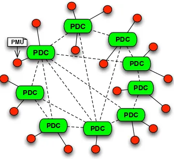
illustrates a setup of WAMS. PDCs and PMUs are connected via a communication network infrastructure to transmit real-time data. The system must meet the temporal requirements of the data transmission and task execution on PDCs and PMUs to provide a reliable service.
PDC
PDC
PDC
PDC
PDC PMU
PDC
PDC PDC
PDC
Figure 1.1: Wide-Area Monitoring System
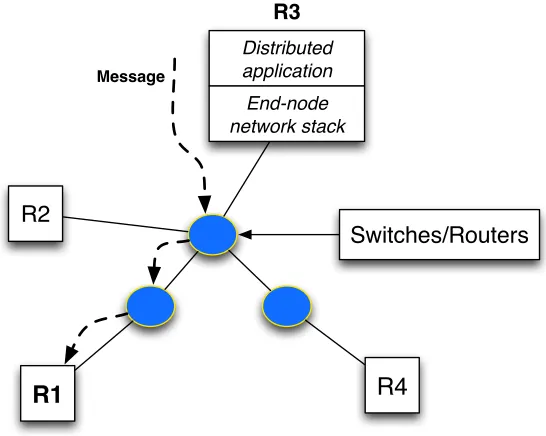
Fig. 1.2 depicts the interaction of components within this distributed real-time system. End nodes R1, R2, R3, and R4 are connected by the underlying network, which utilizes network switches/routers to transmit messages. A message sent by a distributed task on one end node needs to pass through multiple layers of the system to reach the task on another node. First, the distributed task in the application layer injects a message via the network stack implementation on the end node. Second, the message is forwarded by network devices to reach the destination node. Then, the message is received by the network stack on the destination node and relayed to the corresponding distributed task.
R1
R2
R4
Distributed application
End-node network stack
Switches/Routers
Message
R3
Figure 1.2: Distributed Systems Abstract
real-time systems with hard deadlines, a packet scheduler on network devices is required. This packet scheduler can prioritize packets according to their temporal requirements and avoid dropping them when network contention occurs. The focus of this work is to implement real-time schedulers on all layers to improve the predictability for distributed real-real-time systems.
1.3
Temporal Requirements
Real-time tasks can be executed periodically or sporadically. Periodic tasks have regular release times and sporadic tasks have irregular release times. The term job represents a release of a real-time task. This work assumes real-time tasks to be periodic. A periodic task has the following temporal properties:
1. P hase denotes the release time of the first job of the task.
2. P eriod denotes the inter-arrival time between two consecutive releases of the task.
3. W CET denotes the worst-case execution time of a job of the task,
4. Deadline denotes the time instance by which the job must be finished.
6. Response Time denotes the time difference between the release time and the time when the job is finished.
Periodic tasks pass messages to communicate with each other in a periodic manner. These messages can be organized as message flows. One message flow includes the periodic messages between two periodic tasks located on different end nodes. Similar to real-time tasks, a message flow has the following properties:
1. P eriod denotes the time interval that an end node transmits two consecutive messages from the same flow to the network.
2. Deadlinedenotes the time instance by when the message has to arrive at its destination node.
3. Relative Deadline denotes the time difference between the release time and the deadline of the message.
4. Sizedenotes the size of the packet that carries the message.
These properties of real-time tasks and message flows are utilized in the schedulability test to ensure that their deadline requirements can be met by the schedulers.
1.4
Contributions
This dissertation assesses if the end-to-end predictability for distributed real-time systems can be provided by controlling the behavior of different layers of the systems. The following are the major contributions in this document:
2. In Chapter 3, we present a hybrid EDF packet scheduler for real-time distribute systems to increase the predictability of packet scheduling on end nodes [49]. This work enhances the storage system by realizing the urgency (i.e., deadlines of requests) and scheduling these tasks accordingly. Employing EDF scheduling in distributed real-time systems has many challenges. First, the network layer of a resource has to notify the task scheduler about the deadlines of received messages. The randomness of interrupts due to such notifi-cations makes context switch costs unpredictable. Second, communication delay variances in a network increase the timing unpredictability of packets, e.g., when multiple resources transmit message bursts simultaneously. To address these challenges, we implement an EDF-based packet scheduler, which transmits packets considering event deadlines. Then, we employ bandwidth limitations on the transmission links of resources to decrease net-work contention and netnet-work delay variance. We evaluate this net-work on a cluster of nodes in a switched network environment resembling a distributed cyber-physical system to demonstrate the real-time capability of the hybrid scheduler.
3. In Chapter 4, we present a static routing algorithm and a packet scheduler on network devices to transmit real-time messages via the underlying networks [50]. First, the static routing algorithm derives forwarding paths for real-time packets to guarantee their hard deadlines. This algorithm employs a validation-based backtracking procedure, which con-siders both the demand of real-time message transmissions and the limitation of network resource capabilities. The algorithm can check whether this demand can be met on the network devices. Second, the packet scheduler transmits real-time messages according to our routing requirements. In addition, the packet scheduler guarantees that only pack-ets with no temporal requirements can be dropped when network contention occurs. We evaluate this work in a local cluster to demonstrate the feasibility and effectiveness of our static routing algorithm and packet scheduler.
1.5
Hypothesis
1. Unpredictability of transmission due to dropped packets when network contention occurs, which potentially increases the rate of deadline misses.
2. Coarse-grained quality of service support, which limits the capability of real-time systems.
3. Lack of support for temporal requirements when routing process is required to establish forwarding paths.
We attempt to extend the current network infrastructures to address these shortages in this dissertation. The hypothesis of this dissertation is as follows.
Distributed real-time systems can increase their predictability when the predictability of all
involved system layers (i.e., end-nodes and connecting network infrastructure) is increased. The
deployment of real-time task and packet schedulers provides a fine-grained support to temporal requirements of distributed real-time tasks on both end nodes and network devices to effectively
increase this predictability.
1.6
Organization
Chapter 2
A Real-time Distributed Hash Table
2.1
Introduction
The North American power grid uses Wide-Area Monitoring System (WAMS) technology to monitor and control the state of the power grid [45, 38]. WAMS increasingly relies on Phasor Measurement Units (PMUs), which are deployed to different geographic areas, e.g., the Eastern interconnection area, to collect real-time power monitoring data per area. These PMUs period-ically send the monitored data to a phasor data concentrator (PDC) via proprietary Internet backbones. The PDC monitors and optionally controls the state of the power grid on the ba-sis of the data. However, the current state-of-art monitoring architecture uses one centralized PDC to monitor all PMUs. As the number of PMUs is increasing extremely fast nowadays, the centralized PDC will soon become a bottleneck [12]. A straight-forward solution is to distribute multiple PDCs along with PMUs, where each PDC collects real-time data from only the part of PMUs that the PDC is in charge of. In this way, the PDC is not the bottleneck since the number of PMUs for each PDC could be limited and new PDCs could be deployed to manage new PMUs.
Our idea is to build a distributed hash table (DHT) on these distributed storage nodes to solve the first problem. Similar to a single node hash table, a DHT providesput(key, value) and get(key)API services to upper layer applications. In our DHT, the data of one PMU are not only stored in the PDC that manages the PMU, but also in other PDCs that keep redundant copies according to the distribution resulting from the hash function and redundancy strategy. DHTs are well suited for this problem due to their superior scalability, reliability, and performance over centralized or even tree-based hierarchical approaches. The performance of the service provided by some DHT algorithms, e.g., Chord [40] and CAN [52], decreases only insignificantly while the number of the nodes in an overlay network increases. However, there is a lack of research on real-time bounds for these DHT algorithms for end-to-end response times of requests. Timing analysis is the key to solve the second problem. On the basis of analysis, we could provide statistical upper bounds for request times. Without loss of generality, we use the term lookup request orrequest to represent either aput request or a get request, since the core functionality of DHT algorithms is to look up the node that is responsible for storing data associated with a given key.
It is difficult to analyze the time to serve a request without prior information of the workloads on the nodes in the DHT overlay network. However, in our research, requests follow a certain pattern, which makes the analysis concrete. For example, PMUs periodically send real-time data to PDCs [38], so that PDCs issue put requests periodically. At the same time, PDCs need to fetch data from other PDCs to monitor global power states and control the state of the entire power grid periodically. Using these patterns of requests, we design a real-time model to describe the system. Our problem is motivated by the power grid situation but our abstract real-time model provides a generic solution to analyze response time for real-time applications over network. We further apply queuing theory to stochastically analyze the time bounds for requests. Stochastic approaches may break with traditional views of real-time systems. However, cyber-physical systems rely on stock Ethernet networks with TCP/IP enhanced, so that new soft real-time models for different QoS notions, such as simplex models [10, 4], are warranted.
includes: 1) employing real-time executives on nodes, 2) abstracting a pattern of requests, and 3) using a stochastic model to analyze response time bounds under the cyclic executive and the given request pattern. The real-time executive is not limited to a cyclic executive. For example, we show that a prioritized extension can increase the probability of meeting deadlines for requests that have failed in their first time execution. This work, while originally motivated by novel control methods in the power grid, generically applies to distributed control of CPS real-time applications.
The rest of the paper is organized as follows. Section 2.2 presents the design and imple-mentation details of our real-time DHT. Section 2.3 presents our timing analysis and quality of service model. Section 2.4 presents the evaluation results. Section 2.5 presents the related work. Section 2.6 presents the conclusion and on-going part of our research.
2.2
Design and Implementation
Our real-time DHT uses the Chord algorithm to locate the node that stores a given data item. Let us first summarize the Chord algorithm and characterize the lookup request pattern (generically and specifically for PMU data requests). After that, we explain how our DHT implementation uses Chord and cyclic executives to serve these requests.
2.2.1 Chord
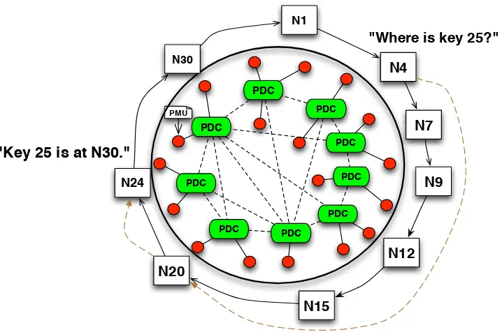
Given a particular key, the Chord protocol locates the node that the key maps to. Chord applies consistent hashing to assign keys to Chord nodes organized as a ring network overlay [40, 25]. The consistent hash uses a base hash function, such as SHA-1, to generate an identifier for each node by hashing the node’s IP address. When a lookup request is issued for a given key, the consistent hash uses the same hash function to encode the key. It then assigns the key to the first node on the ring whose identifier is equal to or follows the hash code of that key. This node is called the successor node of the key, or the target node of the key. Fig. 2.1 depicts an example of a Chord ring in the power grid context, which maps 9 PDCs onto the virtual nodes on the ring (labels in squares are their identifiers). As a result, PDCs issue requests to the Chord ring to periodically store and obtain PMU data from target PDCs. This solves the first problem that we have discussed in Section 2.1.
PDC
PDC
PDC
PDC PDC
PMU
PDC
PDC PDC
PDC
N4
N1
N7
N9
N12
N15 N20
N24
N30
"Where is key 25?"
"Key 25 is at N30."
Figure 2.1: PDC and Chord Ring Mapping Example
of the node is the target node of the given key. Consider Fig. 2.1. The starting nodeN4 needs to locate key 25 (i.e.,K25). By forwarding lookup messages along the circular list, N4 locates
N30 as the target node ofK25 via intermediate nodesN7, N9, N12, N15, N20, N24. However, the linear traversal requiresO(N) messages to find the successor node of a key, where N is the number of the nodes.
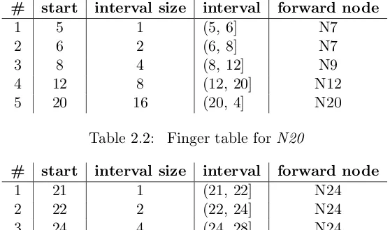
This linear algorithm is not scalable with increasing numbers of nodes. In order to reduce the number of intermediate nodes, Chord maintains a so-called finger table on each node, which acts as a soft routing table, to decide the next hop to forward lookup requests to. For example, assuming 5-bit numbers are used to represent node identifiers in Fig. 2.1, the finger table for N4 is in Table 2.1. The interval for the 5th finger is (20, 36], which is (20, 4] as the virtual nodes are organized as a ring (modulo 32). In general, a finger table has log(N) entries, where
N is the number of bits of node identifiers. For node k, the start of theithfinger table entry is
k+ 2i−1, the interval is (k+ 2i−1, k+ 2i], and the forward node is the successor of keyk+ 2i−1 (i.e., the beginning of the interval). Each entry in the table indicates one routing rule: the next hop for a given key is the forward node in that entry if the entry interval includes the key. For example, the next hop for K25 is N20 as25 is in (20, 4].
Table 2.1: Finger table forN4
# start interval size interval forward node
1 5 1 (5, 6] N7
2 6 2 (6, 8] N7
3 8 4 (8, 12] N9
4 12 8 (12, 20] N12
5 20 16 (20, 4] N20
Table 2.2: Finger table for N20
# start interval size interval forward node
1 21 1 (21, 22] N24
2 22 2 (22, 24] N24
3 24 4 (24, 28] N24
4 28 8 (28, 4] N30
5 4 16 (4, 20] N4
N20 according to its finger table (shown as the dotted line in Fig. 2.1). Next, N20 forwards
K25 to N24 according to N20’s finger table (depicted in Table 2.2). N24 considers itself the predecessor ofK25 sinceK25 is betweenN24 and its successorN30. Chord returns the successor N30 of the predecessorN24 as the target node ofK25. In this example, only two intermediate nodesN20 andN24 are required to locate K25 via the finger tables. In general, each message forwarding reduces the distance to the target node to at least half that of the previous distance on the ring. Thus, the number of intermediate nodes per request is at most log(N) with high probability [40], which is more scalable than the linear algorithm.
In addition to scalability, Chord tolerates high levels of churn in the distributed system. which makes it possible to provide PMU data with the possibility that some PDC nodes or network links have failed in the power grid environment. However, resilience analysis with real-time considerations is beyond the scope of this paper. Thus, our model in this paper derives the response times for requests assuming that nodes do not send messages in the background for resilience purpose.
2.2.2 The pattern of requests and jobs
together with the period of each task. Each node releases periodic tasks in the list to issue lookup requests. Once a request is issued, one job on each node on the way is required to be executed until the request is eventually served.
Jobs on the initial nodes are periodic, since they are driven by lists of periodic requests. However, jobs on the subsequent nodes are not necessarily periodic, since they are driven by the lookup messages sent by other nodes via the network. The network delay to transmit packets is not always constant, even one packet is enough to forward a request message as the length of PMU data is small in the power grid system. Thus, the pattern of these subsequent jobs depends on the node-to-node network delay. With different conditions of the network delay, we consider two models.
(1) In the first model, the network delay to transmit a lookup message is constant. Under this assumption, we use periodic tasks to handle messages sent by other nodes. For example, assume node A has a periodic PUT task τ1(0, T1, C1, D1). We use notation τ(φ, T, C, D) to
specify a periodic task τ, where φis its phase, T is the period, C is the worst case execution time per job, and D is the relative deadline. From the schedule table for the cyclic executive, the response times for the jobs of τ1 in a hyperperiod H are known [34]. Assume two jobs of
this task, J1,1 and J1,2, are in one hyperperiod on node A, with R1,1 and R1,2 as their release
times relative to the beginning of the hyperperiod and W1,1 and W1,2 as the response times,
respectively.
Let the network latency be the constantδ. The subsequent message of the jobJ1,1is sent to
node B at time R1,1+W1,1+δ. For a sequence of hyperperiods on node A, the jobs to handle
these subsequent messages on node B become a periodic task τ2(R1,1 +W1,1 +δ, H, C2, D2).
The period of the new task is H as one message ofJ1,1 is issued per hyperperiod. Similarly, jobs
to handle the messages ofJ1,2 become another periodic task τ3(R1,2+W1,2+δ, H, C2, D2) on
node B.
(2) In the second model, network delay may be variable, and its distribution can be mea-sured. We use aperiodic jobs to handle subsequent messages. Our DHT employs a cyclic ex-ecutive on each node to schedule the initial periodic jobs and subsequent aperiodic jobs, as discussed in the next section.
2.2.3 Job scheduling
Table 2.3: Types of Messages passed among nodes
Type 1 Parameters2 Description
PUT :key:value the initial put request to store (key:value). PUT DIRECT :ip:port:sid:key:value one node sends to the target node to store
(key:value). 3
PUT DONE :sid:ip:port the target node notifies sender of successfully handling the PUT DIRECT.
GET :key the initial get request to get the
value for the given key.
GET DIRECT :ip:port:sid:key one node sends to the target node to get the value.
GET DONE :sid:ip:port:value the target node sends the value back as the feed back of the GET DIRECT. GET FAILED :sid:ip:port the target node has no associated value. LOOKUP :hashcode:ip:port:sid the sub-lookup message. 4
DESTIN :hashcode:ip:port:sid similar to LOOKUP, but DESTIN message sends to the target node.
LOOKUP DONE :sid:ip:port the target node sends its address back to the initial node.
1 Message types for Chord fix finger and stabilize operations are omitted. 2 One message passed among the nodes consists of its type and the parameters,
e.g, PUT:PMU-001:15.
3 (ip:port) is the address of the node that sends the message. Receiver uses
it to locate the sender. sid is unique identifier.
4 Nodes use finger tables to determine the node to pass the LOOKUP to.
(ip:port) is the address of the request initial node.
Each node in our system employs a cyclic executive to schedule jobs using a single thread. The schedule table L(k) indicates which periodic jobs to execute at a specific frame k in a hyperperiod of F frames. L is calculated offline from the periodic tasks parameters [34]. Each node has a FIFO queue of released aperiodic jobs. The cyclic executive first executes periodic jobs in the current frame. It then executes the aperiodic jobs (up to a given maximum time allotment for aperiodic activity, similar to an aperiodic server). If the cyclic executive finishes all the aperiodic jobs in the queue before the end of the current frame, it waits for the next timer interrupt. Algorithm 1 depicts the work of the cyclic executive, wheref is the interval of each frame.
Data:L,aperiodic job queue Q,current job
1 Procedure SCHEDULE
2 current←0
3 setup timer to interrupt every f time, executeTIMER HANDLERwhen it interrupts
4 whiletrue do
5 current job←L(current) 6 current= (current+ 1)%F 7 if current job6=nil then 8 executecurrent job
9 markcurrent jobdone
10 end
11 whileQ is not empty do
12 current job←remove the head of Q 13 executecurrent job
14 markcurrent jobdone
15 end
16 current job←nil
17 wait for next timer interrupt 18 end
19 Procedure TIMER HANDLER
20 if current job6=nil and not done then 21 if current job is periodic then 22 mark thecurrent jobfailed 23 else
24 save state and pushcurrent jobback to the head ofQ
25 end
26 end
27 jump toLine4
Algorithm 1:Pseudocode for the cyclic executive
2.2.4 Real-time DHT
Our real-time DHT is a combination of Chord and cyclic executive to provide predictable response times for requests following the request pattern. Our DHT adopts Chord’s algorithm to locate the target node for a given key. On the basis of Chord, our DHT provides two operations: get(key)andput(key, value), which obtains the paired value with a given key and puts one pair onto a target node, respectively. Table 2.3 describes the types of messages exchanged among nodes. Algorithms 2 and 3 depicts the actions for a node to handle these messages. We have omitted the details of failure recovery messages such as fix finger and stabilize in Chord, also implemented as messages in our DHT.node.operation(parameters) indicates that the operation with given parameters is executed on the remote node, implemented by sending a corresponding message to this node.
As an example, in order to serve the periodic task to get K25 on node N4 in Fig. 2.1, the cyclic executive on N4 schedules a periodic job GET periodically, which sends a LOOKUP message to N20. N20 then sends a LOOKUP message to N24. N24 then sends a DESTIN message toN30 since it determines thatN30 is the target node forK25.N30 sendsLOOKUP -DONE back to the initial nodeN4. Our DHT stores the request detail in a buffer on the initial node and uses a unique identifier (sid) embedded in messages to identify this request. When N4 receives theLOOKUP DONE message from the target node, it releases an aperiodic job to obtain the request detail from the buffer and continue the request by sending GET DIRECT to the target nodeN30 as depicted in the pseudocode.N30 returns the value toN4 by sending a GET DONE message back to N4. Now, N4 removes the request detail from the buffer and the request is completed.
2.3
Analysis
As a decentralized distributed storage system, the nodes in our DHT work independently. In this section, we first explain the model that we use to analyze the response times of jobs on a single node. Then, we aggregate them to bound the end-to-end time for all requests.
2.3.1 Job response time on a single node
1 Procedure GET(key) and PUT(key, value)
2 sid← unique request identifier 3 code←hashcode(key)
4 address←ip and port of this node 5 store the request in the buffer 6 executeLOOKUP(address, sid, code)
7 Procedure LOOKUP(initial-node, sid, hashcode)
8 next← next node for the lookup in the finger table 9 if next=target nodethen
10 next.DESTIN(initial-node, sid, hashcode)
11 else
12 next.LOOKUP(initial-node, sid, hashcode)
13 end
14 Procedure DESTIN(initial-node, sid, hashcode)
15 address←ip and port of this node 16 initial-node.LOOKUP DONE(address, sid)
17 Procedure LOOKUP DONE(target-node, sid)
18 request← find buffered request using sid 19 if request=get then
20 target-node.GET DIRECT(initial-node, sid, request.key)
21 else if request=putthen
22 target-node.PUT DIRECT(initial-node, sid, request.key, request.value)
23 else if request=f ix f inger then 24 update the finger table
25 end
Algorithm 2:Pseudocode for message handling jobs (1)
the aperiodic job queue is not empty. Since aperiodic jobs are released when the node receives messages from other nodes, we model the release pattern of aperiodic jobs as a homogeneous Poisson process with 2msas the average inter-arrival time. The execution time is 0.4msfor all aperiodic jobs. The problem is to analyze response times of these aperiodic jobs. The response time of an aperiodic job in our model consists of the time waiting for the receiving task to move its message to the aperiodic queue, the time waiting for the executive to execute the job, and the execution time of the job.
1 Procedure GET DIRECT(initial-node, sid, key)
2 address←ip and port of this node
3 value← find value forkey in local storage 4 if value=nil then
5 initial-node.GET FAILED(address, sid)
6 else
7 initial-node.GET DONE(address, sid, value)
8 end
9 Procedure PUT DIRECT(initial-node, sid, key, value)
10 address←ip and port of this node 11 store the pair to local storage 12 initial-node.PUT DONE (address, sid)
13 Procedure PUT DONE, GET DONE, GET FAILED
14 execute the associated operation
Algorithm 3:Pseudocode for message handling jobs (2)
Formally, Table 2.4 includes the notation we use to describe our model. We also use the same notation without the subscript for the vector of all values. For example,U is (U0, U1, . . . , UK),
C is (C0, C1, . . . , CM). In the table, C is obtained by measurement from the implementation;
H, K, ν, U are known from the schedule table; M is defined in our DHT algorithm. We explain
λin detail in Section 2.3.2.
Given a time interval of length x and arrivalsg in that interval, the total execution time of aperiodic jobs E(x, g) can be calculated with Equation 2.1. Without loss of generality, we use notationE and E(x) to represent E(x, g).
E(x, g) =
M X
i=1
Ci∗gi with probability M Y
i=1
P(gi, λi, x) (2.1)
We further defineAp as the time available to execute aperiodic jobs in time interval (ν0, νp+1).
Ap = p X
i=0
(1−Ui)∗(νi+1−νi),0≤p≤K. (2.2)
However, the executive executes aperiodic jobs only when periodic jobs are finished in a frame. We define W(i, E) as the response time for an aperiodic job workload E if these jobs are scheduled after theith receiving job. For 1≤i≤K, W(i, E) is a function ofE calculated from the schedule table in three cases:
(1) If E ≤Ai−Ai−1, which means the executive can use the aperiodic job quota between
Table 2.4: Notation
Notation Meaning
H hyperperiod
K number of receiving jobs in one hyperperiod
νi time when theith receiving job is scheduled1,2
Ui utilization of periodic jobs in time interval (νi, νi+1)
M number of different types of aperiodic jobs
λi average arrival rate of the ith type aperiodic jobs
Ci worst case execution time of theith type aperiodic jobs
gi number of arrivals of ith aperiodic job
E(x, g) total execution time
for aperiodic jobs that arrive in time interval of lengthx W(i, E) response time for aperiodic jobs
if they are scheduled afterith receiving job
P(n, λ, x) probability ofn arrivals in time interval of length x, when arrival is a Poisson process with rate λ
1 ν
i are relative to the beginning of the current hyperperiod. 2 For convenience,ν
0is defined as the beginning of a hyperperiod,νK+1
is defined as the beginning of next hyperperiod.
table to calculateW(i, E).
(2) If ∃p ∈ [i+ 1, K] so that E ∈ (Ap−1−Ai−1, Ap −Ai−1], which means the executive
utilizes all the aperiodic job quota between (νi, νp) to execute the workload and finishes the
workload at a time between (νp, νp+1), then W(i, E) =νp−νi+W(p, E−Ap−1+Ai−1).
(3) In the last case, the workload is finished in the next hyperperiod. W(i, E) becomes
H −νi +W(0, E −AK +Ai−1). W(0, E) means to use the aperiodic quota before the first
receiving job to execute the workload. If the first receiving job is scheduled at the beginning of the hyperperiod, this value is the same asW(1, E). In addition, we require that any workload finishes before the end of the next hyperperiod. This is accomplished by analyzing the timing of receiving jobs and ensures that the aperiodic job queue is in the same state at the beginning of each hyperperiod, i.e., no workload accumulates from previous hyperperiods except the last hyperperiod.
Let us assume an aperiodic job J of execution time Cm arrives at time t relative to the
beginning of the current hyperperiod. Let p+ 1 be the index of the receiving job such that
t ∈ [νp, νp+1). We also assume that any aperiodic job that arrives in this period is put into
the aperiodic job queue by this receiving job. Then, we derive the response time of this job in different cases.
in the current frame cannot be finished before νp+1. Equation 2.3 is the formal condition for
this case, in whichHLW is the leftover workload from the previous hyperperiod.
HLW +E(νp)−Ap >0 (2.3)
In this case, the executive has to first finish this leftover workload, then any aperiodic jobs that arrive in the time period [νp, t), which isE(t−νp), before executing jobJ. As a result, the total
response time of jobJ is the time to wait for the next receiving job atνp+1, which putsJ into
the aperiodic queue, and the time to execute aperiodic job workloadLW(νp) +E(t−νp) +Cm,
which isW(p+ 1, HLW+E(t)−Ap+Cm), after the (p+ 1)th receiving job. The response time
of J is expressed in Equation 2.4.
R(Cm, t) =
(νp+1−t) +
W(p+ 1, HLW+E(t)−Ap+Cm)
(2.4)
(2) In the second case, the periodic jobs that are left over from the previous hyperperiod and arrive before νp can be finished before νp+1; the formal condition and the response time
are given by Equations 2.5 and 2.6, respectively.
HLW +E(νp)≤Ap (2.5)
R(Cm, t) = (νp+1−t) +W(p+ 1, E(t−νp) +Cm) (2.6)
The hyperperiod leftover workload HLW is modeled as follows. Consider three continuous hyperperiod, H1, H2, H3. The leftover workload from H2 consists of two parts. The first part,
E(H −νK), is the aperiodic jobs that arrive after the last receiving job in H2, as these jobs
can only be scheduled by the first receiving job in H3. The second part,E(H+νK)−2AK+1,
is the jobs that arrive in H1 and before the last receiving job in H2 which have not been
scheduled in all the aperiodic allotment in H1 and H2. We construct a distribution for HLW
in this way. In addition, more previous hyperperiods considered results in more stable model for HLW. However, our evaluation shows that two previous hyperperiods is sufficient for the request patterns.
Now we have the stochastic model R(Cm, t) for the response time of an aperiodic job of
execution timeCm that arrives at a specific timet. By samplingt in one hyperperiod, we have
2.3.2 End-to-end response time analysis
We aggregate the single node response times and network delays to transmit messages for the end-to-end response time of requests. The response time of any request consists of four parts: (1) the response time of the initial periodic job; this value is known by the schedule table; (2) the total response time of jobs to handle subsequent lookup messages on at most logN
nodes with high probability [40], where N is the number of nodes; (3) the response time of aperiodic jobs to handle LOOKUP DONE, and the final pair of messages, e.g., PUT DIRECT and PUT DONE; (4) the total network delays to transmit these messages. We use a value δ
based on measurement for the network delay, where P(network delay ≤ δ) ≥ T, for a given thresholdT.
To use the single node response time model, we need to know the values of the model parameters of Table 2.4. With the above details on requests, we can obtain H, K, v, U from the schedule table. λ is defined as follows: let T be the period of the initial request on each node, then NT new requests arrive at our DHT in one time unit, and each request at most logN
subsequent lookup messages. Let us assume that hash codes of nodes and keys are randomly located on the Chord ring, which is of high probability with the SHA-1 hashing algorithm. Then each node receives logNT lookup messages in one time unit. The arrival rate of LOOKUP and DESTIN messages is logNT . In addition, each request eventually generates one LOOKUP DONE message and one final pair of messages, so for these messages the arrive rate is T1.
2.3.3 Quality of service
We define quality of service (QoS) as the probability that our real-time DHT can guarantee requests to be finished before their deadlines. Formally, given the relative deadline D of a request, we use the stochastic modelR(Cm, t) for single node response times and the aggregation
model for end-to-end response times to derive the probability that the end-to-end response time of the request is equal or less than D. In this section, we apply the formula in our model step by step to explain how to derive this probability in practice.
The probability density function ρ(d, Cm) is defined as the probability that the single node
response time of a job with execution time Cm is d. We first derive the conditional density
function ρ(d, Cm|t), which is the probability under the condition that the job arrives at time
t, i.e., the probability thatR(Cm, t) =d. Then, we apply the law of total probability to derive
ρ(d, Cm). The conditional density function ρ(d, Cm|t) is represented as a table of pairs π(ρ, d),
where ρ is the probability that an aperiodic job finishes with response time d. We apply the algorithms described in Section 2.3.1 to build this table as follows. Let p+ 1 be the index of the receiving job such that t∈[νp, νp+1).
probability χ that condition HLW +E(νp, g) ≤Ap holds. To calculate χ, we enumerate job
arrival vectors g that have significant probabilities in time (0, νp) according to the Poisson
distribution, and use Equation 2.1 to calculate the workload E(νp, g) for each g. The term
significant probability means any probability that is larger than a given threshold, e.g., 0.0001%. Since the values ofHLW andE(νp, g) are independent, the probability of a specific pair ofHLW
and arrival vectorg is given by simply their multiplications. As a result, we build a condition table CT(g, ρ), in which each row represents a pair of vector g, which consists of the numbers of aperiodic job arrivals in time interval (0, νp) under the conditionHLW+E(νp, g)≤Ap, and
the corresponding probability ρ for that arrival vector. Then, χ=P
ρ is the total probability for that condition.
(2) Build probability density tableπ2(ρ, d) for response times of aperiodic jobs under
condi-tionHLW+E(νp)≤Ap. In this case, we enumerate job arrival vectorsg that have significant
probabilities in time (0, t−νp) according to the Poisson distribution. and use Equation 2.1
to calculate its workload, use Equation 2.6 to calculate its response time for each g. Each job arrival vector generates one row in density tableπ2.
(3) Build probability density table π3(ρ, d) for response times of aperiodic jobs under
con-dition HLW +E(νp) > Ap. We enumerate job arrival vectors g that have significant
proba-bilities in time (0, t) according to the Poisson distribution, and use Equation 2.4 to calculate response times. Since time interval (0, t) includes (0, νp), arrival vectors that are in condition
table CT must be excluded from π3, because rows in CT only represent arrivals that results
in HLW +E(νp) ≤ Ap. We normalize the probabilities of the remaining rows. By
normaliz-ing, we mean multiplying each probability by a same constant factor, so that the sum of the probabilities is 1.
(4) We merge the rows in these two density tables to build the final table for the conditional density function. Before merging, we need to multiply every probability in table π2 by the
weight χ, which indicates the probability that rows in table π2 are valid. For the same reason,
every probability in table π3 is multiplied by (1−χ).
Now, we apply the law of total probability to derive ρ(d, Cm) from the conditional density
functions by samplingtin [0, H). The conditional density tables for all samples are merged into a final density tableQ
(ρ, d). The samples are uniformly distributed in [0, H) so that conditional density tables have the same weight during the merge process. After normalization, tableQ
is the single node response time density functionρ(d, Cm).
We apply the aggregation rule described in Section 2.3.2 to derive the end-to-end response time density function on the basis ofρ(d, Cm). According to the rule, end-to-end response time
1 Procedure UNIQUE(π)
2 πdes←empty table
3 foreach row (ρ, d) in π do
4 if row (ρold, d) exists in πdes then 5 ρold←ρold+ρ
6 else
7 add row (ρ, d) toπdes
8 end
9 end
10 returnπdes
11 Procedure SUM(π1, π2)
12 π3 ←empty table
13 foreach row (ρ1, d1) in π1 do
14 foreach row (ρ2, d2) in π2 do
15 add row (ρ1∗ρ2, d1+d2) toπ3
16 end
17 end
18 returnUNIQUE(π3)
Algorithm 4:Density tables operations
tablesπ1 andπ2 as in Algorithm 4. The resulting density table has one row (ρ1∗ρ2, d1+d2) for
each pair of rows (ρ1, d1) and (ρ2, d2) from tableπ1 and π2, respectively. That is, each row in
the result represents one sum of two response times from the two tables and the probability of the aggregated response times. The density function of the total response time for (logN+ 3) aperiodic jobs is calculated as Equation 2.7 (SU M on allπi), where πi is the density function
for theith job.
ρ(d) =
logN+3 X
i=1
πi (2.7)
The maximum number of rows in density tableρ(d) is 2(logN+3)Hω, where 2His the maximum response time of single node jobs, and ω is the sample rate for arrival time t that we use to calculate each density table.
Let us return to the QoS metric, i.e., the probability that a request can be served within a given deadline D. We first reduce D by fixed value ∆, which includes the response time for the initial periodic job and network delays (logN+ 3)δ. Then, we aggregate rows in the density functionρ(d) to calculate this probability P(D−∆).
P(D−∆) = X
(ρi,di)∈ρ(d),di≤D−∆
2.4
Evaluation
In this section, we evaluate our real-time DHT on a local cluster with 2000 cores over 120 nodes. Each node features a 2-way SMP with AMD Opteron 6128 (Magny Core) processors and 8 cores per socket (16 cores per node). Each node has 32GB DRAM and Gigabit Ethernet (utilized in this study) as well as Infiniband Interconnect (not used here). We apply workloads of different intensity according to the needs of the power grid control system on different numbers of nodes (16 nodes are utilized in our experiments), which act like PDCs. The nodes are not synchronized to each other relative to their start of hyperperiods as such synchronization would be hard to maintain in a distributed system. We design experiments for different intensity of workloads and then collect single-node and end-to-end response times of requests in each experiment. The intensity of a workload is quantified by the system utilization under that workload. The utilization is determined by the number of periodic lookup requests and other periodic power control related computations. The lookup keys have less effect on the workload and statistic results as long as they are evenly stored on the nodes, which has high probability in Chord. In addition, the utilization of aperiodic jobs is determined by the number of nodes in the system. The number of messages passing between nodes increases logarithmically with the number of nodes, which results in an increase in the total number of aperiodic jobs. We compare the experimental results with the results given by our stochastic model for each workload.
In the third part of this section, we give experimental results of our extended real-time DHT, in which the cyclic executive schedules aperiodic jobs based on the priorities of requests. The result shows that most of the requests that have tight deadlines can be finished at the second trial under the condition that the executive did not finish the request at the first time.
2.4.1 Low workload
In this experiment, we implement workloads of low utilizations for the cyclic executive to schedule. In detail, one hyperperiod (30ms) contains three frames of 10ms, each with a periodic followed by an aperiodic set of jobs. The periodic jobs include the receiving job for each frame and the following put/get jobs: In frame 1, each node schedules a put request followed by a
0 2 4 6 8 10 12 14 16 18 20 22 24
0 2 4 6 8 10 12 14 16 18 20 22 24 26 28 30
Response Time (ms)
Relative Arrival Time (ms)
Measured Modeled Average Modeled Max
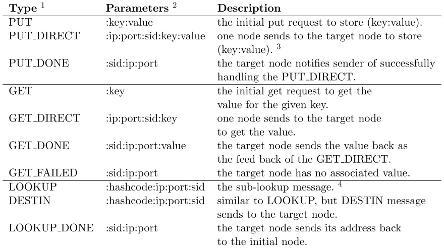
Figure 2.2: Low-workload Single-node Response Times (4 nodes)
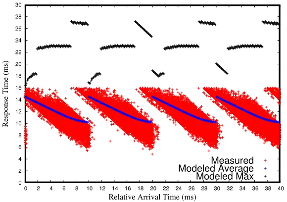
Results are plotted over 3,000 hyperperiods. Fig. 2.2 depicts the single-node response times comparison. The red dots in the figure are measured response times of jobs. Since our stochastic model derives a distribution of response times for jobs arriving at every time instance relative to the hyperperiod, we depict the mathematical expectation and the maximum value for each time instance, which are depicted as blue and black lines in the figure, respectively. The figure shows that messages sent at the beginning of each frame experience longer delays before they are handled by corresponding aperiodic jobs with proportionally higher response times. The reason for this is that these messages spend more time waiting for the execution of the next receiving job so that their aperiodic jobs can be scheduled. The modeled average times (blue) follow a proportionally decaying curve delimited by the respective periodic workload of a frame (4ms) plus the frame size (10ms) as the upper bound (left side) and just the periodic workload as the lower bound (right side). The figure shows that the measured times (red) closely match this curve as the average response time for most of the arrival times.
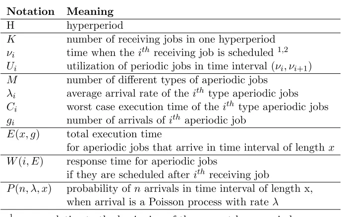
Fig. 2.3 depicts the cumulative distributions of single-node response times for aperiodic jobs. The figure shows that 99.3% of the aperiodic jobs finish within the next frame after they are released under this workload, i.e., their response times are bounded by 14.4ms. Our model predicts that 97.8% of aperiodic jobs are finished within the 14.4ms deadline, which is a good match. In addition, for most of the response times in the figure, our model predicts that a smaller fraction of aperiodic jobs is finished within the response times than the fraction in the experimental data, as the blue curve for modeled response times is below the red curve, i.e., the former effectively provides a lower bound for the latter. This indicates that our model is conservative for low workloads.
0 5 10 15 20 25 30 35 40 45 50 55 60 65 70 75 80 85 90 95 100
0 2 4 6 8 10 12 14 16 18 20
Cumulative Distribution Function
Response Time (ms)
Modeled Average Measured
Figure 2.3: Low-workload Single-node Response Times Distribution (4 nodes)
0 5 10 15 20 25 30 35 40 45 50 55 60 65 70 75 80 85 90 95 100
20 30 40 50 60 70 80 90 100 110 120
Cumulative Distribution Function
Response Time (ms)
Modeled Average (4 nodes) Modeled Average (8 nodes) Measured (4 nodes) Measured (8 nodes)
Figure 2.4: Low-workload End-to-end Response Times Distribution
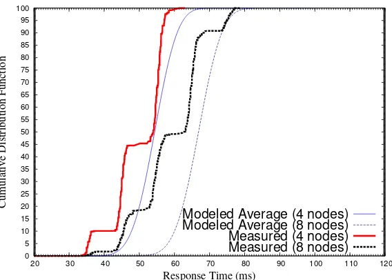
implementation sends a LOOKUP DONE message to itself directly. Our QoS model considers the worst case where log(N) nodes are required, which provides an upper bound on response times given a specific probability. In addition, this figure shows that our QoS model is conser-vative. For example, 99.9% of the requests are served within 62msin the experiment, while our model indicates 93.9% coverage for that response time.
In addition, we evaluate our model with the same request pattern with 8 DHT nodes. The system utilization becomes 72% as the utilization for aperiodic jobs increases because of the additional nodes in the DHT. Fig. 2.4 (dotted lines) depicts the cumulative distributions of end-to-end response times for requests. Four clusters of response times are shown in this figure (the base value is considered larger between 40ms and 45ms as the utilization has increased). One more intermediate node is contacted for a fraction of requests compared to the previous experiment with 4 DHT nodes.
2.4.2 High workload
0 2 4 6 8 10 12 14 16 18 20 22 24 26 28 30
0 2 4 6 8 10 12 14 16 18 20 22 24 26 28 30 32 34 36 38 40
Response Time (ms)
Relative Arrival Time (ms)
Measured Modeled Average Modeled Max
Figure 2.5: High-workload Single-node Response Times (8 nodes)
Fig. 2.5 depicts the single-node response times comparison. The red dots in the figure depict measured response times of jobs. The blue and black lines are the mathematical expectation and maximum response times for each sample instance given by our model, respectively. Compared with Fig. 2.2, a part of the red area at the end of each frame, e.g., between 8ms to 10ms for the first frame, moves up indicating response times larger than 14.4ms. This is due to a larger fraction of aperiodic jobs during these time interval being scheduled after the next frame (i.e., in the third frame), due to the increase of system utilization. Our model also shows this trend as the tails of blue lines curve up slightly. Figures 2.6 and 2.7 depict the cumulative distributions of single-node and end-to-end response times under this workload, respectively. Compared with Figures 2.3 and 2.4, the curves for higher utilization move to the right. This suggests larger response times. Our model provides upper bound on response times of 99.9% of all requests. Fig. 2.7 (dotted lines) also depicts the cumulative distribution of end-to-end response times of requests running on 16 DHT nodes. Our model also gives reliable results for this case, as the curves for the experimental data are slightly above the curves of our model.
These experiments demonstrate that a stochastic model can result in highly reliable response times bounds, where the probability of timely completion can be treated as a quality of service (QoS) property under our model.
2.4.3 Prioritized queue extension
0 5 10 15 20 25 30 35 40 45 50 55 60 65 70 75 80 85 90 95 100
0 2 4 6 8 10 12 14 16 18 20
Cumulative Distribution Function
Response Time (ms)
Modeled Average Measured
Figure 2.6: High-workload Single-node Response Times Distribution (8 nodes)
compare the results with that of the real-time DHT without prioritized queue for the low workload executed on 4 DHT nodes.
In this extension, the system assigns the lowest priority to jobs of requests that are released for the first time and sets a timeout at their deadline. If the system fails to complete a request before its deadline, it increases the priority of its next job release until that request is served before its deadline. To implement this, all the messages for a request inherit the maximum remaining response time, which is initially the relative deadline, to indicate the time left for that request to complete. This time is reduced by the single node response time (when the aperiodic job for that request is finished) plus the network delay δ if request is forwarded to the next node. When a node receives a message that has no remaining response time, the node simply drops the message instead of putting it onto aperiodic job queues. Cyclic executives always schedule aperiodic jobs with higher priority first (FCFS for the jobs of same priority).
In the experiment, we set the relative deadline of requests to 55ms, which is the duration within which half of the requests with two intermediate nodes can be served.
0 5 10 15 20 25 30 35 40 45 50 55 60 65 70 75 80 85 90 95 100
20 30 40 50 60 70 80 90 100 110 120
Cumulative Distribution Function
Response Time (ms)
Modeled Average (8 nodes) Modeled Average (16 nodes) Measured (8 nodes) Measured (16 nodes)
Figure 2.7: High-workload End-to-end Response Times Distribution
50ms. In addition, requests that have response times in the same cluster (e.g., centered around 45ms) could have larger numbers of intermediate nodes (hops) in the prioritized implementation since prioritized requests have smaller response times per sub-request job.
2.5
Related work
Distributed hash tables are well known for their performance and scalability for looking up the node that stores a particular piece of data in a distributed environment. Many existing DHTs use the number of nodes involved in one lookup request as a metric to measure performance. For example, Chord and Pastry requireO(logN) node traversals usingO(logN) routing tables to locate the target node for the given data in aN-nodes network [40, 56], while D1HT [39] and ZHT [32] requires a single node traversal of the expense ofO(N) routing tables. However, this level of performance analysis is not suited for real-time applications, as these applications require detailed timing information to guarantee time bounds on lookup requests. In our research, we focus on analyzing response times of requests by modeling the pattern of job executions on the nodes.
0 5 10 15 20 25 30 35 40 45 50 55 60 65 70 75 80 85 90 95 100
20 30 40 50 60 70 80
Cumulative Distribution Function
Response Time (ms)
FIFO Queue Prioritized Queue
Figure 2.8: End-to-end Response Times Distribution Comparison
state monitoring as it is more scalable in the numbers of PDCs and PMUs.
In our timing analysis model, we assume that node-to-node network latency is bounded. Much of prior research changes the OSI model to smooth packet streams so as to guarantee time bounds on communication between nodes in switched Ethernet [30, 14]. Software-defined networks (SDN), which allow administrators to control traffic flows, are also suited to control the network delay in a private network [36]. Distributed power grid control nodes are spread in a wide area, but use a proprietary Internet backbone to communicate with each other. Thus, it is feasible to employ SDN technologies to guarantee network delay bounds in a power grid environment [7].
2.6
Conclusion
the requests follow our pattern. Our evaluation shows that our model is suited to provide an upper bound on response times and that a prioritized extension can increase the probability of meeting deadlines for subsequent requests.
Chapter 3
Hybrid EDF Packet Scheduling for
Real-Time Distributed Systems
3.1
Introduction
When computational resource elements in a cyber-physical system are involved in the handling of events, understanding and controlling the scheduling algorithms on these resource elements become an essential part in order to make them collaborate to meet the deadlines of events. Our previous work has deployed a real-time distributed hash table in which each node employs a cyclic executive to schedule jobs that process data request events with probabilistic deadlines, which are resolved from a hash table [47]. However, cyclic executives are static schedulers with limited support for real-time systems where jobs have to be prioritized according to their urgency. Compared to static schedulers, EDF always schedules the job with earliest deadline first and has a utilization bound of 100% on a preemptive uniprocessor system [34, 33]. In theory, two major assumptions have to be fulfilled in real-time systems in order to achieve this utilization bound. First, the scheduler has to know the deadlines of all jobs in the system, so it can always schedule the job with the shortest deadline. Second, the cost of a context switch between different jobs is ignorable. To satisfy the second assumption, not only the cost of a single context switch, but also the number of context switches must be ignorable. This constrains the number of job releases in a period of time. Employing EDF schedulers in such a distributed system raises significant challenges considering the difficulty of meeting these assumptions in a cyber-physical system in which computational resource elements (i.e., nodes) communicate with each other by message passing.
until the job scheduler explicitly receives these messages and releases corresponding jobs to process them. The delays between the arrival and reception of messages provide a limitation on the capability of the job scheduler in terms of awareness of the deadlines of all current jobs on the node. One possible solution to address this problem is to let the operating system interrupt the job scheduler whenever a new message arrives at the node. In this way, the scheduler can always accept new messages at their arrival time so that it knows the deadlines of all current jobs. However, this may result in an unpredictable cost of switching between the job execution context and the interruption handling context that receives messages.
To address this problem, we combine a periodic message receiving task with the EDF sched-uler. This receiving task accepts messages from the system network buffer and releases corre-sponding jobs into job waiting queues of the EDF scheduler. Considering the fact that message jobs can only be released when the receiving task is executing, this design makes the scheduler partial-EDF because of the aforementioned delays. However, it increases the predictability of the system in terms of temporal properties including period, worst case execution time, and relative deadline of the receiving task, which also makes context switch cost more predictable. In addition, our partial-EDF adopts a periodic message sending task to regulate the messages sent by events so that the inter-transmission time of messages has a lower bound. We have theoretically studied the impact of the temporal properties of these transmission tasks on the schedulability of partial-EDF.
The second challenge is relevant to the deadlines carried in event messages. Since clocks of nodes in cyber-physical systems are not synchronized globally considering the cost of global clock synchronization [28], deadlines carried in messages sent by different nodes lose their signif-icance when these messages arrive at a node. To address this problem, our scheduler maintains a time-difference table on each node consisting of the clock difference between the senders and this receiving node. Hence, the deadlines carried in messages can be adjusted to the local time based on the information in this time-difference table. Thus, the EDF order of jobs can be main-tained. These time-difference tables are built based on the Network Time Protocol (NTP) [37], and they are periodically updated so that clock drifts over time can be tolerated.
in two ways. First, we propose an EDF-based packet scheduler that works on the system network layer on end nodes to transmit packets in EDF order. Second, since network congestion increases the variance of the network delay especially in communication-intensive cyber-physical systems (considering the fact that multiple nodes may drop messages onto the network simultaneously and that bursty messages may increase the packet queuing delay on intermediate network devices, which may require retransmission of message by end nodes), we employ a bandwidth sharing policy on end nodes to control the data burstiness in order to bound the worst-case network delay of message transmission. This is essentially a network resource sharing problem. In terms of resource sharing among parallel computation units, past research has focused on shaping the resource access by all units into well defined patterns. These units collaborate to reduce the variance of resource access costs. E.g., MemGuard [63] shapes memory accesses by each core in modern multi-core platforms in order to share memory bandwidth in a controlled way so that the memory access latency is bounded. D-NoC [13] shapes the data transferred by each node on the chip with a (σ, ρ) regulator [11] to provide a guaranteed latency of data transferred to the processor. We have implemented our bandwidth sharing policy based on a traffic control mechanism integrated into Linux to regulate the data dropped onto the network on each distributed node.
To demonstrate the feasibility and capability of our partial-EDF job scheduler, the EDF-based packet scheduler and the bandwidth sharing policy, , we integrated them into our previous real-time distributed hash table (DHT) that only provides probabilistic deadlines [47]. The new real-time distributed system still utilizes a DHT [40] to manage participating storage nodes and to forward messages between these nodes so that data requests are met. However, each participating node employs our partial-EDF job scheduler (instead of the cyclic executive in our previous paper) to schedule data request jobs at the application level. Furthermore, each node employs our EDF-based packet scheduler to send packets in EDF order at the system network level. In addition, all participating nodes follow our bandwidth sharing policy to increase the predictability of network delay. We evaluated our system on a cluster of nodes in a switched network environment.