University of Windsor University of Windsor
Scholarship at UWindsor
Scholarship at UWindsor
Electronic Theses and Dissertations Theses, Dissertations, and Major Papers
2011
Evaluation of Implicit and Explicit Methods of Uncertainty
Evaluation of Implicit and Explicit Methods of Uncertainty
Analysis on a Hydrological Modeling
Analysis on a Hydrological Modeling
Arpana Rani Datta University of Windsor
Follow this and additional works at: https://scholar.uwindsor.ca/etd
Recommended Citation Recommended Citation
Datta, Arpana Rani, "Evaluation of Implicit and Explicit Methods of Uncertainty Analysis on a Hydrological Modeling" (2011). Electronic Theses and Dissertations. 5397.
https://scholar.uwindsor.ca/etd/5397
This online database contains the full-text of PhD dissertations and Masters’ theses of University of Windsor students from 1954 forward. These documents are made available for personal study and research purposes only, in accordance with the Canadian Copyright Act and the Creative Commons license—CC BY-NC-ND (Attribution, Non-Commercial, No Derivative Works). Under this license, works must always be attributed to the copyright holder (original author), cannot be used for any commercial purposes, and may not be altered. Any other use would require the permission of the copyright holder. Students may inquire about withdrawing their dissertation and/or thesis from this database. For additional inquiries, please contact the repository administrator via email
Evaluation of Implicit and Explicit Methods of Uncertainty Analysis on a Hydrological Modeling
by
Arpana Rani Datta
A Dissertation
Submitted to the Faculty of Graduate Studies through Civil Engineering
in Partial Fulfillment of the Requirements for the Degree of Doctor of Philosophy at the
University of Windsor
Windsor, Ontario, Canada
2011
© 2011 Arpana Rani Datta
Evaluation of Implicit and Explicit Methods of Uncertainty Analysis on a Hydrological Modeling
by
Arpana Rani Datta
APPROVED BY:
______________________________________________ Dr. Raghavan Srinivasan, External Examiner
Texas A&M University
______________________________________________ Dr. Ram Balachandar
Department of Civil and Environmental Engineering
______________________________________________ Dr. Abdul-Fattah Asfour
Department of Civil and Environmental Engineering
______________________________________________ Dr. Ronald Barron
Department of Mathematics and Statistics
______________________________________________ Dr. Tirupati Bolisetti, Advisor
Department of Civil and Environmental Engineering
______________________________________________ Dr. Henry Hu, Chair of Defense
Department of Mechanical, Automotive and Materials Engineering
iii
DECLARATION OF CO-AUTHORSHIP/ PREVIOUS PUBLICATION
I hereby declare that this thesis incorporates the outcome of a research carried out by the
author under the supervision of Dr. Tirupati Bolisetti. The key ideas, experimental
designs, data analysis and interpretation, were performed by the author, and the
contributions of the co-authors was primarily through the provision of supervision.
I am aware of the University of Windsor Senate Policy on Authorship and I certify that I
have properly acknowledged the contribution of other researchers to my thesis, and have
obtained written permission from each of the co-author(s) to include the above
material(s) in my thesis.
I certify that, with the above qualification, this thesis, and the research to which it refers,
is the product of my own work.
Based on the research work, the following two papers have been submitted for
publication in peer reviewed journals:
Thesis Chapter Title of paper Publication status
Chapter 4 Estimation of model parameters and assessment of
uncertainty in a distributed hydrological model using
Bayesian approach, submitted to Journal of Hydrology
Under Review
Chapter 5 Quantifying parameter and predictive uncertainties in
distributed hydrological modeling considering input
uncertainty, submitted to Journal of Hydrology
iv
I certify that, to the best of my knowledge, my thesis does not infringe upon anyone‘s
copyright nor violate any proprietary rights and that any ideas, techniques, quotations, or
any other material from the work of other people included in my thesis, published or
otherwise, are fully acknowledged in accordance with the standard referencing practices.
I declare that this is a true copy of my thesis, including any final revisions, as approved
by my thesis committee and the Graduate Studies office, and that this thesis has not been
v ABSTRACT
Uncertainty in any hydrological modeling can be quantified either implicitly by lumping
all sources of errors or explicitly by addressing different sources of errors individually.
This dissertation has evaluated some implicit and explicit methods of uncertainty analysis
for a physically based distributed hydrological model called Soil and Water Assessment
Tool (SWAT). A multiplicative input error model has been developed considering
season-dependent precipitation multipliers for quantifying precipitation uncertainty
explicitly in the distributed hydrological modeling. The high-dimensional and
computational problems of the existing explicit methods have lead to the development of
the seasonal input error model. The model is implemented in the calibration process of
SWAT for simulating streamflow in two watersheds of Southwestern Ontario, Canada.
The calibration method is based on the Bayesian approach and the Markov Chain Monte
Carlo (MCMC) simulations are performed by the Shuffled Complex Evolution
Metropolis (SCEM-UA) algorithm to analyze the posterior probability distribution of
model parameters. By keeping the number of precipitation multipliers equal to the
number of distinct seasons, the seasonal input error model has reduced the number of
latent variables in the Bayesian modeling and has reduced the dimension of posterior
probability distribution.
The study reveals that streamflow prediction uncertainty due to parameter
uncertainty is reduced when the autoregressive models are used in the implicit methods to
represent the residual errors. However, the model parameters are biased when the
Box-Cox transformation of data is used in the calibration process for addressing
vi
uncertainties estimated by the seasonal input error model based calibration method are
consistent with that of implicit methods. Model structural uncertainty is observed to be
dominating over the input and parameter uncertainties in modeling the study area with
SWAT. Hence, the autoregressive models as well as the input error models could not
provide global optimum values in the parameter space. The seasonal input error model
quantifies that the true precipitation is lower than the measured precipitation and the
precipitation uncertainty estimated by the model is comparable to that of existing input
error models. The effects of seasonal precipitation multipliers on parameter estimation
and model prediction are explained by the correlation of estimated model parameters and
vii DEDICATION
viii
ACKNOWLEDGEMENTS
I would like to express my deep gratitude to my advisor Dr. T. Bolisetti for his
continuous inspiration, guidance and support during my PhD study at the University of
Windsor.
I sincerely acknowledge my gratitude to the committee members Dr. R.
Balachandar, Dr. A. Asfour and Dr. R. Barron for their valuable time and suggestions for
the study.
I am indebted to Dr. J. A. Vrugt for the source codes of SCEM-UA algorithm for
Markov Chain Monte Carlo simulation. I would also like to thank Dr. S. Paul for
reviewing the mathematical form of the likelihood function considering the second order
autoregressive model.
I am grateful to P. Seguin for providing the necessary technical support for
running thousands of computer simulation. I would like to thank the Essex Region
Conservation authority for providing the GIS data.
I acknowledge the financial support provided by the Ontario Graduate
Scholarship, Sustainable Engineering Scholarship and University of Windsor Tuition
Scholarship for carrying out my research.
I would like to acknowledge the encouragement and support that I have received
from my family during my study. I would also like to thank my colleagues, with whom I
ix
TABLE OF CONTENTS
DECLARATION OF CO-AUTHORSHIP/ PREVIOUS PUBLICATION ... iii
ABSTRACT ...v
DEDICATION ... vii
ACKNOWLEDGEMENTS ... viii
LIST OF TABLES ... xii
LIST OF FIGURES ... xiv
CHAPTER I. INTRODUCTION 1.1 General ...1
1.2 Uncertainty analysis in hydrological modeling ...2
1.3 Input uncertainty in distributed hydrological modeling...5
1.4 Objectives of the research ...8
1.5 Scope of the research ...9
1.6 Significance of the research ...9
1.7 Organization of the dissertation ...10
II. LITERATURE REVIEW 2.1 Introduction ...12
2.2 Bayesian theory ...13
2.3 Hierarchical Bayesian modeling ...14
2.4 Methods of uncertainty analysis ...14
2.5 Uncertainty analysis of SWAT model ...21
2.6 Current state of knowledge ...23
2.7 Summary ...24
III. METHODOLOGY 3.1 Introduction ...25
3.2 SWAT model ...28
3.3 Selection of calibration parameters ...29
3.4 Computational framework ...32
3.5 Experimental design...35
x
IV. IMPLICIT METHODS OF UNCERTAINTY ANALYSIS
4.1 Introduction ...39
4.2 Uncertainty analysis using AR models ...42
4.2.1 Likelihood function for white noise model ...42
4.2.2 Box-Cox transformation of data ...43
4.2.3 Likelihood function for AR(1) model ...44
4.2.4 Likelihood function for continuous AR model ...45
4.3 Formulation of likelihood function with AR(2) model ...47
4.4. Evaluation of implicit methods ...50
4.4.1 Study area, model and data ...50
4.4.2 Methodology ...53
4.4.3 Estimation of parameter uncertainty ...55
4.4.4 Estimation of prediction uncertainty ...65
4.4.5 Test of residual errors ...76
4.5 Summary ...91
4.6 Conclusions ...93
V. EXPLICIT METHODS OF UNCERTAINTY ANALYSIS 5.1 Introduction ...94
5.2 Uncertainty analysis using multiplicative input error model ...96
5.2.1 Posterior pdf for storm input error model ...96
5.2.2 Posterior pdf for daily input error model ...99
5.2.3 Posterior pdf of Standard calibration method ...100
5.3 Development of seasonal input error model ...101
5.3.1 The conceptual basis of the seasonal input error model ...101
5.3.2 Posterior pdf for the seasonal input error model ...102
5.4 Evaluation of seasonal input error model ...105
5.4.1 Methodology ...105
5.4.2 Identifying the seasonal precipitation multipliers ...108
5.4.3 Estimation of parameter uncertainty and input uncertainty ...109
5.4.4 Estimation of prediction uncertainty ...117
5.4.5 Test of residual errors ...122
5.5 Uncertainty analysis by storm input error model based calibration method...127
5.5.1 Identifying the precipitation events ...127
5.5.2 Convergence of Markov Chains ...127
5.5.3 Estimation of precipitation uncertainty ...129
xi
5.5.5 Comparison with seasonal input error model and daily input
error model based calibration methods ...135
5.6 Summary ...137
5.7 Conclusions ...141
VI. APPLICATION OF SEASONAL INPUT ERROR MODEL 6.1 Introduction ...143
6.2 Evaluation of seasonal input error model for the Ruscom River watershed ...143
6.2.1 Study area, model and data ...143
6.2.2 Methodology ...147
6.2.3 Estimation of parameter uncertainty and input uncertainty ..148
6.2.4 Estimation of prediction uncertainty ...155
6.2.5 Test of residual errors ...161
6.3 Comparison with the results of the Canard River watershed ...165
6.4 Comparison of seasonal input error model and AR(1) model based calibration methods ...170
6.4.1 Methodology ...170
6.4.2 Uncertainty analysis of the Ruscom River watershed modeling ...172
6.4.3 Uncertainty analysis of the Canard River watershed modeling ...184
6.5 Summary ...196
6.6 Conclusions ...198
VII. CONCLUSIONS AND FUTURE WORK 7.1 Conclusions ...199
7.2 Future work ...202
REFERENCES ...204
xii
LIST OF TABLES
Table 3.1: List of methods used for SWAT model calibration ... 38
Table 4.1: Summary of calibration of SWAT model considering input uncertainty indirectly in the calibration process ... 54
Table 4.2: The prior ranges of parameters ... 55
Table 4.3: Mean (standard deviation) of SWAT model parameters in different calibration methods ... 61
Table 4.4: Mean (standard deviation) of AR model parameters and Box-Cox transformation parameters in different calibration methods ... 61
Table 4.5: The prior ranges of low sensitive model parameters ... 63
Table 4.6: Efficiency of SWAT model parameters obtained at the maximum posterior density during calibration period ... 66
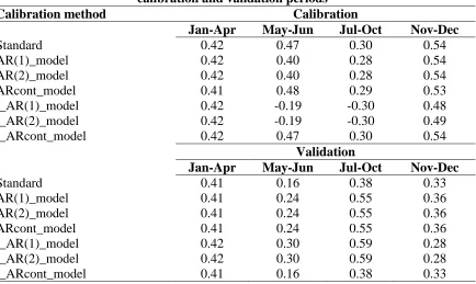
Table 4.7: NS values at different seasons for streamflow simulation during calibration and validation periods ... 66
Table 4.8: Effects of NS values at different seasons for streamflow simulation considering high sensitive and high and low sensitive parameters... 68
Table 4.9: Average annual evapotranspiration and streamflow using the model parameters at the maximum posterior density ... 68
Table 4.10: Efficiency of optimum values of model parameters in streamflow prediction during validation period ... 68
Table 4.11: Percentage of observed streamflow data covered by 95% prediction uncertainty due to parameter uncertainty during model calibration and validation periods ... 70
Table 4.12: Percentage of observed streamflow data covered by 95% prediction uncertainty during model calibration and validation periods ... 70
Table 5.1: Summary of the explicit methods used for SWAT model calibration... 107
Table 5.2: The prior ranges of parameters ... 110
Table 5.3: Comparison of mean (standard deviation) of SWAT model parameters ... 132
Table 5.4: Correlation between estimated model parameters ... 132
Table 5.5: Efficiency of SWAT model parameters obtained at the maximum posterior density ... 132
Table 5.6: Percentage of observed streamflow data covered by 95% prediction uncertainty... 134
Table 5.7: Quality of data covered by 95% prediction uncertainty ... 134
Table 5.8: Comparison of three calibration methods based on multiplicative input error model... 138
Table 6.1: The prior ranges of parameters ... 148
Table 6.2: Correlation between estimated SWAT model parameters ... 150
Table 6.3: Streamflow and precipitation characteristics of the watersheds for the period of 1981-2000 ... 167
Table 6.4: Comparison of results with seasonal input error model for two watersheds 168 Table 6.5: The prior ranges of parameters ... 171
Table 6.6: Optimum values of SWAT model parameters with 95% confidence limits for the Ruscom River watershed ... 174
xiii
Table 6.8: Efficiency of optimum parameter values for streamflow simulation in the Ruscom River watershed ... 175 Table 6.9: Percentage of observed streamflow data covered by 95% prediction
uncertainty in the Ruscom River watershed ... 177 Table 6.10: Reliability of streamflow prediction in the Ruscom River watershed ... 179 Table 6.11: Correlation of SWAT model parameters for the Canard River watershed .. 186 Table 6.12: Optimum values of SWAT model parameters with 95% confidence limits
for the Canard River watershed ... 186 Table 6.13: Efficiency of optimum parameter values for streamflow simulation in the
Canard River watershed ... 187 Table 6.14: Percentage of observed streamflow data covered by 95% prediction
xiv
LIST OF FIGURES
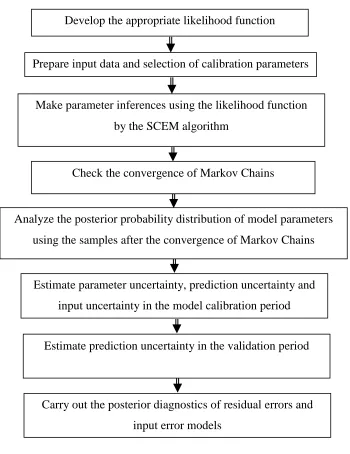
Figure 3.1: The flow chart for calibration of SWAT model under any uncertainty
framework ... 27 Figure 3.2: Movement of water simulated by SWAT at the HRU level for the study area
(Adapted from Neitsch et al., 2005)... 30 Figure 3.3: The computational framework of SWAT model calibration considering the
input error model... 34 Figure 4.1: Location of the Canard River watershed ... 51 Figure 4.2: Delineation of the Canard River watershed into sub-basins ... 52
Figure 4.3: Marginal posterior pdfs of model parameters in white noise and AR model
based calibration methods ... 56
Figure 4.4: Marginal posterior pdfs of model parameters in data transformation based
calibration methods ... 57
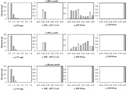
Figure 4.5: Marginal posterior pdf of AR model parameters in AR model based
calibration methods ... 58
Figure 4.6: Marginal posterior pdf of AR model parameters and transformation
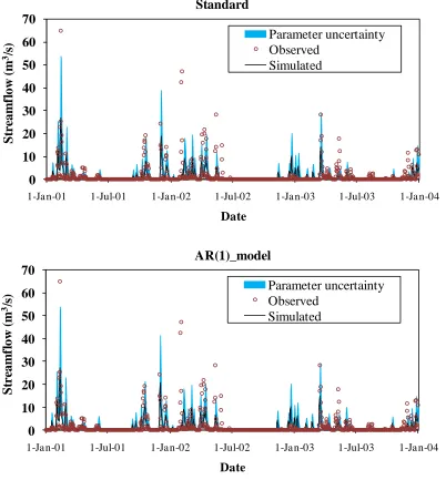
parameters in data transformation based calibration methods ... 59 Figure 4.7: Correlation between the estimated model parameters ... 62 Figure 4.8: Verification of parameter non-identifiability in the calibration process ... 64 Figure 4.9: Streamflow prediction uncertainty due to parameter uncertainty in calibration period in Standard and AR(1) model based calibration methods ... 72 Figure 4.10: Streamflow prediction uncertainty due to parameter uncertainty in
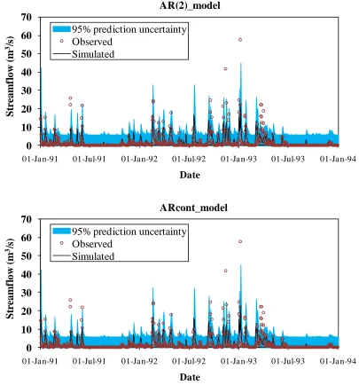
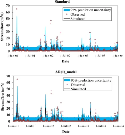
calibration period in AR(2) model and continuous AR model based calibration methods ... 73 Figure 4.11: Streamflow prediction uncertainty due to total uncertainty in calibration
period in Standard and AR(1) model based calibration methods ... 74 Figure 4.12: Streamflow prediction uncertainty due to total uncertainty in calibration
period in AR(2) model and continuous AR model based calibration methods ... 75 Figure 4.13: Streamflow prediction uncertainty due to parameter uncertainty in validation period for Standard and AR(1) model based calibration methods ... 77 Figure 4.14: Streamflow prediction uncertainty due to parameter uncertainty in validation period for AR(2) model and continuous AR model based calibration methods ... 78 Figure 4.15: Streamflow prediction uncertainty due to total uncertainty in validation
period for Standard and AR(1) model based calibration methods ... 79 Figure 4.16: Streamflow prediction uncertainty due to total uncertainty in validation
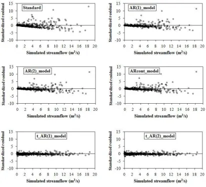
period in AR(2) model and continuous AR model based calibration methods ... 80 Figure 4.17: Test of homoscedasticity of standardized residuals ... 81 Figure 4.18: ACF and PACF plot of residuals with 95% limits in Standard calibration
method... 83 Figure 4.19: ACF plot of residuals with 95% limits in AR model based and data
transformation based calibration methods ... 85 Figure 4.20: Normality plot of standardized residuals in Standard and AR model based
calibration methods ... 87 Figure 4.21: Normality plot of standardized residuals in data transformation based
xv
Figure 4.22: Cumulative periodogram of residuals with 95% limits in Standard and AR
model based calibration methods ... 89
Figure 4.23: Cumulative periodogram of residuals with 95% limits in data transformation based calibration methods ... 90
Figure 5.1: Marginal posterior pdfs of SWAT model parameters in Standard, seasonal input error model and daily input error model based calibration methods ... 111
Figure 5.2: Box plots of marginal posterior probability distribution of seasonal input error model parameters ... 114
Figure 5.3: Deviation of estimated precipitation by seasonal input error model against the measured precipitation. ... 115
Figure 5.4: Marginal posterior probability distribution of daily input error model parameters. ... 115
Figure 5.5: Comparison of observed and estimated precipitation and observed and simulated streamflow in seasonal input error model and daily input error model based calibration methods. ... 116
Figure 5.6: Probability distribution function of DRMSE in different calibration methods. ... 117
Figure 5.7: Streamflow prediction uncertainty due to total uncertainty and parameter uncertainty in the calibration period. ... 119
Figure 5.8: Streamflow prediction uncertainty due to total uncertainty and parameter uncertainty in the validation period. ... 121
Figure 5.9: Predictive QQ plot in calibration and validation periods. ... 123
Figure 5.10: (a) QQ plot of standardized residuals and (b) ACF of residuals with 95% probability limits during calibration. ... 124
Figure 5.11: Test of homoscedasticity of standardized residuals during calibration. ... 126
Figure 5.12: Identification of precipitation events in the study area from February, 1992 to January, 1993. ... 128
Figure 5.13: Marginal posterior pdf of precipitation multipliers. ... 130
Figure 5.14: Marginal posterior pdf of SWAT model parameters. ... 131
Figure 5.15: Streamflow prediction using the parameter values at the maximum posterior density ... 133
Figure 5.16: QQ plot of standardized residuals in Standard and Storm_input_error methods. ... 136
Figure 5.17: ACF plot of residuals in Standard and Storm_input_error methods. ... 137
Figure 6.1: Location of the Ruscom River watershed ... 144
Figure 6.2: Delineation of the Ruscom River watershed into sub-basins ... 146
Figure 6.3: Marginal posterior pdfsof SWAT model parameters in Standard and seasonal input error model based calibration methods ... 149
Figure 6.4: Box plots of marginal posterior probability distribution of seasonal input error model parameters ... 152
Figure 6.5: Deviation of estimated precipitation by seasonal input error method against the measured precipitation. ... 153
Figure 6.6: Comparison of observed and estimated precipitation and observed and simulated streamflow in seasonal input error model based calibration method and Standard calibration method. ... 154
xvi
Figure 6.8: Streamflow prediction uncertainty due to total uncertainty and parameter
uncertainty in the calibration period. ... 158
Figure 6.9: Streamflow prediction uncertainty due to total uncertainty and parameter uncertainty in the validation period. ... 159
Figure 6.10: Predictive QQ plot in calibration and validation periods. ... 160
Figure 6.11: QQ plot of standardized residuals during calibration. ... 162
Figure 6.12: ACF plot of residuals with 95% probability limits during calibration. ... 163
Figure 6.13: Test of homoscedasticity of standardized residuals during calibration. ... 164
Figure 6.14: Location of the Canard River and Ruscom River watersheds... 166
Figure 6.15: Marginal posterior pdfsof SWAT model parameters for the Ruscom River watershed ... 173
Figure 6.16: Marginal posterior pdf of AR(1) model parameters for the Ruscom River watershed ... 174
Figure 6.17: Posterior pdfs of standard deviation of errors in AR(1) model based calibration method and DRMSE in seasonal input error model based calibration method in the Ruscom River watershed. ... 176
Figure 6.18: Predictive QQ plots in calibration and validation periods in the Ruscom River watershed. ... 178
Figure 6.19: QQ plot of standardized residuals in the Ruscom River watershed. ... 180
Figure 6.20: ACF of residuals with 95% probability limits in the Ruscom River watershed. ... 181
Figure 6.21: Test of homoscedasticity of standardized residuals in the Ruscom River watershed. ... 182
Figure 6.22: Cumulative periodogram of residuals with 95% limits in the Ruscom River watershed ... 183
Figure 6.23: Marginal posterior pdfsof SWAT model parameters for the Canard River watershed ... 185
Figure 6.24: Marginal posterior pdf of AR(1) model parameters for the Canard River watershed ... 187
Figure 6.25: Posterior pdfs of standard deviation of errors in AR(1) model based calibration method and DRMSE in seasonal input error model based calibration method in the Canard River watershed. ... 188
Figure 6.26: Predictive QQ plots in calibration and validation periods in the Canard River watershed. ... 191
Figure 6.27: QQ plot of standardized residuals in the Canard River watershed ... 192
Figure 6.28: ACF of residuals with 95% probability limits in the Canard River watershed ... 193
Figure 6.29: Test of homoscedasticity of standardized residuals in the Canard River watershed. ... 194
1 CHAPTER I
INTRODUCTION
1.1 General
The hydrological models are used for generating information on different
components of the hydrologic system. The model needs to be calibrated against the
observed data over a historical period of time before using the modeling results. During
the process of calibration, the model parameters are estimated such that the modeling
results are close to the observations of the real world system. There is uncertainty in the
results of any modeling that arises from different sources (Kay et al., 2009). The
uncertainties in the hydrological modeling are due to the uncertainty in model inputs,
parameters, structure and outputs (Thyer et al., 2009; Yang et al., 2008; Ajami et al.,
2007; Huard and Mailhot, 2006; Kavetski et al., 2006a; Vrugt, 2004). The uncertainty in
model inputs, such as precipitation, temperature, evapotranspiration etc., can result from
their measurement errors. The uncertainty in model parameters may arise from the
non-identifiable model parameters and non-uniqueness of non-identifiable model parameters. The
non-identifiable problem arises when model parameters are not identified as the
parameters that are required to be estimated through the calibration process. The problem
of non-uniqueness or equifinality arises when different sets of model parameters produce
similar observed responses for the hydrologic system. The uncertainty in model structure
is due to the simplification of the complex hydrological system and inadequate
representation of the system (Abbaspour, 2008). The uncertainty in model outputs is from
the measurement errors of the observed data. All sources of uncertainty can propagate
2
system (Ajami et al., 2008). Thus, proper quantification of uncertainty in model inputs,
parameters and predictions is vital for different water resources management problems,
such as watershed management, flood control and flood management, aquifer
management, reservoir management etc. Considering the importance of uncertainty
estimation, Pappenberger and Beven (2006) recommended to develop a 'Code of Practice'
for making the uncertainty analysis as an integral part of the hydrological modeling
process.
1.2 Uncertainty analysis in hydrological modeling
In the last two decades, many uncertainty analysis techniques were developed to
account for different sources of uncertainty explicitly or implicitly in the hydrological
modeling. The traditional uncertainty analysis techniques assume that all sources of
uncertainties in the hydrological modeling can be accounted for by the parameter
uncertainty. Some examples of these techniques are Sequential Uncertainty Fitting
(SUFI-2) (Abbaspour et al., 2007, 2004), Generalized Likelihood Uncertainty Estimation
(GLUE) (Beven and Binley, 1992), etc. In SUFI-2, the model parameters are calibrated
so that most of the observed data fall within the 95% prediction uncertainty bound
(Abbaspour et al., 2007). The GLUE methodology is an informal Bayesian approach
(Vrugt et al., 2009) and based on the concept of equifinality of model structure and/or
parameter sets in providing 'behavioral' fits to observational data (Zheng and Keller,
2007). The GLUE methodology has subjectivity in defining the likelihood function and
the behavioral criterion of the model (Blasone et al., 2008). For avoiding the subjectivity
in the likelihood function, some direct methods were introduced to account for different
3
in model inputs, structure and outputs are accounted for explicitly by introducing
appropriate error models to the calibration framework. The Bayesian Total Error Analysis
(BATEA) framework developed by Kavetski et al. (2006a) and the Bayesian framework
developed by Huard and Mailhot (2008) fall under the explicit methods. In BATEA
(Kavetski et al., 2006a), the input uncertainty is accounted for by assuming a
multiplicative error model, the structural uncertainty is represented by varying some
model parameters stochastically and the output uncertainty is accounted for by an
additive error model. In BATEA, the input and structural error parameters are treated as
latent variables to the hierarchical Bayesian modeling. However, Huard and Mailhot
(2008) represented different sources of errors by additive error models and the model
input and output time series were treated as latent variables to the Bayesian system. In the
Bayesian approach, the model parameters are considered as probabilistic variables and
the posterior probability density function of parameters are estimated by conditioning on
the observed data (Vrugt, 2004; Engeland and Gottschalk, 2002). The parameter
inferences are often made by the Markov Chain Monte Carlo (MCMC) methods for
estimating the posterior probability density function of model parameters. The posterior
probability density function is proportional to the product of the likelihood function and
the prior probability density function of parameters. The dimension of the posterior
probability distribution increases with the increase of number of variables needed to be
inferred and the numerical solution of posterior distribution becomes computationally
intensive. Hence, the high-dimensional problem of posterior probability distribution as
4
Kavetski et al. (2006a) and Huard and Mailhot (2008) are applied for the long calibration
period.
Ajami et al. (2007) introduced the Integrated Bayesian Uncertainty Estimator
(IBUNE) framework to account for model input, parameter and structural uncertainties.
They used the multiplicative error model to account for input uncertainty and the
multi-model combination technique to account for the structural uncertainty. Reichert and
Mieleitner (2009) corrected the bias in model input and structure explicitly by
introducing the stochastic, dependent model parameters. In this approach, the
time-dependent model parameter is considered as the multiplicative factor of, or additive term
to, the model input (Reichert and Mieleitner, 2009) and thus, it is conceptually similar to
the multiplicative error model of BATEA. Data assimilation techniques (Salaman and
Feyen, 2009; Moradkhani et al., 2005; Vrugt et al., 2005) are often used to account for
different sources of uncertainty in hydrological modeling. In the method, the state
variables are estimated at each time step of model simulation and thus, it has a
computational burden (Yang et al., 2007a).
In the indirect methods of uncertainty analysis, the errors in model inputs,
parameters, structure and outputs are lumped together and expressed implicitly as an
additive error model. Some examples of this category are the works of Schoups and
Vrugt (2010), Laloy et al. (2010), Schaefli et al. (2007), Yang et al. (2007a,b), Engeland
et al. (2005), Bates and Campbell (2001), Duan et al. (1988), Kuczera (1983), and
Sorooshian and Dracup (1980). The additive error model in the likelihood function aims
to make the residuals to be independent and normally distributed with zero mean and
5
non-constant variance (heteroscedastic). The autoregressive (AR) models are commonly
adopted in the implicit methods to account for the correlated errors of residuals (Laloy et
al., 2010; Vrugt et al., 2009; Schaefli et al., 2007; Yang et al., 2007a,b; Bates and
Campbell, 2001; Duan et al., 1988; Kuczera, 1983; Sorooshian and Dracup, 1980) and
the Box-Cox transformation (Box and Cox, 1964) of data is used to reduce the
heteroscedasticity and non-normality of the errors (McLeod et al., 1977; Box and Tiao,
1973).
The explicit methods of uncertainty analysis have some advantages over the
implicit methods. In the explicit methods, the effects of different sources of errors on the
uncertainty in model prediction can be quantified separately (Renard et al., 2010; Thyer
et al., 2009; Huard and Mailhot, 2008). However, the explicit methods are very
challenging when applied to the distributed hydrological modeling. A large number of
model parameters are used in a distributed hydrological model to describe the hydrologic
system and it becomes very difficult to identify the effects of the error models on
parameter estimation and model prediction (Abbaspour, 2008). In addition, the
computational burden is a constraint for using the explicit methods in uncertainty analysis
of the distributed hydrological modeling. Due to the challenges of the explicit methods,
the implicit methods are often used for quantifying uncertainty in the distributed
hydrological modeling.
1.3 Input uncertainty in distributed hydrological modeling
The uncertainty in precipitation data is the major source of input uncertainty in
any hydrological modeling. This type of uncertainty may result from the errors in
6
hydrological modeling (Huard and Mailhot, 2006). The precipitation measurement errors
may occur at a station due to the effects of wind and evaporation during its measurement
and/or instrument error (Salamon and Feyen, 2009). Even though the precipitation
measurement is exact, there might be differences between the gauge readings and the
model inputs due to the spatial scale difference (Huard and Mailhot, 2006). This
difference can be treated as the errors due to imperfect representation of precipitation.
Hwang (2005) identified the interpolation techniques of precipitation as a source of input
uncertainty in hydrological modeling. The uncertainty in model inputs propagates
through the calibration process and causes biasedness in parameter estimation. This
results in an increase in model prediction uncertainty. Therefore, the input uncertainty
needs to be taken into account during the model calibration process. In BATEA (Kavetski
et al., 2006a), the systematic measurement errors of precipitation data are corrected
during the calibration process directly by the rainfall multipliers, which are the latent
variables to the hierarchical Bayesian system. The temporal scale of the multipliers is
either daily or storm-event basis. Thus the dimension of the posterior probability
distribution is very high. The input uncertainty represented by the additive input error
model (Huard and Mailhot, 2008) has the dimensional problem as well, when the
resolution of temporal scale is finer than a month. The sequential data assimilation
techniques used to account for input uncertainty are also computationally intensive.
Due to the dimensional and computational constraints of the existing
multiplicative input error model, additive input error model and sequential data
assimilation method, input uncertainty is commonly corrected implicitly in aggregation
7
2009; Li et al., 2009; Yang et al., 2007a,b). Zhang et al. (2009) used the combined
method of Genetic Algorithms (GA) and Bayesian Model Averaging (BMA) for
calibration and uncertainty analysis of SWAT model. Li et al. (2009) used the Metropolis
algorithm based MCMC approach for uncertainty analysis of SWAT model. Yang et al.
(2007a,b) used the continuous time AR model to account for different sources of
uncertainty in SWAT model prediction.
The GLUE methodology (Beven and Binley, 1992) has often been used for
uncertainty analysis in the distributed hydrological modeling. Some examples are the
research of Younger et al. (2009), Yang et al. (2008), Blasone et al. (2008) and Arabi et
al. (2007). Younger et al. (2009) applied the GLUE methodology to study the effects of
spatial variability of rainfall on TOPMODEL (Beven et al., 1995). Yang et al. (2008)
applied GLUE methodology (Beven and Binley, 1992) for analyzing uncertainty of
SWAT model (Arnold et al., 1998). Blasone et al. (2008) used the GLUE methodology
for assessing all sources of uncertainty of MIKE-SHE model (Graham and Butts, 2006)
during multi-response and multi-site calibration. Arabi et al. (2007) used the GLUE
methodology for analyzing uncertainty of water quality estimates of SWAT model
(Arnold et al., 1998) for the best management practices. Salamon and Feyen (2009) used
the sequential data assimilation technique with the particle filter and assessed the
uncertainties in model parameter, precipitation and model prediction associated with
LISFLOOD model (De Roo et al., 2000).
The recent research direction in any hydrological modeling is to quantify the
effects of different sources of errors on model prediction. The effects of different sources
8
the explicit methods of uncertainty analysis. Hence, more studies are needed to reduce
the dimensional problem of posterior probability distribution so that the explicit methods
can be considered as a robust method of uncertainty analysis and can be practiced to
quantify uncertainty in the distributed hydrological modeling.
1.4 Objectives of the research
This dissertation addresses the existing limitations of the explicit methods of
uncertainty analysis and aims to develop a methodology under the Bayesian approach to
account for precipitation uncertainty explicitly in the calibration process of a distributed
hydrological model. The study is carried out with a widely-used distributed hydrological
model called Soil and Water Assessment Tool (SWAT) (Arnold et al., 1998). The
specific objectives of the dissertation are described as follows:
i) Quantifying the uncertainty in parameter estimation and model prediction by
the implicit methods of uncertainty analysis. The purpose of this objective is to identify
the merits and limitations of the implicit methods for the distributed hydrological models.
ii) Quantifying the parameter uncertainty and prediction uncertainty by
implementing the existing multiplicative input error models. This objective is carried out
to illustrate the need for development of a new method for the treatment of precipitation
uncertainty.
iii) Development of a new seasonal input error model to account for precipitation
uncertainty in the distributed hydrological modeling. The method is developed by
introducing the season-dependent parameters to the multiplicative input error model.
iv) Evaluation of the seasonal input error model by quantifying input uncertainty,
9
objective is to identify the robustness of the seasonal input error model in parameter
estimation and model prediction.
v) Application of the seasonal input error model to another watershed having
similar hydrologic and climatic conditions. The purpose of this objective is to investigate
the performance of the seasonal input error model for analyzing uncertainty of watershed
modeling.
1.5 Scope of the research
The dissertation carried out with the above objectives is expected to strengthen
the explicit methods of uncertainty analysis. The newly developed method is expected to
reduce the uncertainty in parameter estimation during calibration process and to reduce
the uncertainty in model prediction. The reduction of biasedness in parameter estimation
is important for parameter regionalization, while the improvement in model prediction is
useful for managing the extreme hydrological events. In addition, the newly developed
input error model expects to reduce the existing high-dimensional problem of the
multiplicative input error model and to identify the effects of input error model on
parameter estimation and model prediction in the distributed hydrological modeling.
1.6 Significance of the research
This research quantifies uncertainty in hydrological modeling arisen from inputs
and model parameters. The methodology of this research can be extended to the
uncertainty analysis of other water resources modeling studies, such as, hydraulic
modeling, water quality modeling and climate change impact studies. This research is
also significant for the studies related to transferring model parameters to the ungauged
10
explicitly in hydrological modeling. This research is probably the first attempt to extend
the explicit method of uncertainty analysis to distributed hydrological modeling. The
methodology developed in this dissertation will contribute to reducing dimensional
problem and computational cost of solving the posterior probability distributions.
Furthermore, this research develops a calibration method by representing the residual
errors with the second order autoregressive model. This is probably the first attempt to
implement the second order autoregressive model in the calibration process of any
hydrological modeling. Uncertainty estimation is usually communicated to the decision
makers for understanding the risk associated with uncertainty in modeling results.
Therefore, this research will contribute to managing water resources system.
1.7 Organization of the dissertation
The dissertation is organized into seven chapters. The literature related to the
existing uncertainty analysis methods is summarized in Chapter II. The methodology for
carrying out the objectives of the dissertation is presented in Chapter III. The first
objective is addressed in Chapter IV while the second, third and fourth objectives are
addressed in Chapter V. In Chapter IV, precipitation uncertainty is accounted for
implicitly along with other sources of uncertainties and the results are presented. In
Chapter V, precipitation uncertainty is taken care of explicitly and the seasonal input
error model is developed. The performance of the seasonal input error model is evaluated
in comparison with other existing multiplicative input error models. In Chapter VI, the
performance of the seasonal input error model for another watershed is evaluated. A
comparison is also made between the results obtained from the implicit method and
11
studies. Finally, in Chapter VII, the findings of the dissertation are presented in the
'conclusions' section and recommendations for future research are described in the 'future
12 CHAPTER II
LITERATURE REVIEW
2.1 Introduction
Most of the uncertainty analysis methods used in hydrological modeling are based
on the Bayesian approach. These methods can be classified into three major categories
based on how different sources of uncertainty are considered in the methods. Yang et al.
(2008) described these methods as: i) all uncertainties represented by parameter
uncertainty [Sequential Uncertainty Fitting (SUFI-2) (Abbaspour et al., 2007, 2004);
Generalized Likelihood Uncertainty Estimation (GLUE) (Beven and Binley, 1992)]; ii)
the input and model structural uncertainty considered implicitly by introducing an
additive error model [Schoups and Vrugt (2010); Laloy et al. (2010); Schaefli et al.
(2007); Yang et al. (2007a,b); Bates and Campbell (2001); Duan et al. (1988); Kuczera
(1983); Sorooshian and Dracup (1980)]; and iii) the input and/or model structural
uncertainty considered explicitly by using the stochastic time-dependent parameters
(Reichert and Mieleitner, 2009); additive input error model (Huard and Mailhot, 2008);
multiplicative input error model (Ajami et al., 2007, Kavetski et al., 2006a; Kuczera et
al., 2006); Sequential Data Assimilation (SDA) method (Moradkhani et al., 2005; Vrugt
et al., 2005. These methods of uncertainty analysis (UA) are described in this dissertation
as UA method-type 1, UA method-type 2 and UA method-type 3. This chapter briefly
discusses the Bayesian theory and hierarchical Bayesian modeling, the concepts,
application and limitations of three types of UA methods in hydrological modeling and
13
al., 1998). Moreover, the current state of knowledge in the field of 'uncertainty analysis'
and the research gaps are presented.
2.2 Bayesian theory
In the Bayesian approach, the model parameters are considered as probabilistic
variables having a joint posterior probability density function, which captures the
probabilistic beliefs about the parameters conditioned on the observed data (Vrugt, 2004).
According to the Bayesian theory, the posterior probability distribution of model
parameters, p( y)is expressed as follows (Gelman et al., 2004):
d y p p y p p d y p p y p y p ) ( ) ( ) ( ) ( ) ( ) ( ) , ( ) (
(2.1)
where p() is the prior distribution of parameters, p(y) is the sampling distribution
and
p()p(y)dis known as the normalizing constant. For a fixed y, this equation canbe written as:
) ( ) ( )
( y p p y
p (2.2)
The data y affects the posterior inference through the function p(y). When the data y
are given, p(y)can be considered as a function of which is known as the likelihood
function of given y (Gelman et al., 2004) and can be expresses as l( y). Thus eqn.
(2.2) can be written as:
) ( ) ( )
( y p l y
14 2.3 Hierarchical Bayesian modeling
According to Bayesian theory, for the parameters and given data, y, the
posterior probability distribution of is written as (eqn. (2.2))
) ( ) ( )
( y p y p
p (2.4)
where p()is the prior distribution of . If the prior distribution of depends on some
other parameters, ; according to hierarchical Bayesian modeling the posterior probability
distribution can be written as follows (Gelman et al., 2004):
) , ( ) , ( ) ,
( y p y p
p (2.5)
The prior p(,)can be replaced by a prior p(), and a prior of , p(), and
) ( ) ( ) , ( ) ,
( y p y p p
p (2.6)
The parameters are known as the hyperparameters in the hierarchical Bayesian
modeling. These variables are introduced in the system to modify the posterior
distribution of model parameters.
2.4 Methods of uncertainty analysis
UA method-type 1 assumes all sources of uncertainties in hydrological modeling
can be accounted for by parameter uncertainty. Hence, the methods aim to find the most
likely solutions of model parameters using a likelihood function and provide the
uncertainty in parameter estimation. Examples are SUFI-2 (Abbaspour et al., 2007, 2004)
and GLUE (Beven and Binley, 1992). In SUFI-2, the parameter uncertainty is described
by a multivariate uniform distribution in a parameter hypercube and the model
parameters are calibrated to bracket most of the measured data within the 95% prediction
15
95% prediction uncertainty (95PPU) calculated at the 2.5% and 97.5% levels of the
cumulative distribution of an output variable obtained through Latin Hypercube Sampling
(Abbaspour et al., 2007). Two indices, the P-factor and the R-factor, are used to quantify
the goodness of calibration/uncertainty performance. The P-factor is the percentage of
data bracketed by the 95PPU band (maximum value 100%), and the R-factor is the
average width of the band divided by the standard deviation of the corresponding
measured variable. In ideal condition when the uncertainty model is perfect, P-factor will
be 1 and the R-factor will be 0.
The GLUE approach is widely used for analyzing uncertainty in distributed
hydrological modeling. The GLUE approach is known as an informal Bayesian method
since it can be used with a statistically informal likelihood function (Vrugt et al., 2009).
In GLUE, the parameter sets are randomly sampled from the prior distribution of
parameters. All parameter sets meeting the predefined behavioral criterion are selected as
behavioral parameter sets and a 'likelihood weight' is given to each behavioral parameter
set. The prediction uncertainty is calculated by the percentiles of cumulative distribution
realized from the weighted behavioral sets. The major drawback of the GLUE approach
is its subjectivity of defining the likelihood function and the behavioral criterion (Blasone
et al., 2008).
UA method-type 2 considers the model residuals as a combination of errors due to
model inputs, parameters, model structure and outputs. In this approach, the residual
errors are represented by an additive error model to the model outputs. The residual
errors are described by a statistical model and the likelihood function is developed based
16
statistical error models are violated resulting in biasedness in parameter estimation. This
subsequently affects the parameter uncertainty and prediction uncertainty (Schoups and
Vrugt, 2010; Thyer et al., 2009). In classical calibration method, the model residuals are
described by the normal distribution with zero mean and constant variance and are
assumed to be uncorrelated. When the residuals are correlated (Schoups and Vrugt, 2010;
Laloy et al., 2010; Vrugt et al., 2009; Schaefli et al., 2007; Yang et al., 2007a,b; Bates
and Campbell, 2001; Duan et al., 1988; Kuczera, 1983; Sorooshian and Dracup, 1980),
the autoregressive (AR) models are used to remove the correlation of errors. When the
errors are heteroscedastic (Laloy et al., 2010; Vrugt et al., 2009; Schaefli et al., 2007;
Yang et al., 2007a,b; Bates and Campbell, 2001; Duan et al., 1988; Kuczera, 1983;
Sorooshian and Dracup, 1980) and non-normal (McLeod et al., 1977; Box and Tiao,
1973), the Box-Cox transformation (Box and Cox, 1964) of data is used. Recently
Schoups and Vrugt (2010) used an explicit statistical model to account for
heteroscedasticity and non-normality of residuals instead of using the Box-Cox
transformation of data. In their approach, the standard deviation of errors is modeled as a
linear function of simulated response to account for the heteroscedasticity and the error
distribution is described by considering the kurtosis and skewness of model residuals to
account for the non-normality of residuals (Schoups and Vrugt, 2010). Sometimes
Normal Quantile Transformation (NQT) is used to account for the non-normality of
residuals along with the AR model (Engeland et al., 2010).
Sorooshian and Dracup (1980) used the first order autoregressive [AR(1)] scheme
and the weighting approach with power transformation to reduce the correlation error and
17
autoregressive moving average (ARMA) model and the power transformation for the
similar problem. Duan et al. (1988) used the continuous time autoregressive error model
during the hydrologic model calibration for the autocorrelation error of data recorded at
unequal time interval. Bates and Campbell (2001) used the data transformation and the
higher order autoregressive model to remove the problems of non-constant variance and
autocorrelation of errors. They reported that the likelihood function based on data
transformation might not lead to independent, normally distributed residuals with zero
mean and constant variance. Schaefli et al (2007) used the AR(1) model to account for
the correlated errors and used a mixture of normal distribution error model with two
mixture components of high flow and low flow to account for the non-normality of
errors. Yang et al. (2007a) used the data transformation and continuous time
autoregressive error model to account for the heteroscedasticity and correlation of errors.
They used the seasonal variation of the statistical error model parameters such as
variance and characteristic correlation time to reduce the model structural uncertainty.
Yang et al. (2007b) used the t distribution to describe the residual errors to account for
the non-normality of residuals and continuous time autoregressive error model to account
for the correlation of errors. Laloy et al. (2010) used the data transformation and AR(1)
model to account for the non-constant variance and correlation of model residuals.
The major limitation of UA method-type 1 and UA method-type 2 is that the
effect of different sources of errors on hydrologic model prediction cannot be separated
using these methods. The effects of different sources of errors on model prediction
cannot be separated unless each source of errors is considered explicitly. In the UA
18
for and are represented by separate statistical error models (Renard et al., 2010; Huard
and Mailhot, 2008). Renard et al. (2010) used the BATEA framework (Kavestki et al.,
2006a) to identify the model input and structural errors. In BATEA, a multiplicative
Gaussian input error model which is independent for each storm is introduced and the
rainfall multipliers are considered as latent variables in the hierarchical Bayesian
modeling. The input error model of BATEA corrects the systematic error of rainfall
measurement on storm-event basis. Hence, the number of latent variables increases as the
length of calibration period increases and BATEA becomes computationally intensive.
BATEA has been used for quantifying prediction uncertainty in conceptual hydrological
models (Renard et al., 2010; Thyer et al., 2009; Kavetski et al., 2006b).
Huard and Mailhot (2008) developed a Bayesian uncertainty analysis framework
considering three errors of input, structural and output errors separately. There are two
common ways to relate errors and data, additively and multiplicatively. To allow the use
of Gaussian distributions, Huard and Mailhot (2008) applied additive error model. In this
method, the model input and output time series are the latent variables to the Bayesian
system and are inferred along with other model parameters. The approach is similar to the
approach implicitly used by Vrugt et al. (2005) in simultaneous optimization and data
assimilation (SODA) based on ensemble Kalman filters. The uncertainty framework is
developed for monthly time series data and the dimensional problem of posterior
probability distribution would arise if it is extended for daily time series.
Ajami et al. (2007) developed the Integrated Bayesian Uncertainty Estimator
(IBUNE) framework to account for input, output and structural uncertainties in
19
(Kavetski et al., 2006a) has been implemented in IBUNE by using the mean and variance
of the rainfall multipliers as latent variables in the Bayesian modeling. In IBUNE, the
model structural uncertainty is accounted for by the Bayesian model combination
approach. The IBUNE input error model reduces the high-dimensional problem of
BATEA input error model. The IBUNE multipliers are not storm dependent and can be
used in real-time forecasting to account for input error uncertainty (Ajami et al., 2009).
Even though the IBUNE input error model reduces the dimension of the posterior
distribution, Renard et al. (2009) reported some difficulties in implementing the IBUNE
input error model under the Bayesian framework. According to Renard at al. (2009), "the
likelihood and the posterior of IBUNE become random function of their arguments,
which violates the fundamental requirement for probability density functions." The
IBUNE input error model is also limited to be applicable for a relatively small variance
of rainfall multipliers (Ajami et al., 2009). Vrugt et al. (2008) applied the storm multiplier
concept (Kavetski et al., 2006a) for analyzing forcing data error explicitly in hydrologic
model calibration. While applying the storm multiplier concept, Vrugt et al. (2008)
assumed noninformative prior distribution of rainfall multipliers rather than informative
prior. Kavetski et al. (2006a) recommended using the informative prior to avoid the
ill-posedness in parameter inferences. Due to the high dimension of posterior distribution,
Kavetski et al. (2006a) suggested using the Newton-type optimization methods and
Hessian-based covariance analysis for solving the optimum parameter values. Vrugt et al.
(2008) developed the Differential Evolution Adaptive Metropolis (DREAM) algorithm
for solving the high-dimensional posterior probability distribution. The DREAM
20
(Vrugt et al., 2003), a global optimization algorithm. The DREAM algorithm maintains
detailed balance and ergodicity and is more applicable for complex, highly nonlinear and
multimodal target distributions (Vrugt et al., 2008). Vrugt et al. (2009) combined the
AR(1) model with the rainfall multiplier model to account for the structural, input and
parameter uncertainty.
Reichert and Mieleitner (2009) corrected the bias in hydrologic model or input
data explicitly by considering stochastic, time-dependent parameters rather than
considering bias in model outputs with AR error model. In this approach, the
time-dependent parameters are used to correct the rainfall time series which is similar to the
rainfall multipliers techniques (Kavetski et al., 2006a). This approach removes the
heteroscedasticity of the residuals by applying data transformation and is applicable to
nonlinear, dynamic models. Moradkhani et al. (2005) used the sequential data
assimilation approach for estimating model parameters and state variables using Bayesian
particle filters and observed improved uncertainty estimates of hydrological model
parameters. Sequential data assimilation is a process where the system state is recursively
estimated/corrected each time an observation becomes available (Moradkhani et al.,
2005). Vrugt et al. (2005) introduced a simultaneous parameter optimization and data
assimilation (SODA) method to assess the input, output, parameter and model structural
uncertainties in hydrologic modeling. They combined the strengths of the parameter
search efficiency and explorative capabilities of the Shuffled Complex Evolution
Metropolis (SCEM-UA) algorithm (Vrugt et al., 2003) with the power and computational
efficiency of the ensemble Kalman filter (Evensen, 1994). The main characteristic of
21
with state estimation. In SODA, different sources of errors are accounted for in terms of
state variables and the theoretical issues related to input errors are not focused (Huard and
Mailhot, 2006). The difficulty of SODA is that it involves state estimation and increases
the computational burden (Yang et al., 2007b).
2.5 Uncertainty analysis of SWAT model
SWAT is a commonly used distributed hydrological model for studying the
effects of land use change, climate change and management practices on water resources
system. Due to the extensive application of SWAT model, different techniques have been
developed for its uncertainty analysis. A suite of tools called SWAT calibration and
uncertainty programs (SWAT-CUP2) (Abbaspour, 2008) was developed for sensitivity
analysis, calibration, validation and uncertainty analysis of SWAT model. In
SWAT-CUP2, four uncertainty analyzing techniques are used for automated calibration and
uncertainty analysis of SWAT model. These are SUFI-2 (Abbaspour et al., 2004, 2007),
GLUE (Beven and Binley, 1992), Parameter Solution (Parasol) (Van Griensven and
Meixner, 2006) and Metropolis-Hastings based MCMC method. The method of
automated calibration and uncertainty analysis of highly parameterized SWAT model
has become convenient to apply due to the development of 'aggregate parameter concept'
(Yang et al., 2005). Some examples of applying the 'aggregate parameter concept' to
SWAT model are the research works of Li et al. (2010) and Yang et al. (2008; 2007a,b).
Setegn et al. (2010) used SUFI-2, Parasol and GLUE for estimating prediction
uncertainty of SWAT model for the Lake Tana Basin, Ethiopia. Li et al. (2009) used the
Bayesian MCMC approach for parameter estimation and uncertainty analysis of SWAT
22
small contributions of parameter uncertainty on model simulation uncertainty. Li et al.
(2010) also used the bootstrap method (Stine, 1985) for analyzing parameter uncertainty
of SWAT model in Yingluoxia watershed in northwest China. Ghaffari et al. (2010)
applied SWAT model for studying the impacts of land-use changes on hydrology of
Zanjanrood Basin, northwest Iran and used SUFI-2 for analyzing the uncertainty of
SWAT model prediction. Faramarzi et al. (2009) and Schuol et al. (2008) also used
SUFI-2 for analyzing uncertainty of blue and green water resources availability in Iran
and Africa, respectively using SWAT model. Xie and Zhang (2010) applied the
sequential data assimilation technique, the ensemble Kalman filter (EnKF) for combined
state-parameter estimation of SWAT model. Zhang et al. (2009) used the combined
method of Genetic Algorithms (GA) and Bayesian Model Averaging (BMA) for
calibration and uncertainty analysis of SWAT model. Yang et al. (2008) applied five
different uncertainty analysis techniques to the SWAT model; GLUE, Parasol, SUFI-2,
and a Bayesian framework implemented using MCMC and Importance Sampling (IS)
techniques. Yang et al. (2007a,b) used the continuous time AR models with Box-Cox
transformation of data for uncertainty analysis of SWAT model.
Since SWAT is a distributed model, the uncertainty in model prediction may arise
from the methods of distribution of rainfall inputs as well as from the spatial scale of
sub-watershed delineation. Cho et al. (2009) studied the effects of spatial distribution of
rainfall and the effects of sub-watershed delineation on the temporal and spatial
uncertainties of streamflow prediction and water quality results generated by SWAT
model. Kumar and Merwade (2009) studied the effects of sub-watershed delineation and
23
The literature shows that the physically based distributed model SWAT has been
extensively used for watershed management in different climatic and hydrologic
conditions. Different uncertainty analyzing methods are adopted for quantifying
parameter uncertainty and prediction uncertainty of SWAT model. Most of the methods
fall under category UA method-type 1. Explicit methods of analyzing uncertainty such as
BATEA (Kavetski et al., 2006a), IBUNE (Ajami et al., 2007), uncertainty framework of
Huard and Mailhot (2008) etc., have not yet been adopted for analyzing uncertainty of the
widely used SWAT model. The explicit methods assume specific error model for a
particular source of errors. For example, BATEA uses the multiplicative input error
model to account for rainfall uncertainty in hydrological modeling. The input error model
of BATEA assumes inputs as a random variable. Application of such input error models
for assessing uncertainty in SWAT model prediction is a challenging task due to the use
of a large number of variables to describe the hydrologic system (Abbaspour, 2008).
2.6 Current state of knowledge
To improve model parameter estimation and reducing parameter and prediction
uncertainties, many powerful numerical simulation and optimization tools, such as
Shuffled Complex Evolutionary Metropolis algorithm (SCEM-UA) (Vrugt et al., 2003),
Differential Evolution Adaptive Metropolis (DREAM) ((Vrugt et al., 2008), etc., have
been developed. These tools are being efficiently used for MCMC simulation and
uncertainty analysis. The recent research studies have been carried out for improving the
efficiency of optimization tools (Chu et al., 2010) and increasing the efficiency of
Markov Chain Monte Carlo (MCMC) sampler (Kuczera at el., 2010). Moreover, for
24
(2010) developed the 'model preemption' concept where a simulation model is terminated
early if the current model parameter set does not benefit the parameter searching scheme
by looking at the intermediate simulation model results.
2.7 Summary
Quantification of parameter and prediction uncertainty has been practiced for the
last three decades in hydrological modeling. Despite an extensive improvement in the
area of uncertainty in hydrological modeling, there are some research gaps. In distributed
hydrological modeling, the effects of different sources of errors on parameter estimation
and model prediction have not yet been quantified separately. Due to the difficulties in
implementing explicit methods, they are not commonly used for uncertainty analysis of
the distributed models. Moreover, the applicability of the multiplicative input error
models has not yet been explored for quantifying the input uncertainty in the distributed
hydrological modeling. The existing input error models have some dimensional and
computational problems when they are applied to the highly parameterized distributed
model for a long calibration period. The present study aims to develop a new uncertainty
analysis method suitable for a distributed hydrologic model. The SWAT model has been
selected as a tool for evaluating the performance of the developed methodology. The
study expects to reduce the existing research gaps of the uncertainty analysis by
introducing a season-dependent input error model for quantifying precipitation