Efficient sampling methods for truncated multivariate normal and student-t distributions subject to linear inequality

Efficient Sampling Methods for Truncated Multivariate

Normal and Student-t Distributions Subject to Linear

Inequality Constraints

Yifang Li

Department of Statistics, North Carolina State University

2311 Stinson Dr., Raleigh, NC, 27695

[email protected]

Sujit K. Ghosh

Department of Statistics, North Carolina State University

2311 Stinson Dr., Raleigh, NC, 27695

[email protected]

Abstract

Sampling from a truncated multivariate normal distribution subject to multiple linear

inequality constraints is a recurring problem in many areas in statistics and

economet-rics, such as the order restricted regressions, censored data models, and shape-restricted

nonparametric regressions. However, the sampling problem still appears non-trivial due

to the existence of the analytically intractable normalizing constant of the truncated

mul-tivariate normal distribution. In this paper, to start with, we develop an efficient mixed

rejection sampling method for the truncated univariate normal distribution, and

analyti-cally establish its superiority in terms of acceptance rates compared to some of the popular

existing methods. As the full conditional distributions of a truncated multivariate normal

distribution are truncated univariate normals, we employ the proposed superior univariate

sampling method and implement the Gibbs sampler for sampling from a truncated

mul-tivariate normal distribution with convex polytope restriction regions. We also generalize

are presented to illustrate the superior performance of our proposed Gibbs sampler in terms

of various criteria (e.g., accuracy, mixing and convergence rate).

Key words: truncated multivariate normal distribution, truncated multivariate Student-t

distribution, rejection sampling, Gibbs sampler, MCMC.

1

Introduction

The necessity of sampling from a truncated multivariate normal (TMVN) distribution subject

to multiple linear inequality constraints arises in many applied areas of research in statistics

and econometrics. Robert (1995) discusses several examples in order restricted (or isotonic)

re-gressions and censored data models. Several other applications are illustrated by Gelfand et al.

(1992), Liechty and Lu (2010) and Yu and Tian (2011), including the truncated multivariate

probit models in market research, and modeling co-skewness of the skew-normal distributions,

shape-restricted nonparametric regressions, and so on. The Bayesian normal linear regression

model subject to linear inequality restrictions is also a common application of the TMVN

dis-tributions, which is investigated in great details by Geweke (1996) and Rodrigues-Yam et al.

(2004).

Despite the wide range of applications mentioned above, an efficient method to generate

samples from a TMVN distribution is not so straightforward. One of the main barriers arises

from the complex normalizing constant involved in the probability density function (pdf) of

TMVN. Although the rejection sampling method can be used, it is hard to identify a well

working envelope function for the target distribution, and thus very low acceptance rates can

occur for some constrained regions. Moreover, even if we have an efficient sampling method

for the truncated univariate normal (TUVN) distribution, we cannot use direct sampling for

each element either. This is because of the fact that the marginal and the forward conditional

more efficient methods to avoid the evaluation of the normalizing constant, and also to utilize

the properties of the TMVN distribution itself.

The Gibbs sampler (Geman and Geman (1984) and Gelfand and Smith (1990)) has been

a populer technique in sampling from TMVN distributions. The Gibbs sampler is well suited

for the problem of sampling from TMVN distributions because all full conditional distributions

of a TMVN distribution are TUVN distributions. Majorities of the sampling methods for

generating samples from TMVN are based on the Gibbs sampler. An early survey is provided

by Hajivassiliou and Mcfadden (1990). Since the Gibbs sampler generates samples iteratively

from the full conditionals, the efficiency of this method is effectively determined by the efficiency

of sampling from the TUVN distributions. Breslaw (1994) suggests to use the uniform rejection

sampling method for the univariate full conditionals, which is recognized as not accurate or

efficient in many cases. Geweke (1991) and Robert (1995) both develop methods based on

various combinations of standard rejection sampling methods within the Gibbs sampler. These

methods are now widely used in statistics, and a few R packages are based on these methods.

Geweke (1991) also proposes a transformation on the restrictions of the TMVN distribution

before the Gibbs sampler is carried out. However, both of their methods for TUVN distributions

have low acceptance rates for certain types of interval restriction. Moreover, Geweke (1991)’s

Gibbs sampler suffers from slow convergence, and our empirical studies illustrate that this is

especially the case for unbounded regions. Rodrigues-Yam et al. (2004) propose another type of

transformation focusing on simplifying the covariance by uncorrelating the random vectors using

the square root of the covariance matrix instead of simplifying the restrictions, which somewhat

fix the poor mixing property of Geweke (1991)’s method.

The slice sampler (Neal (2003)) is also an appropriate technique for the sampling problem of

the TMVN distributions. Using this technique, Damien and Walker (2001) proposed to introduce

a single auxiliary variable and employ the univariate slice sampler to sample the TMVN random

samplers using multiple auxiliary variables and updating the entire random vector at a time.

This avoids the potential slow convergence of the Markov chain which can be caused by high

correlation between the components of the TMVN random vector. In their paper, they also

compare their method with the naive rejection method, and the one described in Neal (1997),

where a single auxiliary variable is used and the entire random vector is updated at a time,

and claim that their method is more efficient and accurate than the existing slice sampling

methods. However, their method only works for rectangular restriction regions, which limits

the applications of this method. Other methods can be seen in Yu and Tian (2011), where the

authors propose two sampling methods for TMVN distributions. One is a data augmentation

algorithm based on the EM algorithm, and the other one is a non-iterative inverse Bayes formulae

sampling procedure. These methods also update the random vector components together at

once.

In this paper, first we develop an efficient improved mixed rejection sampling method for

TUVN distributions that is shown to have uniformly larger acceptance rates than the existing

and widely used Geweke (1991)’s and Robert (1995)’s methods. Next we develop a Gibbs

sampler using our proposed TUVN sampling method to sample from the full conditionals of the

TMVN distributions subject to general linear inequality restrictions. Empirical results show

that our proposed Gibbs sampler has good mixing property and fast convergence regardless of

the type of the restriction regions. Moreover, as the multivariate Student-t distribution is a scale

mixture of the multivariate normal distribution, the sampling method of TMVN distributions

can be easily generalized to the truncated multivariate Student-t (TMVT) distributions. In

fact, any scale mixture of the multivariate normal distributions can be derived based on this

efficient sampling method. In this paper, we describe the algorithm for sampling from TMVT

distributions, and empirical study shows that this sampling method inherits the good mixing

property and fast convergence from the Gibbs sampler for TMVN.

distri-butions. The analytical acceptance rates of our mixed rejection sampling method for TUVN

distributions are calculated and compared to Geweke (1991)’s and Robert (1995)’s methods.

The results demonstrate that our method has uniformly larger analytical acceptance rates than

both of the existing methods. This sampling method is generalized to truncated multivariate

Student-t distribution in Section 3. In Section 4, we present the empirical acceptance rates

and display the histograms of the samples along with the true densities for TUVN distributions

overlayed. Further numerical examples with our Gibbs sampler for different TMVN and TMVT

distributions with various restriction regions are presented, to demonstrate the accuracy and

the fast convergence of the proposed method. In Section 5, we provide conclusions and further

discussions in this area. Proofs of the lemmas and other related additional results are included

in the appendices.

2

Efficient Truncated Normal Sampling Method

One of our main goals of this paper is to develop an efficient sampling method for the TMVN

distribution. A p-dimensional random variable W is said to have a truncated multivariate

(p-variate) normal distribution subject to linear inequality constraints, if its pdf satisfies

fW(w) =

exp−1

2(w−µ)

T_Σ−1

(w−µ)

R

c≤Rwe ≤dexp

−1

2(w−µ)TΣ

−1_{(w−µ) dw} I(c≤Rwe ≤d), (1)

where Σ is a non-negative definite matrix, I is the indicator function. The inequality notation

of c ≤ Rwe ≤ d means that the inequality holds element-wisely, i.e., c_i ≤ [Rw]e _i ≤ d_i for each

i = 1,2, . . . , p, with ci’s and di’s allowed to be −∞ and +∞, respectively. We denote this

TMVN distribution as

A good collection of statistical properties of TMVN distributions can be found in Horrace (2005).

In this paper, the proposed sampling method requiresRe to be am×pmatrix with rankm ≤p.

We state two key propositions of truncated multivariate normal distributions, which enable

the development of the proposed sampling methods. In the following propositions, we assume

that W has the distribution defined in (2).

Proposition 1. Let Y =AW, where A is a q×p matrix with rank q≤p. Then,

Y∼T Nq(Aµ,AΣAT;T), (3)

where T ={Aw:c≤Rwe ≤d}.

Proposition 2. PartitionX, µ and Σ as

X =



 

X1

X2





, µ=



 

µ₁

µ₂





, and Σ=



 

Σ11 Σ12

Σ21 Σ22



 .,

where X1 is a p1-dimensional random vector and X2 is a p2-dimensional random vector, and

p1+p2 =p. Then the conditional distribution of X1 given X2 =x2 is given by

X1|X2 =x2 ∼T Np1(µ1+Σ12Σ−221(x2−µ2),Σ11−Σ12Σ22−1Σ21;R1(x2)), (4)

where

R1(x2) = {x1 ∈Rp1 :a≤R(x1,x2)T ≤b}.

A similar result holds for the conditional distribution of X2 given X1 =x1.

It is worth mentioning that in both of (3) and (4), the restriction regions can not be explicitly

written in the form of c∗ ≤ Re∗x∗ ≤ d∗ for some Re∗, c∗ and d∗, however, the constraints are

distributed as in (2), we have

X=Σ−1/2(W−µ)∼T Np(0,I;R,a,b), (5)

where

R=RΣe 1/2, a=c−Reµ, and b=d−Reµ (6)

In (5), matrixΣ−1/2 denotes the inverse ofΣ1/2, which is the lower triangular Cholesky

decom-position of the covariance matrix Σ. Thus, without loss of generality, we focus on the sampling

method for the distribution in (5), which has a simpler form, instead of the general TMVN

random vector W.

It is well known that all full conditional distributions of TMVN are TUVN distributions.

This fact motivates us to use the Gibbs sampler (Geman and Geman (1984)) for generating

samples from the TMVN distribution, provided we have an efficient and accurate sampling

method to generate samples from the truncated univariate normal (TUVN) distribution.

The Gibbs sampler is well suited for the case where the joint distribution is non-standard

and is difficult to sample from, however, all of its full conditional distributions are some standard

distributions which are relatively easier to sample from. The Gibbs sampler iteratively samples

from the full conditional distribution producing an ergodic Markov chain which converges to the

2.1

Algorithms for Truncated Univariate Normal Distributions

In this section, we introduce our method for generating samples from a TUVN distribution. A

random variable W is said to follow a TUVN distribution, if its pdf satisfies

fW(w) =

1

σφ

w−µ

σ

Φ

d−µ

σ

−Φ

c−µ

σ

I(c≤w≤d) ∝ φ

w−µ

σ

I(c≤w≤d), (7)

where φ denotes the pdf of the standard normal distribution with mean 0 and variance 1, and

Φ denotes its cumulative distribution function (cdf). These notations will be used throughout

this paper. In the restriction, the bounds cand d are allowed to be −∞ and +∞, respectively.

We denote the distribution as

W ∼T N(µ, σ2;c, d). (8)

It easily follows that

X = W −µ

σ ∼T N(0,1;a, b), (9)

where a= (c−µ)/σ, andb = (d−µ)/σ, and the transformed random variable X has the pdf

given by

fX(x) =

φ(x)

Φ(b)−Φ(a)I(a≤x≤b). (10)

Suppose the sample generated from (9) is x, samples from W can be obtained by the

transfor-mationw=σx+µ. Therefore, without loss of generality, we will establish an efficient sampling

method for the TUVN random variable distributed as in (9).

Much of the research has been done on sampling methods for TUVN distributions. Gelfand

et al. (1992) propose to use the classical cdf inversion technique for sampling from fX(x). The

procedure is to sample u from U nif[Φ(a),Φ(b)], then the sample x can be obtained by setting

and its inverse Φ−1 _{for each draw. It is especially inefficient when the bounds are extreme as}

the numerical evaluations of Φ(a) and Φ(b) are only reasonably accurate when max(|a|,|b|)≤4,

otherwise Φ is essentially 0 or 1, which may cause computational issues for the bounds of the

uniform distribution. Furthermore, as u gets closer to 0 or 1, the computational time increases

and the precision gets poorer for the evaluation of Φ−1_(u).

Later work on seeking efficient sampling methods mainly focuses on avoiding the numerical

limitations of evaluating the cdf of normal distribution and its inverse. Geweke (1991) and

Robert (1995) develop the sampling methods based on accept-reject algorithm. The two

al-gorithms involve combinations of several rejection sampling methods. These mixed rejection

sampling methods are substantially more efficient than the cdf inversion technique in terms

of computational time and accuracy as no numerical integrations are required to sample

ran-dom variables. However, for a selected types of constraint intervals, they both suffer from low

acceptance rates.

In this section, we will develop a new mixed accept-reject algorithm, by combining four

standard rejection sampling methods. We seek the optimum acceptance rate among the four

re-jection sampling methods for every type of restriction boundaries, hence improve the acceptance

rate substantially compared to these two widely used sampling methods.

2.1.1 Basic Rejection Sampling Methods

The accept-reject algorithm is a common method for generating samples from a distribution.

More details can be seen in Chapter 2 of Robert and Casella (2004). This algorithm is stated

as a lemma below.

Lemma 1. To draw a sample from X ∼f(x), if for allx, there exists a constant M ≥1, and a

then it is sufficient to generate

x∼g and u∼U nif[0,1],

and take x as a sample from f(x), until u ≤ f(x)/(M g(x)). The resulting acceptance rate is

then 1/M, and this acceptance rate is maximized at

M =Mopt =

.

= sup

x:g(x)>0

f(x)

g(x).

Four basic rejection sampling methods are used in our mixed accept-reject algorithm for

gen-erating samples from TUVN distributions, which are defined by choosing the envelope function

g(x). The methods are the normal rejection sampling, the half-normal rejection sampling, the

uniform rejection sampling, and the translated-exponential rejection sampling. In this section,

we will describe each of the rejection sampling methods, and provide the optimized acceptance

rate for each method. From here on, a and b are finite numbers, unless mentioned differently.

Normal rejection sampling. Normal rejection sampling is a natural yet naive sampling method

for TUVN, in which we set the envelope functiong(x) =φ(x). Hence we draw a candidate

x from N(0,1), accept x as a sample of the TUVN if it is in the range of [a, b]. The

resulting acceptance rate is

Φ(b)−Φ(a). (11)

Here a and b are allowed to take the values as ±∞respectively.

Half-normal rejection sampling. When a ≥ 0, we can consider the half-normal rejection

is easy to show that the acceptance rate is

2(Φ(b)−Φ(a)). (12)

Here b is allowed to be +∞. Notice that this is more efficient than normal rejection

sampling when a ≥0.

Uniform rejection sampling. When the interval is bounded, uniform distribution can be

considered as the envelope distribution for sampling from TUVN distribution. We set

g(x) = 1/(b − a) as the pdf of U nif[a, b]. Since φ(x) is maximized at x = 0 if x is

unrestricted, the constant that maximizes the acceptance rate is given by

Mopt =

Φ(b)−Φ(a)

(b−a)φ{bI(b ≤0) +aI(a≥0)}.

Hence, the corresponding acceptance rate is

√

2π

b−a(Φ(b)−Φ(a)), if a≤0≤b; (13)

√

2π b−ae

a2

2 (Φ(b)−Φ(a)), if a≥0; (14)

√

2π b−ae

b2

2 (Φ(b)−Φ(a)), if b≤0.

Translated-exponential rejection sampling. The translated-exponential rejection sampling

method is initially considered for the type of the one-side restriction intervals with the

form of [a,∞] fora ≥0. The envelope density of this method is a a translated-exponential

distribution defined as

g(x) =λexp{−λ(x−a)}I(x≥a), (15)

a unit. As the lower bound a gets large, this translated-exponential distribution

resem-bles the TUVN distribution. We state the optimized acceptance rate of the one-sided

translated-exponential rejection sampling in the following lemma.

Lemma 2. The maximized acceptance rate of the one-sided translated-exponential rejection

sampling is

√

2πλ∗exp

−λ

∗2

2 +λ

∗

a

Φ(−a), (16)

where

λ∗ =. λ∗(a) = a+

√

a2_{+ 4}

2 . (17)

It is worth pointing out that, as a approaches ∞, the acceptance rate described in (16)

goes to 1, which illustrates that as a → ∞, the translated-exponential distribution starts

to resemble the TUVN distribution.

The translated-exponential rejection sampling method can also be used for two-sided

re-striction intervals as [a, b], provided that the upper bound b is relatively large. In the

two-sided translated-exponential rejection sampling, the candidatexis generated from the

translated-exponential distribution with pdf defined in (15), untilx≤b. Following a

sim-ilar procedure of maximizing the acceptance rate of the one-sided translated-exponential

distribution (as in Lemma 2), we get the maximized acceptance rate for the two-sided case

as

√

2π λ∗exp

λ∗a− 1

2λ

∗2

(Φ(b)−Φ(a)), (18)

where λ∗ is defined as in (17).

It is important to point out that choosing the value of λ as λ∗ does not increase the

computation time as stated in Geweke (1991). This is because for any given value of a, if

the translated-exponential rejection sampling is chosen for that region, λ∗ only needs to

2.1.2 Mixed Rejection Algorithm

We now compare the four basic rejection sampling methods described in Section 2.1.1 using a

case-by-case basis by maximizing the acceptance probability for all restriction intervals.

Ac-cording to the different natures and suitabilities of the basic rejection sampling methods, the

restriction intervals are divided into five cases. The five cases considered are:

• Case 1: one-sided region [a,∞);

• Case 2: two-sided region [a, b], where a <0< b;

• Case 3: two-sided region [a, b], where a ≥0;

• Case 4: one-sided region (−∞, b];

• Case 5: two-sided region [a, b], where b ≤0.

Note that the sampling method of TUVN with restriction region [−b,−a] can be directly derived

from the method for the restriction region [a, b], provided the method for the latter region is

given. To samplex∼T N(0,1;−b,−a), one can generatey ∼T N(0,1;a, b), and takex=−y. In

this sense, we call the regions [a, b] and [−b,−a] symmetric to each other. The above argument

also holds when a = −∞, or b = ∞. Hence, Case 4 is symmetric to Case 1, and Case 5 is

symmetric to Case 3. Therefore, we will focus on optimizing the sampling methods for the first

three cases, and the method for the last two cases can be obtained from their symmetric versions

respectively.

Generally speaking, it is well known that naively using only the normal rejection sampling

is impractical for TUVN sampling method. The normal rejection sampling may work well when

the mean 0 is contained in the region [a, b]. However, when a is several standard deviations

away to the right of 0, the normal rejection method sould be very inefficient. For the one-sided

of the half-normal rejection sampling method described in (12) is uniformly larger than the

acceptance rate of the normal rejection sampling as in (11), as long as half-normal rejection

sampling is suited for the type of regions. Hence, whenever half-normal rejection sampling can

be used, we favor it over the normal rejection sampling. The uniform rejection sampling method

generally produces satisfactory acceptance rate for narrow finite restriction regions. When the

whole region is above the mean 0, and for either one-sided region, or the two-sided region with

a relatively large upper bound, the translated-exponential rejection sampling is likely to be

preferred, as the shape mimics the TUVN distribution better and thus the method will result in

larger acceptance rates. We now explore the four basic rejection sampling methods and obtain

the best acceptance rates.

Case 1. As stated above, when a ≤ 0, the normal rejection sampling is the only available

method for the one-sided restriction regions. Thus it will be used when a ≤ 0. When

a > 0, both half-normal and translated-exponential rejection sampling methods can be

considered. Clearly, both of their acceptance rates are higher than the normal’s in (11).

Therefore, we only consider these two methods when a > 0. The comparison between

them is stated in the following lemma.

Lemma 3 (Half-norm vs. Translated-exponential). For the one-sided region with the form

[a,∞)witha≥0, there existsa0 >0, such that when 0< a < a0, the half-normal rejection

sampling method has larger acceptance rate, i.e., (12) is larger than (16). When a ≥ a0,

the translated-exponential rejection sampling method has larger acceptance rate, i.e., (16)

is larger than (12). In above, a0 is the solution of the equation

λ∗eλ

∗2 2 −1 =

r

2

π,

According to the result in Lemma 3, when 0< a < a0, we choose the half-normal rejection

sampling over the translated-exponential rejection sampling. When a is larger than a0,

the translated-exponential rejection sampling will be used.

Case 2. For this type of two-sided finite restriction regions, only the normal and the uniform

rejection sampling methods are suited. The results of comparing the acceptance rates of

the two methods are stated as follows.

Lemma 4 (Norm vs. Uniform). For the two-sided region with the form [a, b], where

a <0< b, whenb−a≤√2π, the uniform rejection sampling method has larger acceptance

rate, i.e., (13) is larger than (11); whenb−a >√2π, the normal rejection sampling method

has larger acceptance rate, i.e., (11) is larger than (13).

Thus, when b−a ≤ √2π, the uniform rejection sampling will be employed. Otherwise,

normal rejection sampling method will be used. This result complies with the fact that

the uniform rejection sampling performs better for shorter restriction regions.

Case 3. This type of two-sided regions require the most detail comparative analysis since all

four rejection sampling methods are available. However, as the acceptance rate of the

half-normal rejection sampling method described in (12) is uniformly larger than the

nor-mal rejection sampling method for any a and b, we do not consider the normal rejection

sampling for this case. We then focus on the comparisons among the other three methods

and the results are stated as follows.

Lemma 5(Half-normal vs. Uniform). For the two-sided regions with the form[a, b], where

a≥0, when

b < a+

r

π

2 exp

a2

2

.

=b1(a),

(12). Otherwise, the half-normal rejection sampling has larger acceptance rate, i.e., (12)

is larger than (14).

Lemma 6 (Uniform vs. Translated-exponential). For the two-sided regions with the form

[a, b], where a≥0, if

b≤a+ 2

a+√a2_{+ 4}exp

(

a2_−a√_a2 _{+ 4}

4 +

1 2

)

.

=b2(a), (19)

the uniform rejection sampling has larger acceptance rate, i.e., (14) is larger than (18).

Otherwise, the two-sided translated-exponential rejection sampling has larger acceptance

rate, ie.e, (18) is larger than (14).

Taking considerations of the results stated in Lemma 3, Lemma 5, and Lemma 6, for

Case 3, we first discriminate the situations according to the comparison between the

half-normal rejection sampling and the translated-exponential rejection sampling, as this

comparison only involves the value ofa. Hence, we first consider the case when 0≤a < a0.

Under this circumstance, when b ≤ b1(a), we will use the uniform rejection sampling

method; otherwise, we use the half-normal rejection sampling method. We then consider

the case when a≥a0. In this latter case, when b ≤b2(a), the uniform rejection sampling

is implemented for the TUVN sampling; otherwise the two-sided translated-exponential

sampling will be used.

Combining all the comparisons among the basic rejection sampling methods for all cases,

a globally optimal algorithm of our proposed mixed rejection sampling method is described as

follows:

Proposed Algorithm for TUVN:

(i) a≤0: use the normal rejection sampling,

(ii) 0< a < a0: use the half-normal rejection sampling,

(iii) a≥a0: use the one-sided translated-exponential.

Case 2 For the truncated interval 0∈[a, b]; if

(i) b > a+√2π: use the normal rejection sampling,

(ii) b≤a+√2π: use the uniform rejection sampling.

Case 3 For the truncated interval [a, b], a ≥0; if

(i) 0≤a < a0, and if

(a) b≤b1(a): use the uniform rejection sampling,

(b) b > b1(a): use the half-normal rejection sampling;

(ii) a≥a0, and if

(a) b≤b2(a): use the uniform rejection sampling,

(b) b > b2(a): use the two-sided translated-exponential rejection sampling.

Case 4 For the truncated interval (−∞, b]: use the symmetric algorithm to Case 1.

Case 5 For the truncated interval [a, b], b≤0: use the symmetric algorithm to Case 3.

2.1.3 Comparisons of Analytical Acceptance Rates

Our numerical studies show that generally, Robert (1995)’s outperforms Geweke (1991)’s for

Case 1 and Case 3, while the dominance reverses for Case 2, in terms of acceptance rates. As

a result, it is of interest to compare our proposed algorithm with that of Robert (1995)’s for

Cases 1 and 3, and with that of Geweke (1991)’s for Case 2. The analytical acceptance rates

Table 1: Analytical Acceptance Rates for Case 1: [a,∞)

a New Geweke Robert a New Geweke Robert

-2 0.977 0.977 0.977 0.2 0.841 0.417 0.790

-1 0.841 0.841 0.841 0.45 0.822 0.326 0.822

-0.5 0.691 0.691 0.691 1 0.876 0.656 0.876

0 1.000 0.500 0.760 5 0.983 0.964 0.983

Table 2: Analytical Acceptance Rates for Case 2: 0∈[a, b]

New Geweke Robert New Geweke Robert

b a=−2 a=−1

.5 0.670 0.669 0.670 0.890 0.890 0.890

1 0.819 0.819 0.684 0.856 0.856 0.856

2 0.954 0.954 0.598 0.819 0.819 0.684

b a=−0.5 a=−0.1

2 0.670 0.669 0.670 0.617 0.517 0.617

mixed rejection sampling method uniformly outperforms both of the two methods for all types

of regions.

These tables clearly show the sub-optimal performance in acceptance rates of the two widely

used existing methods, since none of them were created by maximizing the acceptance rates. In

Geweke (1991)’s algorithm, there are 4 constants serving as critical cut-off values of deciding

the separations of the utility of the basic rejection sampling methods, which are claimed to find

via computational empirical experiments only. However, theoretical analysis shows that this

may cause very low acceptance rates, such as in Case 1 when a= 0.45, which is approximately

the constant Geweke (1991) uses to divide the use of the normal and the translated-exponential

Table 3: Analytical Acceptance Rates for Case 3: [a, b], a≥0

New Geweke Robert New Geweke Robert New Geweke Robert

b a= 0 b a = 1 b a= 2

2 0.955 0.955 0.726 3 0.869 0.650 0.869 4 0.932 0.842 0.932

1 0.856 0.856 0.856 2 0.751 0.562 0.751 3 0.878 0.793 0.878

0.5 0.960 0.960 0.960 1.5 0.759 0.759 0.759 2.5 0.679 0.613 0.679

rejection sampling methods. The acceptance rate is as low as 0.326, which leads to a highly

in-efficient sampling method, especially when used within a Gibbs sampler. As for Robert (1995)’s

method, the half-normal rejection sampling method is not considered. Hence, the algorithm

does not take advantage of the similar nature of the half-normal distributions to the TUVN

dis-tribution when the lower bound is close to 0 for one-sided regions over the translated-exponential

distribution, or for loose bounded regions over the uniform distribution. For an example of the

low acceptance rate caused by Robert (1995)’s method, consider Case 1, when a = 0.2, and

Case 3, when a= 0 andb = 2.

Notice that in Table 1, whena = 0, our acceptance rate is exactly 1, becauseT N(0,1; 0,∞)

is exactly the half-normal distribution. On the contrary, for this case, Robert (1995)’s uses the

translated-exponential rejection sampling, and Geweke (1991) uses the naive normal rejection

sampling, which are inefficient compared to our proposed method. In Table 2 for Case 2, when

a+√2π = 0.5066 with a = 2, which is very close to the value of b = 0.5, hence the uniform

rejection sampling method is used and results in a slightly larger acceptance rate than Geweke

(1991)’s. Since in this case, Robert (1995)’s also utilizes the uniform rejection sampling, the

acceptance rate is exactly the same as ours. Also in Table 2, when a=−0.1 anda=−0.5, the

lower bound to use the normal rejection sampling is b = 2.01 and b = 2.4 respectively, hence

in both of the cases when b = 2, the uniform rejection sampling is used, which again results in

a larger acceptance rate than that of Geweke (1991)’s method which uses the normal rejection

sampling method. Moreover, Table 2 gives a clear illustration of the fact that the uniform

rejection sampling only performs well for shorter restriction intervals, as for Case 2, which is the

only sampling method that is used by Robert (1995). It can be seen that as the interval becomes

wider, the acceptance rate decreases significantly for the Robert (1995) method, yielding a low

acceptance rate of only 0.598 when a=−2 and b= 2, compared to our normal rejection which

has an acceptance rate of 0.954 in this case. Finally, consider the Case 3 shown in Table 3. In

method and that of Geweke (1991) method, the empirical methods used in fact can be different.

As in our method, the lower bound of using the half-normal rejection sampling is b = 1.253,

while in Geweke (1991)’s, that value is 1.249, which is very close to our cut-off value, hence

it is hard to make a difference between the two methods. Other than this value of a, Geweke

(1991)’s method yields much smaller acceptance rates. Furthermore, Geweke (1991)’s method

requires much more complicated computation involving two constants obtained empirically, and

the evaluations of the ratio of φ(a) to φ(b). Moreover, in the case of a = 0 and b = 2, our

method uses the half-normal rejection sampling, while Robert (1995)’s method uses the uniform

rejection sampling, which produces smaller acceptance rate.

Therefore, in any case of the restriction regions, our newly proposed method outperforms

both of the widely used existing methods with uniformly larger acceptance rates. This increases

the efficiency of sampling from the TUVN distributions, which serves as the building blocks for

the sampling method from the TMVN distributions within the Gibbs sampler. Moreover, as

our method does not involve much complicated computations, the running time of our sampling

program is similar to that of the other existing methods. We illustrate the empirical performance

of the proposed method in Section 4.

2.2

Algorithm for Truncated Multivariate Normal Distributions

Now that we have an efficient sampling method for TUVN distributions, we focus on the

sam-pling method from the TMVN distribution, which is the central interest of this paper. Although

naively applying the multivariate normal rejection method can be used, it is well known that

such a method would be highly impractical and inefficient. Direct rejection sampling methods

are also difficult to construct as it is hard to find an all purpose envelope function for TMVN

distributions. Methods for sampling from TMVN distributions also need to cope with the fact

many researchers have chosen the Gibbs sampler to sample from TMVN. In this paper, we will

use this technique and focus on developing an efficient Gibbs sampler for generating samples

from TMVN distributions.

To simplify the procedure of the Gibbs sampler, usually some transformations are done

before the Gibbs sampler is implemented. For any general TMVN distributed random vector

W ∼T Np(µ,Σ;Re,c,d) as in (2), Geweke (1991) proposes to use the transformation as

Z =R(We −µ). (20)

The motivation behind (20) is that the resulting restrictions of the random vector Z becomes

α≤Z≤β,

where α = a−Reµ and β = b −Reµ, hence the restrictions are explicitly defined for every

component without any linear summation involved. Although this transformation simplifies the

restrictions, according to Proposition 1, the distribution of Z is T Np(0,RΣe ReT;I,α,β), hence

the covariance matrix is not an identity matrix. By Proposition 2, the resulting full conditional

distributions required within the Gibbs sampler are also not truncated standard univariate

normal. As the sampling method is defined forT N(0,1;a, b) only, in each of the Gibbs updating

step, two transformations are required, one of which is to transform the nonstandard TUVN to

the standard TUVN, and another one is to transform the generated sample back to the original

full conditional distribution for later updating steps, and in each of the step, one matrix inversion

is needed. This causes inefficiency in Geweke (1991)’s sampling method for TMVN especially

when a large number of samples are of interest from a high dimensional TMVN distribution.

The nonidentity covariance matrix is also a source for the poor mixing in the Gibbs sampler.

and invertible, which limits the application of the method.

In this paper, as argued at the beginning of this section, we introduce the transformation

described in (5) as

X=Σ−1/2(W−µ),

The distribution of the obtained random vector is denoted as X ∼ T Np(0,I;R,a,b) in (9),

where Re and R are both m ×p matrices. This transformation focuses on transforming the

mean and the variance of the multivariate normal distribution, instead of the constraints of the

TMVN distribution. As a result, we do not require Re to be a square matrix, and hence we

allow that m ≤ p and require that the rows are linearly independent. The motivation of the

transformation (5) is that it greatly simplifies the pdf of W given in (1), as the transformed

random vector X has a truncated standard multivariate normal distribution with mean 0, and

covariance matrix I. By Proposition 2, the resulting full univariate conditional distribution is

xi|x−i ∼T N(0,1;a∗i(x−i), b∗i(x−i)), i= 1, . . . , p, (21)

where x−i = (x1, . . . , xi−1, xi+1, . . . , xp), and a∗i(x−i) and b∗i(x−i) are determined suitably such

that a ≤ Rx ≤ b. The full conditional distribution described in (21) shows the advantage of

making such a transformation, that in each updating step of the Gibbs sampler, we will deal

with a truncated standard univariate normal distribution. This procedure improves the poor

mixing of the Gibbs sampler proposed by Geweke (1991), especially for wider restriction regions.

Without loss of generality, we develop the sampling method for the random vectorX. To obtain

the samples for the original TMVN vector W, we simply use the following transformation

w=Σ1/2x+µ

trans-formations, and one matrix inversion on the Cholesky decomposition of the covariance matrix.

We next explain how to evaluate the lower and the upper boundsa∗_i andb∗_i in every updating

step. Let Ri denote the ith column of R, R−i denote the m×(p−1) matrix by removing the

ith column of R. Hence, the restrictions a≤Rx≤d is equivalent to

a−R−ix−i ≤Rixi ≤b−R−ix−i,

which is equivalent to the following coordinate-wise inequalities

aj−rj,−ix−i ≤rjixi ≤bj−rj,−ix−i, (22)

for all j = 1, . . . , m,, where rj,−i denotes thejth row of the matrix R−i, andrji denotes the jth

entry of the vector Ri. Depending on the sign of rji, we have three different scenarios:

When rji >0. For all j’s such that rji>0, (22) is equivalent to

aj −rj,−ix−i

rji

≤xi ≤

bj −rj,−ix−i

rji

.

Hence we define

l+_i = max

{j:rji>0}

aj −rj,−ix−i

rji

and u+_i = min

{j:rji>0}

bj−rj,−ix−i

rji

.

When rji <0. For all j’s such that rji<0, (22) is equivalent to

bj −rj,−ix−i

rji

≤xi ≤

aj −rj,−ix−i

rji

Hence we define

l−_i = max

j:rji<0

bj−rj,−ix−i

rji

and u−_i = min

j:rji<0

aj−rj,−ix−i

rji

.

When rji = 0. There is no restriction on xi for this j.

Combining all three scenarios discussed above, we have

a∗_i = max{l+_i , l−_i } and b∗_i = max{u+_i , u−_i }.

If a∗_i ≤b∗_i, these bounds can be used for sampling from the full conditional distribution in each

step of the Gibbs sampler. In fact, the region defined by{x:a≤Rx≤b}is a convex polytope.

Hence as long as the starting value is within the region, our method remains feasible in every

updating step. Therefore, in the ith step of the tth pass in the Gibbs sampler, we sample

x_i(t)|x(₁t), . . . , x_i(t₋)₁, x(_i+1t−1), . . . , x(_pt−1) ∼T N(0,1;a_i∗(t), b∗_i(t)), (23)

where a∗_i(t) = a_i∗(x(₁t), . . . , x_i(₋t)₁, x_i(₊₁t−1), . . . , x(pt−1)), and b

∗(t)

i = b

∗

i(x

(t)

1 , . . . , x

(t)

i−1, x (t−1)

i+1 , . . . , x

(t−1)

p ),

for i= 1, . . . , p.

Empirical results in Section 4 demonstrate that the proposed Gibbs sampler has very good

mixing property and converges very fast to the true joint truncated multivariate normal

distri-bution.

3

Efficient Truncated Student-T Sampling Method

The sampling method for TMVN distributions can be easily generalized to a method for sampling

from truncated multivariate Student-t (TMVT) distributions, as a TMVT can be obtained as

by its degree of freedom. In this section, we describe the algorithm of sampling from TMVT

distributions based on the efficient sampling method for TMVN distributions.

A random vector Y following a truncated multivariate (p-variate) Student-t distribution

with degree of freedom ν subject to linear inequality constraints c≤Rye ≤d is denoted as

Y ∼T Tp(µ,Σ, ν;Re,c,d). (24)

Following the property of a multivariate Student-t distribution, a similar transformation as in

(5) can be done such that

T=Σ−1/2(Y−µ)∼T Tp(0,I, ν;R,a,b), (25)

whereΣ−1/2,R,e a, andbare defined as in (6). Therefore, without loss of generality, we develop

the sampling algorithm for T. To obtain a sample y of the distribution given in (24) from a

sample t of that in (25), we only require a simple transformation as

y=Σ1/2t+µ.

We let

T∗ ∼Tp(0,I, ν)

denote an untrucatedp-variate Student-t distributed random variable with degree of freedom ν,

then by definition,

T∗ = X

∗

p

U/ν,

whereX∗ ∼Np(0,I) is a standardp-variate normal distributed random variable, andU ∼χ2(ν)

for a given sample ufrom the distribution of U, the linear constraints of Tcan be expressed by

a≤RT = _pRX

u/ν ≤b,

which implies that

apu/ν ≤RX≤bpu/ν.

These facts indicate that a Gibbs sampler can be used to sample from TMVT distributions

based on the existing TMVN sampling method.

The algorithm of the Gibbs sampler to obtain a sampletfrom the distribution given in (25)

is described as follows:

1. Sample u∼χ2_(ν).

2. Sample x∼T Np(0,I;R,a

p

u/ν,bpu/ν).

3. Set t= √x

u/ν.

In the second step, our proposed Gibbs sampler for TMVN sampling will be implemented.

As the efficiency and accuracy of the TMVT distributions are highly influenced by that of the

TMVN distributions, simulation studies given in Section 4 illustrate that this Gibbs sampler

inherits the good mixing property and fast convergence from the sampling method for TMVN

distributions.

4

Simulation Studies

In this section, we present several numerical illustrations to compare the performance of the

proposed sampler for TUVN, TMVN, and TMNT distributions with that of the other popular

Table 4: Simulated Acceptance Rates for Case 1: [a,∞)

a New Geweke Robert a New Geweke Robert

-2 0.977 0.977 0.977 0.2 0.840 0.421 0.790

-1 0.840 0.840 0.840 0.45 0.823 0.324 0.823

-0.5 0.695 0.695 0.695 1 0.880 0.656 0.880

0 1.000 0.495 0.763 5 0.984 0.969 0.984

Table 5: Simulated Acceptance Rates for Case 2: 0∈[a, b], a <0< b

New Geweke Robert New Geweke Robert

b a=−2 a=−1

.5 0.672 0.660 0.672 0.897 0.897 0.897

1 0.819 0.819 0.687 0.860 0.860 0.860

2 0.954 0.954 0.606 0.819 0.819 0.690

b a=−0.5 a=−0.1

2 0.680 0.673 0.680 0.624 0.515 0.624

4.1

Sampling from TUVN

In this sub-section, we present the empirical results for our proposed mixed rejection sampling

algorithm for TUVN distributions.

Tables 4 to 6 show the empirical acceptance rates along with the theoretical analytical

ac-ceptance rates given in Table 1 to 3. For each of the restriction intervals, 10,000 samples are

generated using three methods: our newly proposed method, Geweke (1991)’s, and Robert

(1995)’s. For each method, the empirical acceptance rates are computed as 10,000/Ntry, where

Ntry denotes the total number of trials until 10,000 samples are accepted. Similarly, the

accep-tance rates are calculated for Cases 1 to 3 ony, as Case 4 and Case 5 are symmetric to Case 1

and Case 3 respectively.

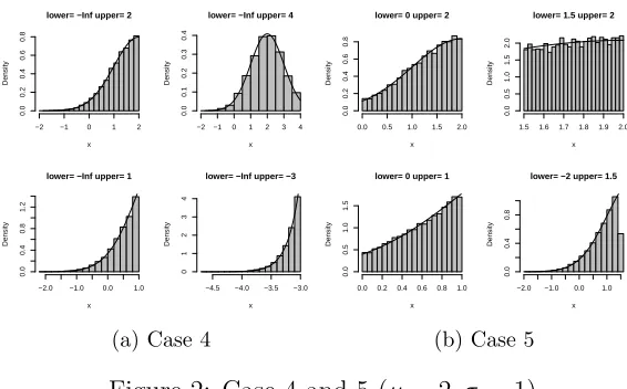
Figures 1 and 2 display the histograms of the samples obtained by our algorithm with the

exact density curves overlayed. In these examples, a T N(µ, σ2;c, d) with parameters µ = 2

and σ = 1 are used. The bounds are provided in the captions of the figures. The histograms

Table 6: Simulated Acceptance Rates for Case 3: [a, b], a≥0

New Geweke Robert New Geweke Robert New Geweke Robert

b a= 0 b a = 1 b a= 2

2 0.954 0.954 0.728 3 0.872 0.652 0.872 4 0.937 0.843 0.937

1 0.861 0.861 0.861 2 0.756 0.562 0.756 3 0.882 0.793 0.882

0.5 0.964 0.964 0.964 1.5 0.766 0.766 0.766 2.5 0.684 0.616 0.684

0.1 0.999 0.999 0.999 1.1 0.954 0.954 0.954 2.1 0.911 0.911 0.911

of the density of the TUVN. It is worth noticing that the figures displayed in Figure 2 for Case

4 and 5 and in Figure 1 for Cases 1 and 3 are symmetrical to the line x=µ, respectively, which

further re-establishes the fact that we only require symmetric algorithms for Cases 4 and 5. In

addition to depicting histograms, we also carried out statistical tests of goodness of fit (such as

Anderson-Darling test, Kolmogorov-Smirnov test, etc.), all of which further confirms the correct

generating mechanism of the proposed method.

lower= 2 upper= Inf

x

Density

2 3 4 5 6

0.0

0.2

0.4

0.6

0.8

lower= 0 upper= Inf

x

Density

0 1 2 3 4 5 6

0.0

0.1

0.2

0.3

0.4

lower= 3 upper= Inf

x

Density

3.0 4.0 5.0 6.0

0.0

0.4

0.8

1.2

lower= 7 upper= Inf

x

Density

7.0 7.5 8.0 8.5

0

1

2

3

4

(a) Case 1

lower= 0 upper= 2.5

x

Density

0.0 0.5 1.0 1.5 2.0 2.5

0.0

0.2

0.4

0.6

lower= 1 upper= 3

x

Density

1.0 1.5 2.0 2.5 3.0

0.0

0.2

0.4

0.6

lower= 1 upper= 4

x

Density

1.0 1.5 2.0 2.5 3.0 3.5 4.0

0.0

0.2

0.4

lower= 1.5 upper= 4

x

Density

1.5 2.0 2.5 3.0 3.5 4.0

0.0

0.2

0.4

0.6

(b) Case 2

lower= 2 upper= 4

x

Density

2.0 2.5 3.0 3.5 4.0

0.0

0.2

0.4

0.6

0.8

lower= 2 upper= 2.5

x

Density

2.0 2.1 2.2 2.3 2.4 2.5

0.0

0.5

1.0

1.5

2.0

lower= 3 upper= 4

x

Density

3.0 3.2 3.4 3.6 3.8 4.0

0.0

0.5

1.0

1.5

lower= 2.5 upper= 6

x

Density

2.5 3.5 4.5 5.5

0.0

0.4

0.8

(c) Case 3

Figure 1: Case 1, 2 and 3 (µ= 2, σ= 1)

4.2

Sampling from TMVN

In this sub-section, we illustrate our sampling method for several examples to explore how well

lower= −Inf upper= 2

x

Density

−2 −1 0 1 2

0.0

0.2

0.4

0.6

0.8

lower= −Inf upper= 4

x

Density

−2−1 0 1 2 3 4

0.0

0.1

0.2

0.3

0.4

lower= −Inf upper= 1

x

Density

−2.0 −1.0 0.0 1.0

0.0

0.4

0.8

1.2

lower= −Inf upper= −3

x

Density

−4.5 −4.0 −3.5 −3.0

0

1

2

3

4

(a) Case 4

lower= 0 upper= 2

x

Density

0.0 0.5 1.0 1.5 2.0

0.0

0.2

0.4

0.6

0.8

lower= 1.5 upper= 2

x

Density

1.5 1.6 1.7 1.8 1.9 2.0

0.0

0.5

1.0

1.5

2.0

lower= 0 upper= 1

x

Density

0.0 0.2 0.4 0.6 0.8 1.0

0.0

0.5

1.0

1.5

lower= −2 upper= 1.5

x

Density

−2.0 −1.0 0.0 1.0

0.0

0.4

0.8

(b) Case 5

Figure 2: Case 4 and 5 (µ= 2, σ = 1)

Example 1. In this example, we employ our method to truncated bivariate normal (TBVN)

distributions. We choose these TBVN distributions only for the sake of conveniently displaying

the accuracy of our sampling method on a contour plot of the distribution. This is difficult for

higher dimensional TMVN distributions due to the property that the marginal distributions are

not TMVN and have very complex pdf’s.

In this example, our method is implemented for a random vector X = (X1, X2)T which

is a bivariate normal distribution with µ = (0,0)T, V ar(X1) = 10, V ar(X2) = 0.1, and the

correlation matrix V=    1 ρ ρ 1   ,

truncated by the linear constraints given as

e R=    1 1

1 −1



We investigate 6 different restriction regions. We define



 

 

σ1 =

p

V ar(X1+X2) =

√

10.1 + 2ρ

σ2 =

p

V ar(X1−X2) =

√

10.1−2ρ

and sd=



 

σ1

σ2



 .

In the first 3 cases, the restriction regions are bounded in which X is truncated by ±1.5sd,

±0.15sd, and ±0.05sd, respectively. The fourth and the fifth restriction regions are one-sided

open regions, with the lower bounds set to be −0.15sd and 0.15sd, respectively, and the upper

bounds both set to be +∞. The final one is an extreme case where the lower and the upper

bounds are set to be ±∞ respectively, hence it is in fact an ordinary bivariate normal

distri-bution. For each of the restriction regions, we also test a moderate correlation between X1 and

X2 with ρ= 0.5, and a very high correlation with ρ= 0.98. The initial values for the fifth case

is (1,0)T, while those of all the others are (0,0)T.

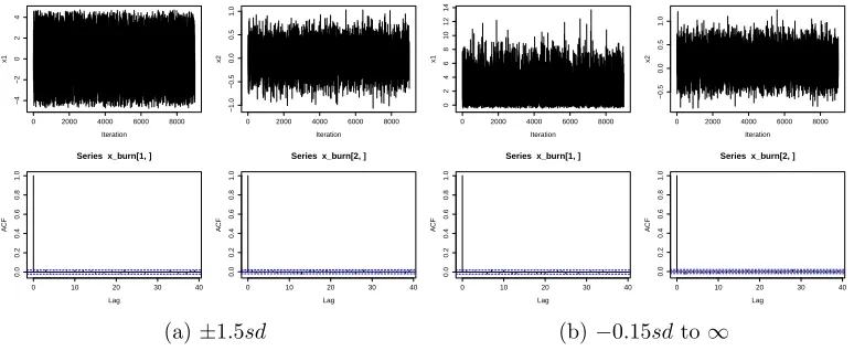
We generate 10,000 samples for every combination. Figures 3 and 4 display the contour

plots of the density function overlayed with the last 5,000 generated samples of the bounded

restriction region represented in case 1, and the one-sided open restriction region represented in

case 4, withρ= 0.5 and 0.98, respectively. It can be seen that the generated samples stay within

the restricted regions, and sample points distribute according to the steps of the contour lines,

which illustrates that the Gibbs sampler converges very fast to target distribution. Figures 3

and 4 also show that with higher correlation between the two components, the samples become

more concentrated on a line, while with lower correlation, the samples are more spread over the

plane.

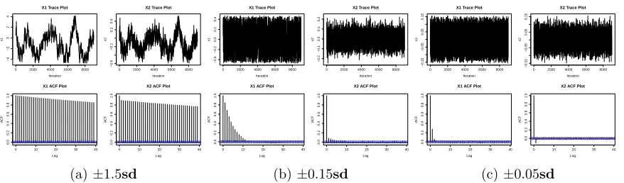
The mixing of a MCMC chain shows how fast the MCMC chain converges to the stationary

distribution. Trace plots and auto-correlation function(ACF) plots are good visual indicators of

the mixing property. These plots are shown in Figures 5 and 6 with 10,000 sample generations

−4 −2 0 2 4

−1.0

−0.5

0.0

0.5

1.0

(a)±1.5sd

0 5 10

−1.0

−0.5

0.0

0.5

1.0

(b)−0.15sdto ∞

Figure 3: Contour plots ρ= 0.5

−4 −2 0 2 4

−1.0

−0.5

0.0

0.5

1.0

(a)±1.5sd

0 5 10

0.0

0.5

1.0

1.5

(b)−0.15sdto ∞

Figure 4: Contour plotsρ= 0.98

correlation between the two components, the samples randomly cover the the marginal restriction

regions, and the auto-correlations decay to 0 very fast for both bounded and unbounded regions.

These illustrate that our Gibbs sampler has very good mixing property and the chains converge

fast to the true correct densities. For all cases, we also use the R function rtmvnormin package

tmvtnorm which is based on the Gibbs sampler proposed by Geweke (1991). However, for most

of the cases, especially unbounded restriction regions and wider bounded restriction regions,

show that this Gibbs sampler has very poor mixing property and the chains converge very slowly.

These plots are displayed in Figures 7 and 8.

0 2000 4000 6000 8000

−4 −2 0 2 4 Iteration x1

0 2000 4000 6000 8000

−0.6 −0.2 0.2 0.4 0.6 Iteration x2

0 10 20 30 40

0.0 0.2 0.4 0.6 0.8 1.0 Lag A CF

Series x_burn[1, ]

0 10 20 30 40

0.0 0.2 0.4 0.6 0.8 1.0 Lag A CF

Series x_burn[2, ]

(a)±1.5sd

0 2000 4000 6000 8000

−0.4 −0.2 0.0 0.2 0.4 Iteration x1

0 2000 4000 6000 8000

−0.2 −0.1 0.0 0.1 0.2 Iteration x2

0 10 20 30 40

0.0 0.2 0.4 0.6 0.8 1.0 Lag A CF

Series x_burn[1, ]

0 10 20 30 40

0.0 0.2 0.4 0.6 0.8 1.0 Lag A CF

Series x_burn[2, ]

(b)±0.15sd

0 2000 4000 6000 8000

−0.15 −0.05 0.05 0.15 Iteration x1

0 2000 4000 6000 8000

−0.15 −0.05 0.05 0.15 Iteration x2

0 10 20 30 40

0.0 0.2 0.4 0.6 0.8 1.0 Lag A CF

Series x_burn[1, ]

0 10 20 30 40

0.0 0.2 0.4 0.6 0.8 1.0 Lag A CF

Series x_burn[2, ]

(c)±0.05sd

Figure 5: Trace and ACF plots for 1-3 whenρ= 0.98

0 2000 4000 6000 8000

0 2 4 6 8 10 12 14 Iteration x1

0 2000 4000 6000 8000

0.0

0.5

1.0

Iteration

x2

0 10 20 30 40

0.0 0.2 0.4 0.6 0.8 1.0 Lag A CF

Series x_burn[1, ]

0 10 20 30 40

0.0 0.2 0.4 0.6 0.8 1.0 Lag A CF

Series x_burn[2, ]

(a)−0.15sdto ∞

0 2000 4000 6000 8000

2 4 6 8 10 12 Iteration x1

0 2000 4000 6000 8000

0.0 0.4 0.8 1.2 Iteration x2

0 10 20 30 40

0.0 0.2 0.4 0.6 0.8 1.0 Lag A CF

Series x_burn[1, ]

0 10 20 30 40

0.0 0.2 0.4 0.6 0.8 1.0 Lag A CF

Series x_burn[2, ]

(b) +0.15sdto∞

0 2000 4000 6000 8000

−10 −5 0 5 10 Iteration x1

0 2000 4000 6000 8000

−1.0 0.0 0.5 1.0 Iteration x2

0 10 20 30 40

0.0 0.2 0.4 0.6 0.8 1.0 Lag A CF

Series x_burn[1, ]

0 10 20 30 40

0.0 0.2 0.4 0.6 0.8 1.0 Lag A CF

Series x_burn[2, ]

(c)±∞

Figure 6: Trace and ACF plots for 4-6 whenρ= 0.98

0 2000 4000 6000 8000

−4

−2

0

2

4

X1 Trace Plot

Iteration

x1

0 2000 4000 6000 8000

−0.6

−0.2

0.2

0.4

X2 Trace Plot

Iteration

x2

0 10 20 30 40

0.0 0.2 0.4 0.6 0.8 1.0 Lag A CF

X1 ACF Plot

0 10 20 30 40

0.0 0.2 0.4 0.6 0.8 1.0 Lag A CF

X2 ACF Plot

(a)±1.5sd

0 2000 4000 6000 8000

−0.4

−0.2

0.0

0.2

0.4

X1 Trace Plot

Iteration

x1

0 2000 4000 6000 8000

−0.2

−0.1

0.0

0.1

0.2

X2 Trace Plot

Iteration

x2

0 10 20 30 40

0.0 0.2 0.4 0.6 0.8 1.0 Lag A CF

X1 ACF Plot

0 10 20 30 40

0.0 0.2 0.4 0.6 0.8 1.0 Lag A CF

X2 ACF Plot

(b)±0.15sd

0 2000 4000 6000 8000

−0.15

−0.05

0.05

0.15

X1 Trace Plot

Iteration

x1

0 2000 4000 6000 8000

−0.15

−0.05

0.05

0.15

X2 Trace Plot

Iteration

x2

0 10 20 30 40

0.0 0.2 0.4 0.6 0.8 1.0 Lag A CF

X1 ACF Plot

0 10 20 30 40

0.0 0.2 0.4 0.6 0.8 1.0 Lag A CF

X2 ACF Plot

(c)±0.05sd

0 2000 4000 6000 8000 0 1 2 3 4 5

X1 Trace Plot

Iteration

x1

0 2000 4000 6000 8000

−0.2

0.0

0.2

0.4

0.6

X2 Trace Plot

Iteration

x2

0 10 20 30 40

0.0 0.2 0.4 0.6 0.8 1.0 Lag A CF

X1 ACF Plot

0 10 20 30 40

0.0 0.2 0.4 0.6 0.8 1.0 Lag A CF

X2 ACF Plot

(a)−0.15sdto ∞

0 2000 4000 6000 8000

1 2 3 4 5 6

X1 Trace Plot

Iteration

x1

0 2000 4000 6000 8000

0.0

0.2

0.4

0.6

X2 Trace Plot

Iteration

x2

0 10 20 30 40

0.0 0.2 0.4 0.6 0.8 1.0 Lag A CF

X1 ACF Plot

0 10 20 30 40

0.0 0.2 0.4 0.6 0.8 1.0 Lag A CF

X2 ACF Plot

(b) +0.15sdto∞

0 2000 4000 6000 8000

−8 −6 −4 −2 0 2 4

X1 Trace Plot

Iteration

x1

0 2000 4000 6000 8000

−0.8

−0.4

0.0

0.4

X2 Trace Plot

Iteration

x2

0 10 20 30 40

0.0 0.2 0.4 0.6 0.8 1.0 Lag A CF

X1 ACF Plot

0 10 20 30 40

0.0 0.2 0.4 0.6 0.8 1.0 Lag A CF

X2 ACF Plot

(c)±∞

Figure 8: Trace and ACF plots for 4-6 when ρ= 0.98 by Geweke (1991)’s

Changing to a lower correlation between the two variables should improve the mixing

prop-erty and accelerate the convergence even more. However, since our Gibbs sampler already

performs extremely well, the improvement is not explicit whenρ = 0.5. The trace plots and the

ACF plots for some representative cases are given in Figure 9. This improvement is clearer when

using Geweke (1991)’s method, whose results are shown in Figure 10. However, although the

correlation is lowered to 0.5, the mixing property and the convergence for moderate truncated

restriction regions and the one-sided regions are still not very satisfactory as the trace plots are

sticky and the ACF’s decay to 0 fairly slowly.

0 2000 4000 6000 8000

−4 −2 0 2 4 Iteration x1

0 2000 4000 6000 8000

−1.0 −0.5 0.0 0.5 1.0 Iteration x2

0 10 20 30 40

0.0 0.2 0.4 0.6 0.8 1.0 Lag A CF

Series x_burn[1, ]

0 10 20 30 40

0.0 0.2 0.4 0.6 0.8 1.0 Lag A CF

Series x_burn[2, ]

(a)±1.5sd

0 2000 4000 6000 8000

0 2 4 6 8 10 12 14 Iteration x1

0 2000 4000 6000 8000

−0.5 0.0 0.5 1.0 Iteration x2

0 10 20 30 40

0.0 0.2 0.4 0.6 0.8 1.0 Lag A CF

Series x_burn[1, ]

0 10 20 30 40

0.0 0.2 0.4 0.6 0.8 1.0 Lag A CF

Series x_burn[2, ]

(b)−0.15sdto∞

Figure 9: Trace and ACF plots when ρ= 0.5

0 2000 4000 6000 8000 −4 −2 0 2 4

X1 Trace Plot

Iteration

x1

0 2000 4000 6000 8000

−1.0

−0.5

0.0

0.5

1.0

X2 Trace Plot

Iteration

x2

0 10 20 30 40

0.0 0.2 0.4 0.6 0.8 1.0 Lag A CF

X1 ACF Plot

0 10 20 30 40

0.0 0.2 0.4 0.6 0.8 1.0 Lag A CF

X2 ACF Plot

(a)±1.5sd

0 2000 4000 6000 8000

0 2 4 6 8 10

X1 Trace Plot

Iteration

x1

0 2000 4000 6000 8000

−1.0

−0.5

0.0

0.5

1.0

X2 Trace Plot

Iteration

x2

0 10 20 30 40

0.0 0.2 0.4 0.6 0.8 1.0 Lag A CF

X1 ACF Plot

0 10 20 30 40

0.0 0.2 0.4 0.6 0.8 1.0 Lag A CF

X2 ACF Plot

(b)−0.15sdto∞

Figure 10: Trace and ACF plots when ρ= 0.5 by Geweke (1991)’s

slow convergence caused by Geweke (1991)’s method. For every combination in this example,

we also compute the integrated auto-correlation time (IACT) for each individual chain. The

closer the IACT is to 1, the more effective the sampler is. The average of the IACT for all

of our combinations is 1.013, which is fairly close to 1. The CPU time for generating 10,000

samples using our Gibbs sampler for each combination is also recorded, and the average is

about 4.4 seconds on a DELL Dual Processor Xeon Twelve Core 3.6 GHz machines with 80GB

RAM running 64Bit CentOS Linux 5.0. The IACT and CPU time do not vary much when the

restriction regions and the correlations are changed. We also conduct the Geweke’s convergence

diagnosis test and all of the individual chains pass the tests. It is also worth pointing out that,

in our other simulation experiments, we discover that the Gibbs sampler proposed by us has a

better mixing property and faster convergence as the restriction regions become wider. However,

the above results show that our method still work satisfactorily for extremely tight truncation

restriction regions, and we have not found a case where our method has trouble converging. The

Gibbs sampler proposed by Geweke (1991) has a reverse trend, that is, it works better for tighter

restriction regions, however, this method becomes problematic for even moderately truncated

Example 2. In the description of our method, we claim that the linear constraint matrix Re

can have smaller rank than the dimension of the TMVN random vector. In this example, we

consider an 3-dimensional TMVN random vector X with mean and covariance matrix givenly

µ=       0 0 0      

, and Σ=

     

1 0.5 0.25

0.5 1 0.5

0.25 0.5 1

      .

The constraints with two types of restriction regions, bounded and one-sided open, are specified

as ˜ R=   

1 −2 0

−1 0 0





, c=

   0 0  

, and d =

   1 2   or    ∞ ∞   .

In examining the trace plots and the ACF plots with 10,000 generations and 1,000 burn-ins,

for both of the cases, our method has very good mixing property and converges fast to the true

density. However, for a 3-dimensional TMVN random vector, it is hard to display samples with

the contour plots of the true joint densities, or even the 2-dimensional marginal densities, as the

marginal distribution of a TMVN distribution is not TMVN, and the pdf has a very complex

expression. Therefore, to show the accuracy of our sampling method, we numerically compute

the 1-dimensional marginal density for each of the component for the two types of the restriction

regions. The numerical computation of the marginal densities involves evaluating the probability

of the restriction region and the density of a multivariate normal distribution, which is done by

employing the R packagemvtnorm. The histograms of our generated samples with the marginal

densities overlayed are given by Figures 11 and 12 for the bounded region and the one-sided

open region, respectively. These figures not only show that our Gibbs sampler gives a correct

and accurate sampling generation method, but also reveals the interesting effects resulted by

while those of X3 are symmetric and appear to be normally distributed, which is expected

because no constraints are imposed on X3. [provide the algm in Appendix?]

Histogram of x1

x1

Density

−2.0 −1.5 −1.0 −0.5 0.0

0.0

0.5

1.0

1.5

(a)x1

Histogram of x2

x2

Density

−1.5 −1.0 −0.5 0.0

0.0

0.5

1.0

1.5

(b)x2

Histogram of x3

x3

Density

−4 −3 −2 −1 0 1 2 3

0.0

0.5

1.0

1.5

(c) x3

Figure 11: The bounded region

Histogram of x1

x1

Density

−4 −3 −2 −1 0

0.0

0.2

0.4

0.6

0.8

(a)x1

Histogram of x2

x2

Density

−4 −3 −2 −1 0

0.0

0.2

0.4

0.6

0.8

(b)x2

Histogram of x3

x3

Density

−4 −3 −2 −1 0 1 2 3

0.0

0.2

0.4

0.6

0.8

(c) x3

Figure 12: The unbounded region

4.3

Sampling from TMVT

In this sub-section, we illustrate the empirical results of using our proposed Gibbs sampler in

sampling from TMVN distributions.

Example 3. We use the same µ, Σand Re as given in Example 1 for the TMVN distributed

random vector. In this example, we only display the results for two types of restriction regions,

with the lower bound−0.15sdand the upper bound +∞. We also set the correlation atρ= 0.5.

The degrees of freedom areν = 5. Figure 13 shows the trace and the ACF plots of 10,000 samples

with 1,000 burn-ins. These illustrate that our proposed Gibbs sampler for TMVT distributions

has good mixing property and fast convergence as the ACF’s decay to 0 very fast. The contour

plots overlayed with the last 5,000 samples are displayed in Figure 14. The plot for the

one-sided open region in Figure 14b is actually truncated as there are a few points generated at very

low density area. These clearly demonstrate that our sampling method successfully captures

the heavy-tailed nature of the multivariate Student-t distributions. Numerical examinations

shows that every individual chain in both of the cases has IACT approximately 1 and passes

the Geweke diagnosis tests.

0 2000 4000 6000 8000

−4 −2 0 2 4 Iteration x1

0 2000 4000 6000 8000

−2 −1 0 1 2 Iteration x2

0 10 20 30 40

0.0 0.2 0.4 0.6 0.8 1.0 Lag A CF

Series x_burn[1, ]

0 10 20 30 40

0.0 0.2 0.4 0.6 0.8 1.0 Lag A CF

Series x_burn[2, ]

(a)±1.5sd

0 2000 4000 6000 8000

−4 −2 0 2 4 Iteration x1

0 2000 4000 6000 8000

−2 −1 0 1 2 Iteration x2

0 10 20 30 40

0.0 0.2 0.4 0.6 0.8 1.0 Lag A CF

Series x_burn[1, ]

0 10 20 30 40

0.0 0.2 0.4 0.6 0.8 1.0 Lag A CF

Series x_burn[2, ]

(b)−0.15sdto +∞

Figure 13: Trace and ACF plots for TMVT ρ= 0.5 ν = 5

5

Conclusions

In this paper, we develop the sampling methods for both TUVN and TMVN distributions,

and generalize the methods to TMVT distributions. For TUVN distributions, we establish the

mixed rejection sampling method, utilizing four basic rejection sampling methods. For each

−4 −2 0 2 4

−2

−1

0

1

2

3

4

(a)±1.5sd

0 5 10 15 20 25 30 35

−2

−1

0

1

2

3

4

(b)−0.15sdto +∞

Figure 14: Contour plots for TMVT ρ= 0.5 ν= 5

sampling methods and select the one with the largest acceptance rate. Hence our method has

the optimized acceptance rate over the set of all restriction regions. Therefore our method is

more efficient than the existing widely used mixed rejection sampling methods by Geweke (1991)

and Robert (1995). For the TMVN distributions, we employ the Gibbs sampler taking

advan-tage of the distribution’s property that the full conditional distributions are still TMVN. Before

implementing the Gibbs sampler, a linear transformation is operated aiming to simplify the

functional form to a standard truncated multivariate normal distribution. This transformation

also contributes to fix the potential poor mixing property suffered by Geweke (1991)’s method.

Simulation studies show that our method has great accuracy, and good mixing property

regard-less of the type of the restriction regions. To obtain the samples from a general target TMVN

distribution, we only need a simple linear transformation after the Gibbs sampling is done. This

method is also computationally efficient as it only requires one matrix inversion on the Cholesky

decomposition of the covariance matrix. We generalize the method to sampling from TMVN

distributions as a multivariate Student-t distribution is a scale mixture density of a multivariate

normal density. The sampling method for the TMVT is also a Gibbs sampler with the Gibbs