How the EU Single Farm Payment should be modelled: lump-sum transfers, area payments or… what else?

How the EU Single Farm Payment should be modelled:

lump-sum transfers, area payments or… what else?

Frédéric COURLEUX, Hervé GUYOMARD, Fabrice LEVERT, Laurent PIET

Working Paper SMART – LERECO N°08-01

May 2008

UMR INRA-Agrocampus Ouest SMART (Structures et Marchés Agricoles, Ressources et Territoires) UR INRA LERECO (Laboratoires d’Etudes et de Recherches Economiques)

How the EU Single Farm Payment should be modelled:

lump-sum transfers, area payments or… what else?

Frédéric COURLEUX

Ministère de l’Agriculture et de la Pêche, F-75000 Paris, France

Hervé GUYOMARD

INRA, UAR233 Collège de Direction, F-75000 Paris, France

Fabrice LEVERT

INRA, UMR1302 SMART, F-35000 Rennes, France Agrocampus Ouest, UMR1302 SMART, F-35000 Rennes, France

Laurent PIET

INRA, UMR1302 SMART, F-35000 Rennes, France Agrocampus Ouest, UMR1302 SMART, F-35000 Rennes, France

At the time of writing, Frédéric Courleux was a member of INRA as a PhD student in the UMR1302 SMART.

Auteur pour la correspondance / Corresponding author Laurent PIET

INRA, UMR SMART

4 allée Adolphe Bobierre, CS 61103 35011 Rennes cedex, France

Email: [email protected]

Téléphone / Phone: +33 (0)2 23 48 53 83 Fax: +33 (0)2 23 48 53 80

How the EU Single Farm Payment should be modelled: lump-sum transfers, area payments or… what else?

Abstract

The 2003 Common Agricultural Policy (CAP) reform radically changes the way the European Union (EU) supports its agricultural sector by decoupling direct payments. Production is no longer required to get the payment attached to Single Farm Payment (SFP) entitlements. However, the new scheme maintains a specific link between payments and hectares; in addition, SFP entitlements can be exchanged among farmers. These features question the way SFP entitlements should be regarded, hence modelled, i.e., as lump-sum transfers, area payments or… something else. We develop a microeconomic analytical framework which shows that the answer crucially depends on the total number of entitlements which are initially made available relative to the number of hectares, more specifically the number of cultivated hectares in a zero support regime, the number of cultivated hectares in a policy support regime trough per-hectare direct aids, and the number of cultivated or idled hectares in a policy regime where support is granted through direct aids per hectare and production is not required.

Keywords: European Union, Common Agricultural Policy, Single Farm Payment, modelling, area payments, lump-sum transfers

JEL Classification: Q18, Q12

Comment modéliser les Droits au Paiement Unique de l’UE : transferts forfaitaires, aides à l’hectare ou… quoi d’autre ?

Résumé

Le découplage des paiements directs adopté lors de la réforme de la Politique Agricole Commune (PAC) de 2003 modifie radicalement la façon dont l’Union Européenne (UE) soutient son secteur agricole. Il n’y a plus d’obligation de production pour pouvoir prétendre au bénéfice de l’aide attachée aux Droits au Paiement Unique (DPU). Malgré cela, le nouveau

dispositif maintient un lien spécifique entre les paiements et la terre ; de plus, les DPU peuvent être échangés entre agriculteurs. Etant donné ces caractéristiques, la question de la modélisation des DPU se pose : sont-ils des transferts forfaitaires, des aides à la surface ou… autre chose ? Le cadre analytique microéconomique proposé ici montre que la réponse dépend fondamentalement du rapport entre le nombre total de droits mis en circulation à l’initialisation du dispositif et, premièrement, le nombre d’hectares qui seraient cultivés en l’absence de tout soutien, deuxièmement, le nombre d’hectares qui seraient cultivés en présence d’aides directes à l’hectare, et troisièmement, le nombre d’hectares qui seraient cultivés ou laissés en gel volontaire en présence d’aides directes à l’hectare sans obligation de production.

Mots-clefs : Union Européenne, Politique Agricole Commune, Droit au Paiement Unique, modélisation, aides à la surface, transferts forfaitaires

How the EU Single Farm Payment should be modelled: lump-sum transfers, area payments or… what else?

1. Introduction

On 26 June 2003, European Union (EU) farm ministers adopted a new reform of the Common Agricultural Policy (CAP). This reform radically changes the way the EU supports its agricultural sector. Among the various features characterizing the horizontal Council Regulation (EC) 1782/2003 (essentially modulation, financial discipline, cross-compliance criteria and new rural development measures), the decoupling of direct payments granted through the so-called first pillar appears to be the most at odds with the previous policy inherited from the 1992 and 1999 reforms.1 It is implemented through a Single Payment Scheme (SPS) which mitigates into a Single Farm Payment (SFP) a majority of the direct aids that were formerly granted per hectare (cereals, oilseeds and protein crops) and/or per animal head (beef, veal, sheep and goats).2

The SFP is broken down into a certain number of entitlements which in practice correspond to unit amounts of aids per hectare in so far as each entitlement has to be “accompanied by an eligible hectare” in order to “give right to the payment of the amount fixed by the payment entitlement” (EC 1782/2003, article 44). As a result, one could regard SFP entitlements simply as area payments. However, a second feature of the SPS makes SFP entitlements

potentially different from area payments. Whatever the national implementation model,3

actual production of a specific commodity among those which are eligible is no longer

1

The first pillar of the CAP corresponds to traditional market support measures (export subsidies, intervention spending, etc.) and direct payments (including the Single Farm Payment scheme introduced in 2003). Rural development, agri-environmental and other accompanying measures define the second pillar

2

The SPS also includes components originating from dairy and sugar beet payments which were introduced in 2004 and 2006, respectively, in order to compensate for intervention price cuts in the milk and sugar sectors. From 2005 on, it includes payments granted to tobacco, cotton and olive oil. The 2007 reform of the Common Market Organisation (CMO) in fruit and vegetables integrates these products into the SPS. For details on these successive reforms, see the website of the European Commission (http://ec.europa.eu/agriculture/index_en.htm). 3

The reader is referred to the European Commission website for a detailed presentation of the 2003 CAP reform. In particular, Council Regulation (EC) 1782/2003 and Commission Regulations (EC) 795/2004, 796/2004 and 118/2005 define the legal basis for direct payments, notably the various models (historic, regional or hybrid) a Member State can use for implementing the SPS.

required to get the payment attached to entitlements, provided cross-compliance conditions

are met on the corresponding hectares.4 From that perspective, one could be inclined to look

at the SFP as a lump-sum transfer to the farmer.

From the previous presentation, a difficulty immediately arises. As noted by Bascou et al. (2004), “(t)he way in which the single farm payment is implemented and modelled may notably influence producer decisions and the projected production patterns”. Though a model is clearly a simplification of reality, it is always most desirable to adopt an as explicit as possible representation of policies in models. This is the main objective of this paper which tries to bring some clarity into the debate on the way SFP entitlements should be modelled, more specifically as lump-sum transfers, area payments or… something else. To do so, we develop a simplified microeconomic production framework to compare three situations corresponding to, respectively, (i) a zero support regime, (ii) a regime where support is granted through direct aids per hectare and (iii) a regime where support is granted through the

SPS.5 The analytic approach we develop integrates the three main characteristics of the SPS

that make payments a priori different from both lump-sum transfers and area subsidies. First,

production is no longer required to get payments attached to entitlements. Second, the scheme maintains a specific link between payments and hectares through the so-called “activation constraint”, i.e., the obligation for a farmer to maintain in potential agricultural use (through the respect of Good Agricultural and Environmental Conditions (GAECs)) a number of eligible hectares at least equal to the number of SFP entitlements he holds to get the payment

attached to the latter.6 Third, SFP entitlements can be exchanged among farmers, necessarily

with a concomitant and equivalent land transfer in the case of a temporary entitlement transaction, with or without land transfer if the entitlement transaction is permanent.

The rest of the paper is structured as follows. Section 2 briefly reviews researches that used one of the two options described above (lump-sum transfers or area payments) to represent

4

That is as long as the farmer complies with environmental, animal and plant health, animal welfare and food safety standards, as well as he maintains land in Good Agricultural and Environmental Conditions.

5

Farmers are profit maximizers, there is no uncertainty and all markets are competitive. Hence the zero support regime also depicts a situation where agricultural income support is granted through lump-sum transfers (except that agricultural income is increased by an amount equal to these lump-sum transfers).

6

Article 44.3 of the Council Regulation (EC) 1782/2003 specifically stipulates that “the parcels shall be at the farmer’s disposal for a period of at least 10 months” of the cropping year during which the payments are applied for.

the SFP. Section 3 details our modelling framework; we first describe the zero support regime; we then bring in direct aids per hectare equivalent to those which were in place in the EU sector of cereals, oilseeds and protein (COP) crops from the 1992 CAP reform until 2003;7 finally, direct aids per hectare are replaced by SFP entitlements. The concluding section summarises our findings and discusses their implications on how SFP entitlements should be represented in models.

2. How has the Single Payment Scheme been modelled so far? The lump-sum transfer solution

Several authors have modelled the SFP as a lump-sum transfer granted to agricultural households. In a partial equilibrium (PE) setting (FAPRI-Ireland Partnership, 2003; Bascou et al., 2004; Breen et al., 2005; Schmid et al., 2006), such a transfer cannot be explicitly accounted for since the income formation of households is not modelled; as a result, the amount corresponding to the SFP simply accounts for zero in the profit maximisation behavior of agricultural producers. Under this assumption, the 2003 CAP payments have no impact at all on farmers’ production decisions, input use (especially land demands) and output supply (especially yields).

In a general equilibrium (GE) setting (Gohin, 2004; Gelan and Schwarz, 2006), the income formation of consumers is modelled and the lump-sum transfer equivalent to the total amount of the SFP is explicitly introduced as accruing to households. Within this framework, the production-decision side is not affected by the SFP. Nevertheless, a certain wealth effect can come into play on the consumption side in so far as the increase in consumers’ income can affect their decisions in terms of both resource allocation and income spending. It should be noted though that, in the examples cited above, agricultural households are not explicitly accounted for, as only a single representative consumer agent is considered. As a result, the SFP is “diluted” as if it were a very generic transfer to all households, agricultural households as well as non-agricultural households.

7

Per-hectare direct aids granted to COP crops can be maintained in Member States which decide to decouple only partially in the COP sector. However, unit per-hectare amounts are considerably reduced with respect to pre-2003 levels. Only France and Spain chose to maintain the support in the COP sector partially coupled.

In short, when the new EU payments are modelled as lump-sum transfers, they de facto do not affect output supply and input use, in particular the land demand addressed by farmers to land owners. They do not capitalize into land prices and rents. Models that have adopted this first approach effectively conclude that decoupling should result in land rents to decrease sharply relative to the pre-2003 situation, e.g., -80 % in Gohin (2004).

The area payment solution

The second approach adopted by modellers is to consider SFP entitlements just as if they were area payments. This alternative solution has been adopted in PE models (Junker et al., 2003; Binfeld et al., 2003; Binfeld et al., 2004; Huettel et al., 2005; Balkhausen et al., 2005; Buysse et al., 2007) and GE frameworks (Frandsen et al., 2003; Jensen and Frandsen, 2004; Gohin, 2004, 2006).8 It is not our purpose here to discuss whether area payments such as those in place in the EU COP sector since 1992 have been satisfactorily or not represented in models so far. However, we do need to briefly describe how they have been actually modelled in order to understand implications regarding the effects of SFP entitlements when they are introduced as area payments.

Most PE models do not explicitly represent factor markets, notably the land factor market. Even when they include a land allocation mechanism, and hence product-specific land derived demand equations, they generally do not compute equilibrium land rental prices which could enter these land demand functions. As a result, it is not possible to specify land demand equations in which the land price net of the area payment could be an explicit argument. To overcome this limitation, area payments are then introduced as a complement to the output price in equations that determine the areas devoted to each eligible crop.9 In order to account for the fact that the supply-inducing effects of area payments are less than the impacts of output price support, the OECD AGLINK model multiplies area payments by a coupling factor of 0.14 (OECD, 2004). As noted by Gohin (2006), only the OECD justifies the value retained for the coupling factor relying on a policy simulation analysis performed with the

8

Gohin (2004, 2006) is actually one of the few who compares the effects of considering 2003 EU payments as either lump-sum transfers or area subsidies.

9

Policy Evaluation Model (PEM) which integrates the land market (Dewbre et al., 2001)10 The value of the coupling factor adopted in other PE models is not justified. In practice, it varies between zero and one reflecting essentially a priori believes of modellers (Gohin, 2006; Balkhausen et al., 2007).

By contrast, GE models do represent the land market. Area payments can then be explicitly introduced in agricultural land demand equations by lowering the endogenous rental price of land. In a general way, GE models allocate land according to constant elasticity of transformation (CET) functions which capture the constrained mobility of total available land among competing uses. As a result, there are several land rental prices reflecting the fact that land is, in practice, a heterogeneous production factor. GE models, as well as PE models which explicitly include the land market, can be used to address the issue of agricultural support capitalisation into land prices and rents. They however suffer from two main drawbacks. First, their agricultural area coverage is incomplete since in many cases, several agricultural land uses are not included (fodder and pasture area, voluntary set-aside area, etc.). In addition, the models’ product aggregation is not always fully consistent with the one retained by policymakers. Second, as rightfully pointed out by Gohin (2006), EU land rental

prices net of per-hectare direct payments are generally negative.11 Gohin (2006) explains this

very partial capitalisation of area payments into land prices by two factors: land price capitalisation takes time in particular because land-leasing contracts are long-term arrangements that are very difficult to renegotiate; there are rigidities and imperfections in agricultural production factor markets, not only the land market, due to notably national regulations on farmland uses and prices, but also the labour and capital markets. Accordingly, Gohin (2006) argues that it is not unreasonable to model pre-2003 area payments, for a part as land subsidies, for the remaining as labour/capital subsidies. In his empirical analysis, he assumes an equal sharing. He immediately recognizes that this choice is somewhat arbitrary.

10

By contrast to other PE models, the PEM developed by the OECD includes a land market modelling which is very similar to the one adopted in GE frameworks.

11

See also von Witzke et al. (2007) who conclude that in a typical German farm, the 2005/06 land rental price would be negative in the absence of agricultural subsidies.

Let us now consider how SFP entitlements are dealt with in simulation models where they are introduced as area payments. Under this assumption, the 2003 CAP decoupling is depicted as a switch from area payments restricted to COP crops, as well as mandatory set-aside, to non-product-specific direct aids per hectare for all eligible areas. In the AGLINK model for example, the SFP affects only the first stage of the three-step area allocation system, i.e., the decision relating to the choice between the total area for cereals and oilseeds on the one hand, the total area for fodder crops and pasture on the other hand. Subsequent area allocation decisions depend only on relative returns (OECD, 2004). To reflect the lower degree of SFP entitlements as compared to the pre-2003 area payments, the coupling factor is now set to 0.06 (instead of 0.14 for area payments). This lower figure is based on Dewbre et al. (2001) who showed that area payments requiring planting of specific crops are slightly more trade distorting than payments not requiring planting of specific crops. The other models which also adopt the coupling factor approach do not justify the choice of the coefficient ascribed to SFP entitlements. The coefficient is generally assumed lower than the one associated with pre-2003 area payments (0.15 versus 0.50 for the FAPRI-GOLD model, Binfield et al., pre-2003; Binfield et al., 2004), but it is sometimes maintained unchanged (1 for the ESIM model, Balkhausen et al., 2005).12

3. The microeconomic framework

The microeconomic framework developed below takes explicitly into account the three main characteristics of the 2003 EU SPS, i.e., (i) the activation constraint, (ii) the free tradability of SFP entitlements and (iii) the fact that production is no longer required but cross-compliance criteria apply. The model is developed progressively. In a first step, we introduce the two first characteristics (section 3.3). In the second step, we add the third feature (section 3.4). We begin the presentation by defining the two comparison regimes, i.e., first the zero support regime or, equivalently here, the lump-sum transfer regime (section 3.1), second a regime of per-hectare direct aids (section 3.2). It is from this comparison that we will derive implications on how SPF entitlements should be modeled.

12

3.1. The zero support regime

We consider a two-producer agricultural economy. Each farmer i=1,2 maximizes his profit

according to the following program:

) , , , ( )] , , ( ; [ max_x,h p_iy_i −wx_i −rh_i y_i = f_i x_i h_i l_i ≡θ_i p_i w r l_i , (1) where p_i is the output price, y_i is the output level, w is the vector of variable input prices,

i

x is the vector of variable input quantities, r is the land rental price, h_i is the land quantity, )

, , ( _{i i i}

i x h l

f is a well-behaved production function with l_i the (fixed) family labour endowment of farmer i.

We retain three simplifying assumptions in order to make things manageable and analytical results more easily interpretable. These assumptions do not alter general conclusions of our analysis. First, output and variable input equilibrium prices are assumed exogenous and constant.13 Second, land is acquired or let through rental only; the buying or selling price of land is assumed to be adequately approximated by the discounted sum of future rental values so that a prediction about the direction of the land rental price is equivalent to a prediction about the direction of the buying or selling land price (Leathers, 1992). Finally, land endowments of farmers are supposed null.

Program (1) defines a profit function

θ

_i(p_i,w,r,l_i) which is assumed twice continuously differentiable, non negative, non decreasing in output price, non increasing in input prices, non decreasing in family labour quantity, linearly homogeneous and convex in prices, and concave in family labour quantity (Diewert, 1974). The land demand function for farmer i is obtained by differentiation of his profit function with respect to the land rental price (Hotelling’s lemma): r l r w p l r w p h_i( _i, , , _i)≡−∂

θ

_i( _i, , , _i)/∂ . (2)

The land market equilibrium is then defined by equating farmers’ land demands to land supply, i.e., ) ( ) , , , ( 2 1 wp i i wp i i p w r l L r h

∑

= = , (3) 13

where L(r) is the land supply function to the farm sector by landowners, with ∂L(r)/∂r≥0. Equation (3) solved for r defines the equilibrium land rental price, rwp, as a function of output and variable input prices, as well as family labour endowments.

The land market is depicted in Figure 1 where equilibrium occurs at point _Ewp_{, for an}

equilibrium land rental price of rwp. For this equilibrium land rental price, farmer 1 leases in the land quantity h₁wp ≡h₁(p₁,w,rwp,l₁) and farmer 2 leases in the land quantity

) , , , ( _{2 2} 2 2 h p w r l hwp ≡ wp _.

3.2. Introducing directs aids per hectare

In a regime where agricultural income support is granted through direct aids per hectare, program (1) becomes: ) , , , ( )] , , ( ; [ max_x,h p_iy_i−wx_i −rh_i+a_ih_i y_i = f_i x_i h_i l_i ≡

θ

_i p_i w r−a_i l_i , (4) where a_i denotes the per-hectare direct aid for farmer i.14

As in the case of zero support, the land demand function of each farmer is defined by the derivative of the profit function with respect to the land rental price, and the land market equilibrium is obtained when aggregate demand for land equals land supply:

) ( ) , , , ( / ) , , , ( 2 1 2 1 a i i i a i i i i i a i i p w r a l r

∑

h p wr a l L r

∑

= = = − = ∂ − ∂ − θ . (5)

where the superscript a denotes equilibrium variables in a support regime of per-hectare direct aids.

14

We do not constrain per-hectare direct aids to be equal for the two farmers since we do not impose that they both produce the same output (see note 13). However, we do not allow a given farmer to shift, even partially, from one production to another.

Figure 1. The land market equilibrium in the zero support regime. wp E wp 2 h wp 1 h wp H wp r ) (r L r r δ δθ1( )/ − r r δ δθ₂( )/ − ∑ = − 2 , 1 / ) ( i i r δr δθ Prices, costs Quantities

The comparative static of the land rental equilibrium price in this policy regime is determined by totally differentiating (5) and solving for dra:15

] / / [ . / 2 2 1 2 2 1 2 2 r L r da r dr i i i i i a ∂ ∂ + ∂ ∂ ∂ ∂ =

∑

∑

= = θ θ . (6)

The response of individual land demands to changes in per-hectare direct aids is obtained by differentiating each derived land demand function h_i(p_i,w,r−a_i,l_i), evaluated at equilibrium land rental price, with respect to direct aids. For farmer 1 one yields:

). ] / / [ . / ) ( . / ( . / ) ] / / [ . / ( . / ) ( . / 2 2 1 2 1 1 2 2 2 2 2 1 2 1 2 2 1 2 2 1 2 2 2 1 2 1 2 1 2 1 r L r da r L da da r r da r L r da r r da dr r dh i i i i i i i a a ∂ ∂ + ∂ ∂ ∂ ∂ − − ∂ ∂ ∂ −∂ = − ∂ ∂ + ∂ ∂ ∂ ∂ ∂ −∂ = − ∂ −∂ =

∑

∑

∑

= = = θ θ θ θ θ θ θ (7)

Equation (7) shows that per-hectare direct aids granted to the first product (equivalently here the first producer) have a positive impact on land allocated to the first product (positive own-aid effect). By contrast, per-hectare direct own-aids granted to the second product (equivalently here the second producer) have a negative impact on land allocated to the first product (negative cross-aid effect).

The response of total land demand to changes in per-hectare direct aids is readily obtained as the sum dHa =dh₁a +dh₂a: ] / / [ . / . / 2 2 1 2 2 1 2 2 r L r da r r L dH i i i i i a ∂ ∂ + ∂ ∂ ∂ ∂ ∂ ∂ =

∑

∑

= = θ θ . (8) 15

Equation (6) assumes that output and variable input prices, as well as family labour endowments, are kept constant. One easily shows that the equilibrium land rental price is an increasing function of output prices and, as a result, that an output price support policy also capitalizes, at least partially, into land prices.

In the case where the land supply function is not perfectly inelastic (∂L/∂r >0), per-hectare direct aids are coupled at the extensive margin of production since they increase aggregate land used in the farm sector. In the specific case where the land supply function is perfectly inelastic (∂L/∂r =0), they have no impact on aggregate land used in the farm sector.

We summarise the previous analysis by the following proposition.

Proposition 1. Direct aids per hectare capitalize at least partially in land prices. The lower the land supply elasticity, the higher the capitalization in land prices. Capitalization is complete when per-hectare direct aids are identical for all outputs and the land supply function is perfectly inelastic. Own effects of per-hectare direct aids are positive and cross effects are negative. Except in the specific case where the land supply function is perfectly inelastic, direct aids per hectare increase total land used in the farm sector.

3.3. The SPS assuming that production is required

Producer maximization program

In the SFP policy regime, each producer maximizes his profit according to the following program: ] 0 ; ) , , ( ; ) ( [ max_x,h,n p_iy_i −wx_i −rh_i+bn_i−v n_i −n_i0 y_i = f_i x_i h_i l_i ≤n_i ≤h_i , (9a) where b is the unit value of payment entitlements, n_i is the number of entitlements for farmer

i, v is the rental price of entitlements, and n_i0 is the initial entitlement endowment for farmer

i. For convenience, payment entitlements are assumed to be acquired or let through rental only. For the sake of simplicity, we also consider that they exhibit the same unit value b

whatever the farmer.16

16

This assumption does not alter our findings regarding the modelling of the SPS. When unit values of SFP entitlements differ among farmers, we have to consider as many entitlement rental prices as entitlement unit values. However, one shows that equilibrium entitlement rental prices then verify b_i −v_i =d ≥0, where d is a non-negative common value, whatever the farmer i (intuitively, this occurs to exhaust arbitration possibilities, i.e., the possibility for a farmer, say 1, to make a gain by selling his equilibrium entitlement demand and buying the same quantity from another farmer, say k, in a situation where v₁ −b₁ >v_k −b_k). All the results derived in the text remain valid since, as we will show, what matters in behavioural and equilibrium equations is the difference b_i −v_i for all farmers i.

From equation (9a), one sees that the SPS induces three main differences in the producer maximisation program with respect to the regime of direct aids per hectare (equation (4)). First, total payments received by farmer i are no longer proportionate to the number of hectares h_i he demands but to the number of entitlements n_i he claims for. Second, the difference v(n_i−n_i0) represents either the costs of renting in additional payments at a price v per unit or the earnings of renting out part or all of the initial payment endowment, also at a price v per unit; this accounts for the tradable nature of SFP entitlements. Third, the inequality constraint n_i ≤h_i captures the fact that payments are granted only for entitlements for which the farmer i holds an eligible hectare; this is the way we represent the “activation constraint”.

Program (9a) can equivalently be written as:

] 0 ; ) ( ) , , , ( [ max_h,n

π

_i p_i w h_i l_i −rh_i+bn_i −v n_i−n_i0 ≤n_i ≤h_i , (9b) where π_i(p_i,w,h_i,l_i) is a well-behaved profit function defined for a given land quantity:

)] , , ( ; [ max ) , , , ( _{i i i x i i i i i i i i} i p w h l ≡ p y −wx y = f x h l π . (9c)

The first-order necessary conditions for program (9b) are: 0 / ) ( ∂ − + = ∂π_i h_i h r λ , (10a) 0 = − + −v µ λ b , (10b) 0 .n_i = µ , (10c) 0 ) ( . h_i−n_i = λ , (10d)

where µ and λ are the Lagrange multipliers associated with the inequality constraints 0≤n_i

Land and entitlement demand functions

Equations (10a) to (10d) allow deriving the land demand function and the entitlement net demand function for farmer i as follows.17 Let us first assume that v<b. Under this assumption, λ >0 (from (10b)), n_i =h_i (from (10d)), µ =0 (from (10c) and because we focus on the case where h_i >0) and ∂π_i(h_i)/∂h=r+v−b (from (10a)). Let us now assume that v=b. Under this assumption, µ =λ=0 (from (10b), (10c) and (10d)), ∂π_i(h_i)/∂h=r

(from (10a)) and 0≤n_i ≤h_i. Finally, let us assume that v>b. Under this assumption, µ >0 (from (10b)), n_i =0 (from (10c)), λ =0 (from (10d)) and ∂π_i(h_i)/∂h=r (from (10a)). To sum up:

when v<b, ∂π_i(h_i)/∂h=r+v−b and n_i =h_i, (11a) when v=b, ∂π_i(h_i)/∂h=r and 0≤n_i ≤h_i, (11b) when v>b, ∂π_i(h_i)/∂h=r and n_i =0. (11c)

Land and entitlement market equilibriums

Let us now turn to land and entitlement market equilibriums. The land market equilibrium requires that aggregate land demand equals aggregate land supply. The entitlement market equilibrium condition requires that the total number of entitlements activated by farmers is lower than or equal to the global endowment in entitlements denoted N0. Three regimes have to be distinguished depending on whether N0 ≤Hwp_, wp b

H N

H ≤ 0 ≤ _{, or H}b _≤N0

, where

wp

H is total agricultural land used in the zero support reference situation and _Hb _{is the}

number of hectares which would be demanded in a support regime of per-hectare direct aids of unit amount equal to the entitlement unit value b. Annex details why these three regimes have to be considered.

17

The analysis excludes the uninteresting case where the land rental price is so high that the marginal profit of the first hectare is lower than the land rental price. In other words, as previously noted, we only consider the case where h_i >0.

Regime 1. N0 ≤ Hwp =L(rwp)

In that first regime, the initial number of entitlements is lower than or equal to the number of hectares which would be demanded in the zero support policy reference situation. One then shows that market equilibrium conditions may be defined as (proof in Annex 1):

b vs = , (12a) r l r w p l r w p h h_is = _i( _i, , s, _i)=−∂θ_i( _i, , s, _i)/∂ , (12b) ) ( ) , , , ( 2 1 s i i s i i p w r l L r h =

∑

= , (12c) s i s i h n ≤ , (12d) wp i s i N H n = ≤

∑

= 0 2 1 , (12e)

where the subscript s denotes equilibrium variables in this first SFP regime.

In that first regime, the equilibrium rental price of entitlements equals the unit value of entitlements (equation (12a)). With respect to the zero support situation, the SFP scheme has no impact on individual land demands (equation (12b)), the aggregate land quantity used in the farm sector and the land rental price (equation (12c) which is identical to equation (3)). The total number of payment entitlements effectively used by the farmers is equal to the initial endowment in entitlements (first part of equation (12e)). There are entitlement exchanges from the over-endowed farmer (if he exists) towards the under-endowed farmer (if he exists).18 Both the over-endowed farmer and the under-endowed farmer gain from exchanging payment entitlements relative to a regime where entitlements cannot be exchanged. This can be shown graphically as follows.

Figure 2 corresponds to the limit case where N0 =Hwp. In the zero support regime, farmer 1 demands _h1wp =_h1(_rwp) _{hectares and farmer 2 demands ( )}

2 2 wp wp _{h r} h = hectares with ). ( 2 1 wp wp wp wp r L H h

h + = = Initial endowments in entitlements are n₁0 >h₁wp and n₂0 <h₂wp

such that n₁0 +n₂0 =N0 =Hwp.

18

A farmer will be said over-endowed (respectively under-endowed) when his initial endowment in entitlements is strictly higher (lower) than the number of hectares he would demand under a zero support regime.

Figure 2. The land market equilibrium in the SFP support regime without the possibility not to produce when the number of

entitlements N0 is lower than or equal to the number of hectares demanded in a zero support regime (a).

A G C D I K J L F H B α γ ψ ε δ β η sne E wp E 0 2 n h2sne s 2 wp 2 h h = s 1 wp 1 h h = _N0_=Hwp_=Hs sne 1 h 0 1 n Hsne sne r wp r M O N b b ) (r L Z X Y ξ P Prices, costs Quantities

(a) The case illustrated is the limit case where N0 =Hwp (where Hwp is the total area demanded in a zero support regime). The superscripts s and sne denote equilibrium variables, respectively when SFP entitlements are tradable and when they cannot be exchanged.

(i) Let us first assume that payment entitlements cannot be exchanged. Under this assumption, the aggregate land demand curve is represented by the broken line ABCDEsneXYZ (i.e., the horizontal sum of demand curves αβδεηξ and ABFMOP). The land market equilibrium occurs at point Esne (where the superscript sne denotes equilibrium variables in this regime of non-tradable SFP entitlements) where land demand and supply curves intersect. The land rental price increases from rwp to rsne, and land used in the farm sector increases from

) ( wp

wp

r L

H = to Hsne =L(rsne). With no trade in entitlements, the SFP scheme results in an increase in total land used in the farm sector; the over-endowed farmer 1 increases his land demand to _hsne

1 where h h r b

sne sne ∂ = −

∂π₁( ₁ )/ while the under-endowed farmer 2 decreases his land demand to h₂sne where ∂π₂(h₂sne)/∂h=rsne. With respect to the zero support regime, farmer 1 unambiguously gains because area AFJG is greater than area IJLK.19 Farmer 2 gains area αβδγ but looses area IεηK, the net outcome depending on whether area αβδγ is greater or smaller than area IεηK. The over-endowed farmer 1 does not use all his initial endowment in entitlements, and the under-endowed farmer 2 demands a number of hectares greater than his initial entitlement endowment.

(ii) Let us now assume that payment entitlements can be exchanged. Under this assumption, the aggregate land demand is the broken line GNEwpYZ and there is no impact on the land market: the equilibrium land rental price is _rs =_rwp_{, individual land demands are h}s _hwp

1 1 = for

farmer 1 and h₂s =h₂wp for farmer 2, and total land used in the farm sector is Hs =Hwp (where the superscript s denotes equilibrium variables in this regime of tradable SFP). The SFP scheme is decoupled at the extensive margin of production. The over-endowed farmer 1 leases out the entitlement quantity n₁0−h₁s at price ν =b which is leased in by the under-endowed farmer 2. With respect to the zero support regime, the over-under-endowed farmer 1 gains area AMOG. With respect to the non tradable SFP regime, he gains IJLK +JFMO. With respect to the zero support regime, the under-endowed farmer 2 gains area αβδγ . With respect to the non tradable SFP regime, he gains IεηK. Relative to the non tradable regime, both producers thus benefit from exchanging payment entitlements.

The following proposition summarizes the previous analysis.

19

Proposition 2. When the initial number of payment entitlements is lower than or equal to the number of hectares that farmers would demand in a zero support regime, introducing tradable single farm payments has no impact on the land market: the land rental price, the total agricultural area and farmers’ land demands are unchanged. All payment entitlements are activated, and there are entitlement exchanges from the over-endowed farmer (if he exists) towards the under-endowed farmer (if he exists).

Regime 2. Hwp =L(rwp)≤N0 ≤ Hb

In that second regime, the initial number of entitlements is greater than or equal to the number of hectares which would be demanded in the zero support policy scenario (Hwp ≤N0), and lower than or equal to the number of hectares which would be demanded in a regime where support would be granted through direct aids per hectare of unit amount b (N0 ≤Hb where

b H is defined by ( , , , ) ( ) 2 1 b i i b i i b r L l b r w p H =

∑

−∂ − = = θ

). In that case, equilibrium conditions may be written as (proof in Annex):

b vs ≤ ≤ 0 , (13a) r l b v r w p l b v r w p h h s s _i i i i s s i i s i = ( , , + − , )=−∂θ ( , , + − , )/∂ , (13b) 0 ) (r N L s = _{, (13c)} ) ( ) , , , ( 2 1 s i i s s i i p w r v b l L r h + − =

∑

= , (13d) s i s i h n = , (13e) b i s i wp _{n N H} H ≤

∑

= ≤ = 0 2 1 . (13f)

In that second regime, the equilibrium rental price of entitlements is lower than or equal to their unit value (equation (13a)). SFP entitlements now have an impact on individual land demands (equation (13b)). Equation (13d) defines the equilibrium entitlement price for a given equilibrium land rental price defined by equation (13c). One easily verifies that

wp s _r

on land and entitlement equilibrium prices are obtained by differentiating equations (13c) and (13d) with respect to N0: 1 0 ) / ( /dN = ∂L ∂r − drs , (14a) ] ) / ( ) / [( /dN0 =− ∂L ∂r −1+

∑

∂ ∂r −1 dv

θ

_i . (14b)

An increase in the number of entitlements raises the land rental price (equation (14a)) and diminishes the entitlement rental price (equation (14b)). The equilibrium land rental price is thus an increasing function in the number of payment entitlements, rising from rs =rwp when

wp

H

N0 = to rs =rb when N0 =Hb. The equilibrium entitlement rental price is a decreasing function in the number of payment entitlements, diminishing from vs =b when

wp

H

N0 = to vs =0 when N0 =Hb.

From equation (13b), one verifies that individual land demands increase with the total number of entitlements because: 0 ) / ( / / 1 2 1 0 0+ =− ∂ ∂ − < =

∑

i i s r dN dv dN dr θ , (15) and hence, 0 ) / / ( . / /dN0 =−∂2 ∂r2 dr dN0 +dv dN0 > dh_is θ_i s s . (16)

The following proposition restates the previous analysis.

Proposition 3. When the initial number of entitlements is strictly greater than the number of

hectares which would be demanded in the zero support policy reference situation (Hwp < N0)

and lower than or equal to the number of hectares which would be demanded in a regime where support would be granted through direct aids per hectare of unit amount b

(N0 ≤Hb), then single farm payments increase the demand for land and capitalize into land

rental prices. The higher the number of entitlements, the higher the impact on land demanded by the farm sector, the higher the land rental price and the capitalization into land rental prices, and the lower the entitlement rental price.

Proposition 3 is illustrated by Figure 3. As shown in proposition 2, the land market equilibrium is not modified when N0 =Hwp (case illustrated by a number of entitlements equal to N0(1) in Figure 3). This is no longer the case when N0 >Hwp (case illustrated by a number of entitlements equal to N0(2) in Figure 3): the land market equilibrium then occurs at

the intersection _Es(2) _{of the land supply curve L(r) with the vertical straight line originating}

from N0(2); land and entitlement equilibrium rental prices are rs(2) >rs(1) =rwp and

b v

vs(2) < s(1) = respectively; land used in the farm sector is N0(2) >Hwp; and individual land demands are _hs _hs _hwp 1 ) 1 ( 1 ) 2 (

1 > = for farmer 1 and

wp s s _{h h} h (1) ₂ 2 ) 2 (

2 > = for farmer 2. Figure 3 is

depicted assuming that farmer 1 has an “excess” of entitlements (in the sense where his initial entitlement endowment n₁0(2) is strictly greater than the number of hectares h₁s(2) he demands). By construction, farmer 2 has a “deficit” of entitlements (in the sense where his initial entitlement endowment n0₂(2) is strictly lower than the number of hectares h₂s(2) he demands). Under this assumption, farmer 1 will lease out the entitlement quantity (2)

1 ) 2 ( 0 1 s h n − at a unit price vs(2) to farmer 2.20 Using a graphical reasoning similar as the one used in the previous regime where N0 <Hwp (see Figure 2), one shows that both farmers gain from exchanging entitlements relative to a non tradable SFP regime. Finally, let us consider the upper bound corresponding to N0 = Hb (case illustrated by a number of entitlements equal to N0(3) in Figure 3): in that case, the equilibrium land rental price is rs(3) and the equilibrium entitlement rental price vs(3) collapses to zero.

20 0(2) 2 ) 2 ( 2 ) 2 ( 1 ) 2 ( 0 1 h h n n − s = s − since (2) 2 ) 2 ( 1 ) 2 ( ) 2 ( 0 ) 2 ( 0 2 ) 2 ( 0 1 s s s h h H N n n + = = = + .

Figure 3. Land market equilibria in the SFP support regime without the possibility not to produce for different initial global

endowments in entitlements N0, with N0 greater than the number of hectares demanded in a zero support regime (a).

) (2 s E ) (1 s wp _E E = ) (2 0 2 n ) (1 s 2 wp 2 h h = s(1) 1 wp 1 h h = ) ( ) (1 wp s1 0 _{H H} N = = ) (2 s 1 h ) (2 0 1 n _N0(2) ) (2 s r ) (1 s wp _r r = b b ) (3 s r b vs(2)_< ) (2 s 2 h _N0(3)_=Hb b vs(2)_< b vs(1)₌ ) (3 s E ) (3 s 2 h s(3) 1 h ) (r L Prices, costs Quantities

(a) Hwp is the total area demanded in a zero support regime and Hb is the total number of hectares that would be demanded in a policy regime where support would be granted through direct aids per hectare of unit amount b.

Regime 3. Hb ≤N0

In that third regime, the initial number of entitlements is greater than or equal to the number of hectares which would be demanded in a regime where support would be granted through direct aids per hectare of unit amount b (N0 ≥Hb). In that case, equilibrium conditions are defined by (proof in Annex):

0 = s v , (17a) r l b r w p l b r w p h h_is = _i( _i, , s− , _i)=−∂θ_i( _i, , s− , _i)/∂ , (17b) ) ( ) , , , ( 2 1 s i i s i i p w r b l L r h − =

∑

= , (17c) s i s i h n = , (17d) 0 2 1 N H n b i s i = ≤

∑

= . (17e)

In that regime, the equilibrium entitlement rental price is zero (equation (17a)). Individual land demands are defined by equation (17b) and the land market equilibrium by equation (17c). The latter shows the equilibrium rental price is the one that would occur in a regime where the support would be granted through per-hectare direct aids of unit amount b, i.e.,

b s

r

r = . As a result, the total number of demanded hectares is h₁s +h₂s =Hb. Finally it follows from this equality and equation (17d) that the number of demanded entitlements is

b s s s s s H h h n n

N = ₁ + ₂ = ₁ + ₂ = (left part of equation (17e)). Starting from an initial entitlement endowment N0 = Hb, one verifies that increasing the total number of entitlements over Hb

has no impact on land and entitlement market equilibriums; but when N0 >Hb, there are

b

H

N0 − SFP entitlements which are not activated.

The following proposition summarizes the previous analysis.

Proposition 4. When the initial number of entitlements is greater than or equal to the number of hectares which would be demanded in a regime where support would be granted through

direct aids per hectare of unit amount b (N0 ≥Hb), the equilibrium rental price of

entitlements is zero while the equilibrium rental price of land and the total number of demanded hectares are the same as if the support was granted through direct aids per hectare

3.4. Introducing the possibility not to produce on eligible hectares

Producer maximization program

We now introduce the third characteristic of the SPS, i.e., the possibility not to produce on hectares that however can activate payment entitlements. This possibility is constrained by the fact that non-cultivated hectares be maintained in GAECs. Let us denote CJ_i(m_i) the cost function for farmer i of maintaining m_i non-cultivated hectares in GAECs. This cost function

) ( _i

i m

CJ is assumed positive, non decreasing and concave in land quantity. Assuming that there is no specific cost of maintaining land in GAECs on cultivated hectares, the cost of maintaining g_i non-cultivated hectares in GAECs when h_i hectares are already cultivated can then be expressed as:

) ( ) ( ) , ( _{i i i i i i i} i h g CJ h g CJ h C = + − . (18)

One immediately verifies that the marginal cost of maintaining non-cultivated hectares in GAECs does not decrease with the number g_i of non-cultivated hectares and the number h_i

of cultivated hectares (∂C_i(h_i,g_i)/∂h=∂CJ_i(h_i +g_i)/∂h−∂CJ_i(h_i)/∂h≥0). The producer maximization program (9b) now becomes:

]. 0 ; 0 ); ( ) ( ) ( ) ( ) , , , ( [ max _{, ,} 0 i i i i i i i i i i i i i i i i i i i n g h g g h n h CJ g h CJ n n v bn g h r wx l h w p ≤ + ≤ ≤ + + − − − + + − −

π

(19)

The first-order conditions associated with this program (19) can be expressed as: 0 / ) ( / ) ( / ) ( ∂ − −∂ + ∂ +∂ ∂ + = ∂π_i h_i h r CJ_i h_i g_i h CJ_i h_i h λ , (20a) 0 / ) ( + ∂ + + = ∂ − −r CJ_i h_i g_i g λ η , (20b) 0 = + − −v λ µ b , (20c) 0 ) (h_i+g_i−n_i = λ , (20d) 0 = i n µ , (20e) 0 = i g η , (20f)

where λ, µ and η are the positive Lagrange multipliers associated with the inequality constraints n_i ≤h_i +g_i, 0≤n_i and 0≤g_i, respectively.

Plugging (20b) into (20a), one yields: 0 / ) ( / ) ( ∂ +∂ ∂ − = ∂π_i h_i h CJ_i h_i h η . (20g)

Land and entitlement demand functions

In what follows, we only consider the “interesting” case corresponding to an entitlement price v strictly lower than the unit value b. When v≥b, the demand for idled hectares maintained in GAECs is null and we are brought back to equation (11b) and (11c) of the previous subsection. This last result can be shown as follows. Let us assume that v=b: in that case,

0 = =µ

λ (from (20c), (20d) and (20e)) and hence, −∂CJ_i(h_i+g_i)/∂g=r−η (from (20b)) which is possible if and only if η>0, i.e., if and only if g_i =0. In the same way, when v>b,

0 >

µ (from (20c)), n_i =0 (from (20e)), λ=0 (from (20d)) and hence,

η − = ∂ + ∂

− CJ_i(h_i g_i)/ g r (from (20b)) which is possible if and only if g_i =0.

We thus only consider an entitlement price regime such that v<b. Under this assumption, 0

>

λ (from (20c)), n_i =h_i+g_i (from (20d)) and µ =0 (from (20e)). First-order conditions (20a), (20b) and (20f) can then be expressed as:

b v r h h CJ h g h CJ h h_{i i i i i i} i ∂ −∂ + ∂ +∂ ∂ = + − ∂π ( )/ ( )/ ( )/ , (20’a) η − − + = ∂ + ∂ − CJ_i(h_i g_i)/ g r v b , (20’b) 0 = i g η . (20’f)

Equation (20’a) shows that the number of hectares demanded for cultivation decreases with respect to the situation considered in the previous sub-section where the possibility not to produce on eligible hectares was not taken into account (for identical land and entitlement prices): this arises because ∂CJ_i(h_i +g_i)/∂h−∂CJ_i(h_i)/∂h≥0. Let us then assume that there exists a strictly positive number of hectares h~_i such that ∂

π

_i(h~_i)/∂h=−∂CJ_i(h~_i)/∂h=c~_i <0;

i

h~ exists if and only if ∂2π_i(h_i)/∂h2 <∂2CJ_i(h_i)/∂h2 <0, an inequality which is supposed satisfied from now on. Equation (20g) then shows that the number of hectares demanded for cultivation h_i is lower than or equal to this threshold h~_i. Two sub-cases have then to be distinguished depending on −∂CJ_i(h~_i)/∂h+b is positive or negative.

In the first sub-case when −∂CJ_i(h~_i)/∂h+b≤0, let us assume that the land demand for idling under GAECs is strictly positive (g_i >0). In that case, η=0 (from (20’f)), equation (20g) becomes ∂π_i(h_i)/∂h+∂CJ_i(h_i)/∂h=0 (the number of hectares demanded for cultivation is equal to the threshold h~_i), and equation (20’b) reduces to

v r b h g h CJ_{i i}+ _i ∂ + = + ∂

− ( )/ which is impossible for g_i >0 under the assumption 0

/ )

( 2

2 ∂ <

∂ CJ_i h_i h . As a result, the land demand for idling under GAECs is null and we are brought back to the first regime of the previous subsection 3.3. More specifically, the land demand function for cultivation is defined by equation (21a), the land demand function for idling under GAECs by equation (21b) and the entitlement demand function by equation (21c): b v r h h_i i ∂ = + − ∂π ( )/ , (21a) 0 = i g , (21b) i i h n = . (21c)

In the second sub-case when −∂CJ_i(h~_i)/∂h+b>0,the land demand for idling under GAECs can be positive if the sum of the land price plus the entitlement price is sufficiently low. More specifically:

(i) When r+v≥−∂CJ_i(h~_i+0)/∂g+b, the land demand for idling under GAECs is null and the three demand functions are defined by equations (21a) to (21c).

(ii) When r+v≤−∂CJ_i(h~_i +0)/∂g+b, the land demand for idling under GAECs is positive and the three demand functions can be expressed as:

i i h h =~, (22a) b v r g g h CJ_{i i}+ _i ∂ = + − ∂ − (~ )/ , (22b) i i i h g n =~+ . (22c)

Figure 4 presents the demand functions for cultivated hectares, idled hectares under GAECs and entitlements in this second sub-case when −∂CJ_i(h~_i)/∂h+b>0. The land demand function for cultivation corresponds to the broken line ABh~_i: for a price sum

b h h CJ v r+ ) ≥−∂ _i(~_i)/∂ +

( (1) , the land quantity demanded for cultivation (h_i(1)) is identical to the total land quantity demanded ignoring the possibility not to produce; for a price sum

b h h CJ v r+ ) <−∂ _i(~_i)/∂ +

( (2) , the land quantity demanded for cultivation is limited to the threshold h~_i, the land quantity demanded for idling under GAECs is strictly positive ( (2) >0

i

g ), and the total land quantity demanded is greater than the land quantity the farmer would have demanded ignoring the possibility not to produce while benefiting from payment entitlements (h~_i +g_i(2) <h_i(2), where h_i(2) is solution of ∂π_i(h_i(2))/∂h+b=(r+v)(2)).

Market equilibriums

We only consider the “interesting” case where the demand for idled hectares under GAECs can be positive. More specifically, we assume that the following condition is met for both farmers 1 and 2:

(condition i) 0≤−∂CJ_i(h~_i +0)/∂g+b.

By definition of h~_i, one immediately verifies that

∑

∑

= = = < = 2 1 2 1 ~ ~ i i i wp i wp h H h H . But H~ can be

lower than, equal to or greater than _Hb_{. As a result, the two orderings are possible: either}

H H

Hwp < b ≤ ~_{, or H}wp <_H~≤_Hb_{. In what follows, we do not explicitly consider the first}

orderings which leads to a land demand for idling under GAECs equal to zero at equilibrium: we are brought back to the policy situation considered in the previous sub-section which ignored the possibility not to produce. We only explicitly consider the second ordering which leads us to distinguish four regimes depending on whether N0≤Hwp, Hwp ≤N0 ≤H~,

G H N

H~ ≤ 0 ≤ ~+ ~ or H~+G~≤ N0 where the threshold G~ is defined by:21

∑

= = 2 1 ~ ~ i i g G with g~ defined by _i [( (~ ~)/ ) ( )] ( ) 2 1 1 G i G i i i h g g b r L r CJ + ∂ + = −∂

∑

= − _{. (23a)} 21

The threshold G~ corresponds to the number of hectares that are demanded for idling under GAECs in a policy regime where income support is granted through direct aids per hectare of unit amount b and production is not required.

Figure 4. Individual land demands for cultivation and idling when the condition ∂2π_i(h_i)/∂h2 <∂2CJ_i(h_i)/∂h2 <0 and 0 / ) ~ ( ∂ + > ∂ − CJ_i h_i h b are fulfilled. h hi i ∂ ∂π( )/ h h CJ_{i i} ∂ ∂ − ( )/ i h~ i c ~ b b A B Prices, costs Quantities

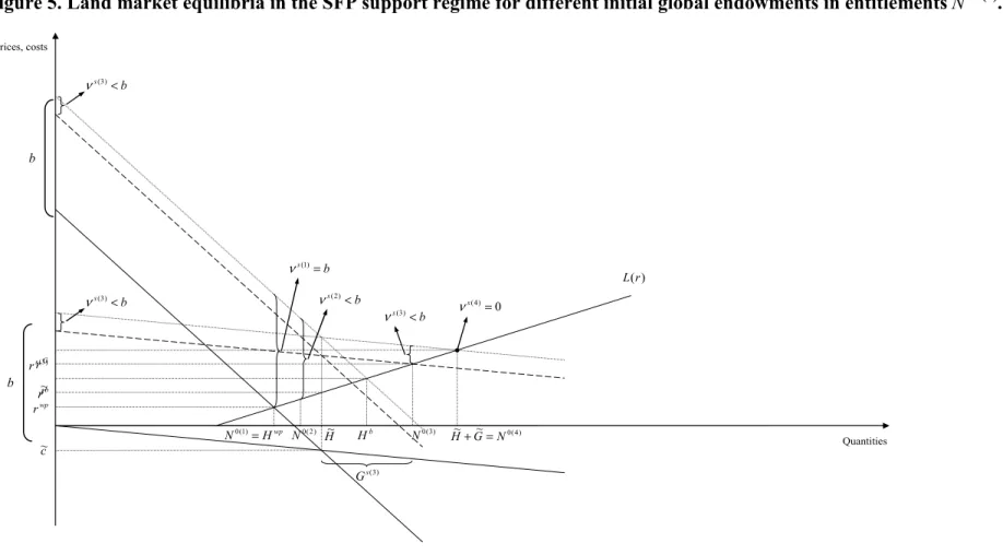
We successively consider the four regimes which are illustrated by Figure 5. The latter is drawn in the simplified case where producers 1 and 2 are assumed identical in terms of production, cost and profit structures; they can however differ in terms of initial endowments in entitlements.

Regime 1. N0 ≤Hwp =L(rwp)

In that first regime illustrated by the limit case where N0 =N0(1) =Hwpon Figure 5, the land demanded for idling under GAECs equals zero. Equilibrium conditions are defined by equations (12a) to (12e) and Proposition 2 holds. In that first regime, the SPS has no impact on individual land demands for cultivation, on total land demanded for cultivation and on the equilibrium land rental price. There are entitlement exchanges at a unit price vs =b from the over-endowed producer (if he exists) towards the under-endowed producer (if he exists).

Regime 2. Hwp ≤N0 ≤H~

In that second regime illustrated by a number of entitlements set to N0(2) on Figure 5, the land demanded for idling is still equal to zero. Equilibrium conditions are defined by equations (13a) to (13f), except that Hb should be replaced by H~, and Proposition 3 holds. In that second regime, the SPS has a positive impact on individual land demands for cultivation, on total land demand for cultivation and on the equilibrium land price (relative to the no-support regime). Payments partially capitalize in land prices: the higher the number of entitlements, the greater the capitalization in land prices. Payments also capitalize in entitlement exchange prices: the higher the number of entitlements, the lower the capitalization in entitlement prices.

Figure 5. Land market equilibria in the SFP support regime for different initial global endowments in entitlementsN0 (a). H~ c ~ r ~ wp H N0(1)= b H ~ ~ 0(4) N G H+ = ) 2 ( 0 N 0(3) N ) 3 ( s G b s(1)₌ ν b s(2)_< ν _νs(4)₌₀ b s(3)_< ν ) 3 ( s r wp r b s(3)_< ν b s(3)_< ν ) (r L Prices, costs Quantities

(a) Hwp is the total area demanded in the zero support regime, Hb is the total number of hectares that would be demanded in a policy regime where support would be granted through direct aids per hectare of unit amount b, and H~ and G~ are the numbers of hectares that would be demanded for cultivation and idling under GAECs, respectively, in a policy regime where income support is granted through direct aids per hectare of unit amount b and production is not required. b r G r b b

Regime 3. H~≤ N0 ≤H~+G~

In that third regime illustrated by a number of entitlements set to N0(3) on Figure 5, the land quantity demanded for idling under GAECs is positive. More specifically, for a number of entitlements set to N0(3), the land market equilibrium occurs at point Es(3) which corresponds to a land price of rs(3) >rs(2) >rwp and a land quantity used in the agricultural sector of

wp

H N

N0(3) > 0(2) > : among these N0(3) hectares, H~ hectares are effectively demanded for cultivation and Gs(3) =N0(3) −H~ are demanded for idling under GAECs. All entitlements are activated, and there are entitlement exchanges at a unit price vs(3) <vs(2) <b from the over-endowed farmer (if he exists) towards the under-over-endowed farmer (if he exists).

More generally, equilibrium conditions in that third regime with H~ ≤N0 ≤H~+G~ can be expressed as: b vs < ≤ 0 , (24a) i s i h h = ~ with h~_i defined by ∂

π

_i(p_i,w,h~_i,l_i)/∂h=−∂CJ_i(h~_i)/∂h=c~_i <0, (24b) H h H i i s 2 ~ ~ 1 = =

_∑

= , (24c) ) ( 0 s r L N = , (24d) ) ( )] ( ) / ) ( [( 2 1 1 s i s s i i m m b r v L r CJ ∂ + + = −∂

∑

= − _{, (24e)} b v r g g h CJ_{i i}+ _is ∂ = s + s − ∂ − (~ )/ , (24f) H N g G i s i s 2 0 ~ 1 − = =

∑

= , (24g) s i i s i h g n = ~+ , (24h) G H N n i s i ~ ~ 0 2 1 + ≤ =

∑

= . (24i)

Equation (24d) defines the equilibrium land rental price while equation (24e) defines the equilibrium entitlement rental price, once the equilibrium land price is determined. Equations (24b) and (24c) define the individual and total land demand functions for cultivation, respectively. Equation (24f) defines the individual land demand functions for idling under

GAECs and equation (24g) defines the total land demand for idling under GAECs. Finally, equations (24h) and (24i) define the individual and aggregate entitlement demand functions, respectively.

Payments capitalize in land and entitlement prices; the degree of capitalization in land prices (respectively, entitlement prices) increases (decreases) with the number of entitlements; in the upper limit case corresponding to a number of entitlements N0 set to H~+G~, capitalization in land prices is maximum while capitalization in entitlement prices is null (vs =0).

Relative to the zero support regime, one immediately notes that the SPS has a positive effect on the number of hectares in cultivation (H~ >Hwp): the SPS is not decoupled at the extensive margin of production. More interesting is the comparison of the SPS with a policy regime where support is granted through per-hectare direct aids of unit amount b assuming that production is required to benefit from these area payments. In that alternative policy regime, there is no land demanded for idling and the land demanded for cultivation is equal to _Hb_.

Recalling that we assumed here that H~<Hb, one verifies that Hb <H~+G~: Total land used in the agricultural sector is greater in the SPF policy regime relative to the regime of per-hectare direct aids, but part of the land demanded is not cultivated so that the number of hectares under cultivation is lower in the SPS relative to the policy regime of area payments.

Regime 4. H~+G~≤N0

In that fourth regime illustrated by the limit case where N0(4) =H~ +G~ on Figure 5, the number of hectares demanded for cultivation is H~, the number of hectares demanded for idling under GAECs is G~, the land equilibrium price is equal to rG (payment capitalization in land prices is maximum) and the entitlement equilibrium price is equal to zero (payment capitalization in entitlement prices is null). There is an excess of entitlements relative to the total number of hectares used in the agricultural sector: the quantity N0 −(H~+G~)≥0 of entitlements is not activated.

4. Implications and concluding remarks

The main conclusion that can be drawn from the analysis developed in the previous section is that the very nature of the new CAP SFP scheme adopted in the EU in 2003 crucially depends on the total number of entitlements which are initially made available. Two situations have to be distinguished depending on the relative positions of (i) the aggregate marginal profit function, (ii) the aggregate marginal cost function of maintaining non-cultivated land in GAECs and (iii) the aggregate marginal land supply function. These two cases are illustrated in the two panels of Figure 6 which helps summarising and interpreting our findings.

The first case (panel a of Figure 6) corresponds to the situation where the number of hectares that would be demanded for cultivation in a policy regime where the support is granted through direct aids per hectare of unit amount b and production is not required is greater than the number of hectares that would be demanded in the same policy regime but production is required (case where H~ ≥Hb). Then:

- when the initial number of entitlements is lower than or equal to the number of hectares that would be demanded by farmers for cultivation in a regime where no support is granted (N0 ≤Hwp), SFP entitlements work as lump-sum transfers which only have the effect of raising farmers’ income: relative to the zero support regime, neither do they modify the amount of land that is demanded, nor do they capitalize into the land rental price.

- when the initial number of entitlements is greater than or equal to the number of hectares that would be demanded by farmers for cultivation in a zero support regime and lower than or equal to the number of hectares that would be demanded for cultivation in a policy regime where the support is granted through direct aids per hectare of unit amount b

and production is required (Hwp ≤N0 ≤Hb), SFP entitlements work as direct aids per hectare that would be granted on a binding base area (defined as _N0 _{hectares): the total land}

demanded for production increases to the base area N0 and the land rental price raises as part of the support granted through SFP entitlements capitalize into it.

- eventually, when the initial number of entitlements is greater than or equal to the number of hectares that would be demanded by farmers for cultivation in a policy regime where the support is granted through direct aids per hectare of unit amount b and production is required (Hb ≤ N0), SFP entitlements work just as unlimited direct aids per hectare: the total land demanded for production is Hb, the capitalization of support into the land rental

price is complete, and the base-area-equivalent N0 is no longer binding so that a quantity of

b

H

N0 − entitlements is not activated.

The second case (panel b of Figure 6) takes place when the number of hectares that would be demanded for cultivation in a policy regime where the support is granted through direct aids per hectare of unit amount b and production is not required is lower than the number of hectares that would be demanded in the same policy regime but production is required (case where H~ ≤Hb). Then:

- when the initial number of entitlements is lower than or equal to the number of hectares that would be demanded by farmers for cultivation in a regime where no support is granted (N0 ≤Hwp), SFP entitlements work as lump-sum transfers.

- when the initial number of entitlements is greater than or equal to the number of hectares that would be demanded by farmers for cultivation in a zero support regime and lower than or equal to the number of hectares that would be demanded for cultivation in a policy regime where the support is granted through direct aids per hectare of unit amount b

and production is not required (Hwp ≤N0 ≤H~), SFP entitlements work as direct aids per hectare that would be granted on a binding base-area-equivalent of N0 hectares.

- when the initial number of entitlements is greater than or equal to the number of hectares demanded for cultivation and lower than or equal to the total number of hectares demanded (for cultivation or idling) in a policy regime where the support is granted through direct aids per hectare of unit amount b and production is not required (H~ ≤N0 ≤H~+G~), SFP entitlements have three effects: first, they induce an aggregate land demand for cultivation of H~ which is greater than the demand that would occur in the zero support regime (Hwp ≤ H~), but to a lesser extent than direct aids per hectare would (H~ ≤Hb); second, the total land demanded is constrained by the base-area-equivalent N0 and part of this land (N0 −H~) is idled; third, the land rental price is raised relative to the zero support regime.