Chapter 6
INTERVALS Statement
Chapter Table of Contents
OVERVIEW . . . 217
GETTING STARTED . . . 218
Computing Statistical Intervals . . . 218
Computing One-Sided Lower Prediction Limits . . . 220
SYNTAX . . . 222
Summary of Options . . . 222
Dictionary of Options . . . 223
DETAILS . . . 225
Methods for Computing Statistical Intervals . . . 225
OUTINTERVALS= Data Set . . . 228
Chapter 6
INTERVALS Statement
Overview
The INTERVALS statement tabulates various statistical intervals for selected process variables. The types of intervals you can request include
approximate simultaneous prediction intervals for future observations prediction intervals for the mean of future observations
approximate statistical tolerance intervals that contain at least a specified pro-portion of the population
confidence intervals for the population mean
prediction intervals for the standard deviation of future observations confidence intervals for the population standard deviation
These intervals are computed assuming the data are sampled from a normal popula-tion. See Hahn and Meeker (1991) for a detailed discussion of these intervals. You can use options in the INTERVALS statement to
specify which intervals to compute
provide probability or confidence levels for intervals suppress printing of output tables
create an output data set containing interval information
Getting Started
This section introduces the INTERVALS statement with simple examples that illus-trate commonly used options. Complete syntax for the INTERVALS statement is presented in the “Syntax” section on page 222.
Computing Statistical Intervals
The following statements create the data set CANS, which contains measurements See CAPINT1
in the SAS/QC
Sample Library (in ounces) of the fluid weights of 100 drink cans. The filling process is assumed to be in statistical control.
data cans;
label weight = ’Fluid Weight (ounces)’; input weight @@; datalines; 12.07 12.02 12.00 12.01 11.98 11.96 12.04 12.05 12.01 11.97 12.03 12.03 12.00 12.04 11.96 12.02 12.06 12.00 12.02 11.91 12.05 11.98 11.91 12.01 12.06 12.02 12.05 11.90 12.07 11.98 12.02 12.11 12.00 11.99 11.95 11.98 12.05 12.00 12.10 12.04 12.06 12.04 11.99 12.06 11.99 12.07 11.96 11.97 12.00 11.97 12.09 11.99 11.95 11.99 11.99 11.96 11.94 12.03 12.09 12.03 11.99 12.00 12.05 12.04 12.05 12.01 11.97 11.93 12.00 11.97 12.13 12.07 12.00 11.96 11.99 11.97 12.05 11.94 11.99 12.02 11.95 11.99 11.91 12.06 12.03 12.06 12.05 12.04 12.03 11.98 12.05 12.05 12.11 11.96 12.00 11.96 11.96 12.00 12.01 11.98 ;
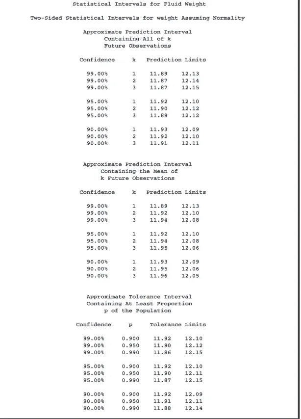
Note that this data set is introduced in “Computing Descriptive Statistics” on page 9 of Chapter 1, “PROC CAPABILITY and General Statements.” The analysis in that section provides evidence that the weight measurements are normally distributed. By default, the INTERVALS statement computes and prints the six intervals de-scribed in the entry for the METHODS= option on page 223. The following state-ments tabulate these intervals for the variable WEIGHT:
title ’Statistical Intervals for Fluid Weight’; proc capability data=cans noprint;
intervals weight; run;
Chapter 6. Getting Started
Statistical Intervals for Fluid Weight
Two-Sided Statistical Intervals for weight Assuming Normality
Approximate Prediction Interval Containing All of k Future Observations
Confidence k Prediction Limits
99.00% 1 11.89 12.13 99.00% 2 11.87 12.14 99.00% 3 11.87 12.15 95.00% 1 11.92 12.10 95.00% 2 11.90 12.12 95.00% 3 11.89 12.12 90.00% 1 11.93 12.09 90.00% 2 11.92 12.10 90.00% 3 11.91 12.11
Approximate Prediction Interval Containing the Mean of k Future Observations
Confidence k Prediction Limits
99.00% 1 11.89 12.13 99.00% 2 11.92 12.10 99.00% 3 11.94 12.08 95.00% 1 11.92 12.10 95.00% 2 11.94 12.08 95.00% 3 11.95 12.06 90.00% 1 11.93 12.09 90.00% 2 11.95 12.06 90.00% 3 11.96 12.05
Approximate Tolerance Interval Containing At Least Proportion
p of the Population
Confidence p Tolerance Limits
99.00% 0.900 11.92 12.10 99.00% 0.950 11.90 12.12 99.00% 0.990 11.86 12.15 95.00% 0.900 11.92 12.10 95.00% 0.950 11.90 12.11 95.00% 0.990 11.87 12.15 90.00% 0.900 11.92 12.09 90.00% 0.950 11.91 12.11 90.00% 0.990 11.88 12.14
Two-Sided Statistical Intervals for weight Assuming Normality
Confidence Limits Containing the Mean
Confidence Confidence Limits
99.00% 11.997 12.022
95.00% 12.000 12.019
90.00% 12.002 12.017
Prediction Interval Containing the Standard Deviation of
k Future Observations
Confidence k Prediction Limits
99.00% 2 0.0003 0.1348 99.00% 3 0.0033 0.1110 95.00% 2 0.0015 0.1069 95.00% 3 0.0075 0.0919 90.00% 2 0.0030 0.0932 90.00% 3 0.0106 0.0825
Confidence Limits Containing the Standard Deviation
Confidence Confidence Limits
99.00% 0.040 0.057
95.00% 0.041 0.055
90.00% 0.042 0.053
Figure 6.2. Statistical Intervals for WEIGHT(continued from page 219)
Computing One-Sided Lower Prediction Limits
You can specify options after the slash (/) in the INTERVALS statement to control See CAPINT1
in the SAS/QC
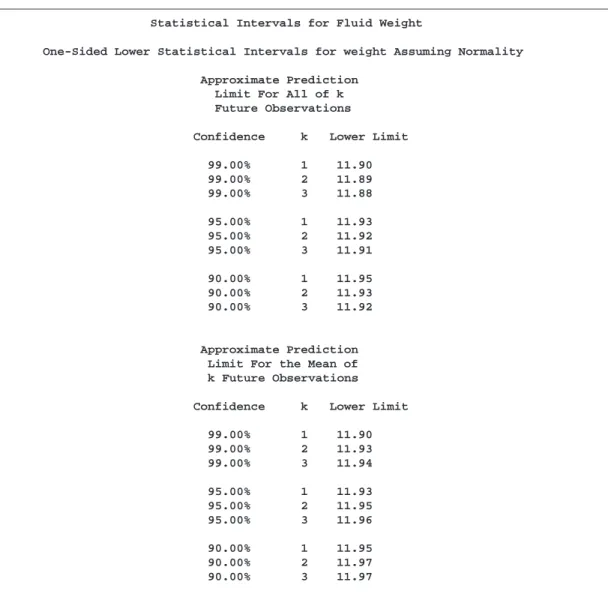
Sample Library the computation and printing of intervals. The following statements produce a table of one-sided lower prediction limits for the mean, which is displayed in Figure 6.3:
title ’Statistical Intervals for Fluid Weight’; proc capability data=cans noprint;
intervals weight / methods = 1 2 type = lower; run;
The METHODS= option specifies which intervals to compute, and the TYPE= op-tion requests one-sided lower limits. All the opop-tions available in the INTERVALS statement are listed in “Summary of Options” on page 222 and are described in “Dic-tionary of Options” on page 223.
Chapter 6. Getting Started
Statistical Intervals for Fluid Weight
One-Sided Lower Statistical Intervals for weight Assuming Normality
Approximate Prediction Limit For All of k Future Observations
Confidence k Lower Limit
99.00% 1 11.90 99.00% 2 11.89 99.00% 3 11.88 95.00% 1 11.93 95.00% 2 11.92 95.00% 3 11.91 90.00% 1 11.95 90.00% 2 11.93 90.00% 3 11.92 Approximate Prediction Limit For the Mean of k Future Observations
Confidence k Lower Limit
99.00% 1 11.90 99.00% 2 11.93 99.00% 3 11.94 95.00% 1 11.93 95.00% 2 11.95 95.00% 3 11.96 90.00% 1 11.95 90.00% 2 11.97 90.00% 3 11.97
Syntax
The syntax for the INTERVALS statement is as follows: INTERVALS<variables></options>;
You can specify INTERVAL as an alias for INTERVALS. You can use any number of INTERVALS statements in the CAPABILITY procedure. The components of the INTERVALS statement are described as follows.
variables
gives a list of variables for which to compute intervals. If you specify a VAR state-ment, the variables must also be listed in the VAR statement. Otherwise, the variables can be any numeric variable in the input data set. If you do not specify a list of
vari-ables, then by default the INTERVALS statement computes intervals for all variables
in the VAR statement (or all numeric variables in the input data set if you do not use a VAR statement).
options
alter the defaults for computing and printing intervals and for creating output data sets.
Summary of Options
The following tables list the INTERVALS statement options by function. For com-plete descriptions, see “Dictionary of Options” on page 223.
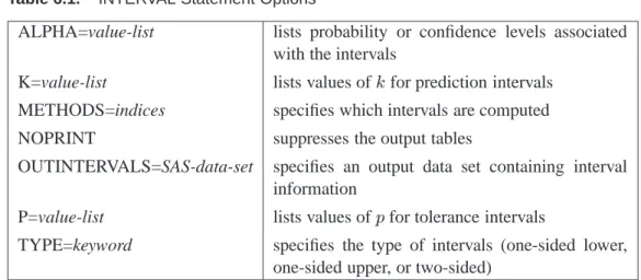
Table 6.1. INTERVAL Statement Options
ALPHA=value-list lists probability or confidence levels associated with the intervals
K=value-list lists values ofkfor prediction intervals METHODS=indices specifies which intervals are computed NOPRINT suppresses the output tables
OUTINTERVALS=SAS-data-set specifies an output data set containing interval information
P=value-list lists values ofpfor tolerance intervals
TYPE=keyword specifies the type of intervals (one-sided lower, one-sided upper, or two-sided)
Chapter 6. Syntax
Dictionary of Options
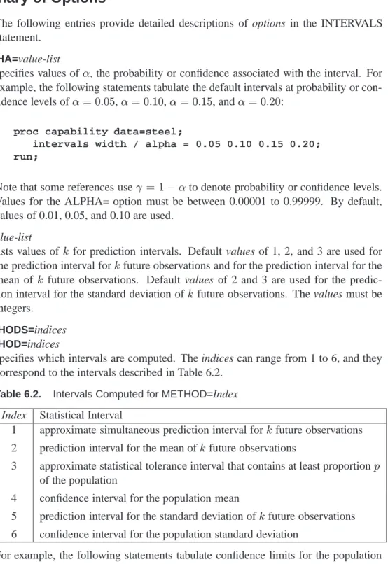
The following entries provide detailed descriptions of options in the INTERVALS statement.
ALPHA=value-list
specifies values of, the probability or confidence associated with the interval. For example, the following statements tabulate the default intervals at probability or con-fidence levels of=0:05,=0:10,=0:15, and=0:20:
proc capability data=steel;
intervals width / alpha = 0.05 0.10 0.15 0.20; run;
Note that some references use =1,to denote probability or confidence levels. Values for the ALPHA= option must be between 0.00001 to 0.99999. By default, values of 0.01, 0.05, and 0.10 are used.
K=value-list
lists values ofk for prediction intervals. Default values of 1, 2, and 3 are used for the prediction interval forkfuture observations and for the prediction interval for the mean ofk future observations. Default values of 2 and 3 are used for the predic-tion interval for the standard deviapredic-tion ofk future observations. The values must be integers.
METHODS=indices
METHOD=indices
specifies which intervals are computed. The indices can range from 1 to 6, and they correspond to the intervals described in Table 6.2.
Table 6.2. Intervals Computed for METHOD=Index Index Statistical Interval
1 approximate simultaneous prediction interval forkfuture observations 2 prediction interval for the mean ofkfuture observations
3 approximate statistical tolerance interval that contains at least proportionp of the population
4 confidence interval for the population mean
5 prediction interval for the standard deviation ofkfuture observations 6 confidence interval for the population standard deviation
For example, the following statements tabulate confidence limits for the population mean (METHOD=4) and confidence limits for the population standard deviation (METHOD=6):
proc capability data=steel;
intervals width / methods=4 6; run;
Formulas for the intervals are given in “Methods for Computing Statistical Intervals” on page 225. By default, the procedure computes all six intervals.
NOPRINT
suppresses the tables produced by default. This option is useful when you only want to save the interval information in an OUTINTERVALS= data set.
OUTINTERVALS=SAS-data-set
OUTINTERVAL=SAS-data-set
OUTINT=SAS-data-set
specifies an output SAS data set containing the intervals and related information. For example, the following statements create a data set named INTS containing intervals for the variable WIDTH:
proc capability data=steel;
intervals width / outintervals=ints; run;
See “OUTINTERVALS= Data Set” on page 228 for details. P=value-list
lists values of p for the tolerance intervals. These values must be between 0.00001 to 0.99999. Note that the P= option applies only to the tolerance intervals (METHODS=3). By default, values of 0.90, 0.95, and 0.99 are used.
TYPE=LOWER | UPPER | TWOSIDED
determines whether the intervals computed are one-sided lower, one-sided upper, or two-sided intervals, respectively. See “Computing One-Sided Lower Prediction Limits” on page 220 for an example. The default interval type is TWOSIDED.
Chapter 6. Details
Details
This section provides details on the following topics:
formulas for statistical intervals OUTINTERVALS= data sets
Methods for Computing Statistical Intervals
The formulas for statistical intervals given in this section use the following notation: Notation Definition
n number of nonmissing values for a variable
X mean of variable
s standard deviation of variable z
100
thpercentile of the standard normal distribution
t
() 100
thpercentile of the central
tdistribution withdegrees of freedom t
0
(;) 100
thpercentile of the noncentral
tdistribution with noncentrality parameteranddegrees of freedom
F ( 1 ; 2 ) 100
thpercentile of the F distribution with
1 degrees of freedom in the numerator and
2degrees of freedom in the denominator 2 () 100 thpercentile of the 2
distribution withdegrees of freedom. The values of the variable are assumed to be independent and normally distributed. The intervals are computed using the degrees of freedom as the divisor for the stan-dard deviation s. This divisor corresponds to the default of VARDEF=DF in the PROC CAPABILITY statement. If you specify another value for the VARDEF= op-tion, intervals are not computed.
You select the intervals to be computed with the METHODS= option. The next six sections give computational details for each of the METHODS= options.
METHODS=1
This requests an approximate simultaneous prediction interval fork future observa-tions. Two-sided intervals are computed using the conservative approximations
Lower Limit = X,t 1, 2k (n,1)s q 1+ 1 n Upper Limit = X+t 1, 2k (n,1)s q 1+ 1 n
One-sided limits are computed using the conservative approximation Lower Limit = X,t 1, k (n,1)s q 1+ 1 n Upper Limit = X+t 1, k (n,1)s q 1+ 1 n
Hahn (1970c) states that these approximations are satisfactory except for combina-tions of smalln, largek, and large. Refer also to Hahn (1969 and 1970a) and Hahn and Meeker (1991).
METHODS=2
This requests a prediction interval for the mean ofk future observations. Two-sided intervals are computed as
Lower Limit = X,t 1, 2 (n,1)s q 1 k + 1 n Upper Limit = X+t 1, 2 (n,1)s q 1 k + 1 n One-sided limits are computed as
Lower Limit = X,t 1, (n,1)s q 1 k + 1 n Upper Limit = X+t 1, (n,1)s q 1 k + 1 n METHODS=3
This requests an approximate statistical tolerance interval that contains at least pro-portionpof the population. Two-sided intervals are approximated by
Lower Limit = X,g(p;n;1,)s Upper Limit = X+g(p;n;1,)s whereg(p;n;1,)=z1+p 2 (1+ 1 2n ) q n,1 2 (n,1) . Exact one-sided limits are computed as
Lower Limit = X,g 0 (p;n;1,)s Upper Limit = X+g 0 (p;n;1,)s whereg 0 (p;n;1,)= 1 p n t 0 1, (z p p n;n,1).
Chapter 6. Details
In some cases (for example, ifz p p nis large),g 0 (p;n;1,)is approximated by 1 a z p + q z 2 p ,ab wherea=1, z 2 1, 2(n,1) andb=z 2 p , z 2 1, n .
Hahn (1970b) states that this approximation is “poor for very smalln, especially for largepand large1,, and is not advised forn<8.” Refer also to Hahn and Meeker (1991).
METHODS=4
This requests a confidence interval for the population mean. Two-sided intervals are computed as Lower Limit = X,t 1, 2 (n,1) s p n Upper Limit = X+t 1, 2 (n,1) s p n One-sided limits are computed as
Lower Limit = X,t 1, (n,1) s p n Upper Limit = X+t 1, (n,1) s p n METHODS=5
This requests a prediction interval for the standard deviation ofkfuture observations. Two-sided intervals are computed as
Lower Limit = s F 1, 2 (n,1;k,1) , 1 2 Upper Limit = s F 1, 2 (k,1;n,1) 1 2
One-sided limits are computed as Lower Limit = s(F 1, (n,1;k,1)) , 1 2 Upper Limit = s(F 1, (k,1;n,1)) 1 2 METHODS=6
This requests a confidence interval for the population standard deviation. Two-sided intervals are computed as
Lower Limit = s r n,1 2 1, 2 (n,1) Upper Limit r n,1
One-sided limits are computed as Lower Limit = s q n,1 2 1, (n,1) Upper Limit = s q n,1 2 (n,1)
OUTINTERVALS= Data Set
Each INTERVALS statement can create an output data set specified with the OUT-INTERVALS= option. The OUTOUT-INTERVALS= data set contains statistical intervals and related parameters.
The number of observations in the OUTINTERVALS= data set depends on the num-ber of variables analyzed, the numnum-ber of tests specified, and the results of the tests. The OUTINTERVALS= data set is constructed as follows:
The OUTINTERVALS= data set contains a group of observations for each vari-able analyzed.
Each group contains one or more observations for each interval you specify with the METHODS= option. The actual number depends upon the number of combinations of the ALPHA=, K=, and P= values.
The following variables are saved in the OUTINTERVALS= data set: Variable Description
– ALPHA– value ofassociated with the intervals – K– value of K= for the prediction intervals – LOWER– lower endpoint of interval
– METHOD– interval index(16)
– P– value of P= for the tolerance intervals
– TYPE– type of interval (ONESIDED or TWOSIDED) – UPPER– upper endpoint of interval
– VAR– variable name
If you use a BY statement, the BY variables are also saved in the OUTINTERVALS= data set.
Chapter 6. Details
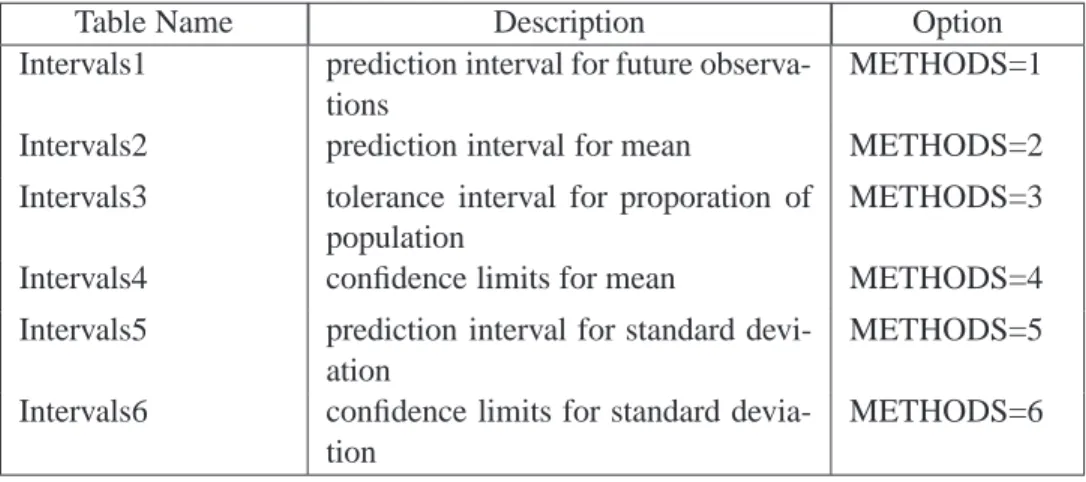
ODS Tables
The following table summarizes the ODS tables that you can request with the IN-TERVALS statement.
Table 6.3. ODS Tables Produced with the INTERVALS Statement
Table Name Description Option
Intervals1 prediction interval for future observa-tions
METHODS=1 Intervals2 prediction interval for mean METHODS=2 Intervals3 tolerance interval for proporation of
population
METHODS=3 Intervals4 confidence limits for mean METHODS=4 Intervals5 prediction interval for standard
devi-ation
METHODS=5 Intervals6 confidence limits for standard
devia-tion
SAS/QC User’s Guide, Version 8
Copyright © 1999 SAS Institute Inc., Cary, NC, USA. ISBN 1–58025–493–4
All rights reserved. Printed in the United States of America. No part of this publication may be reproduced, stored in a retrieval system, or transmitted, by any form or by any means, electronic, mechanical, photocopying, or otherwise, without the prior written permission of the publisher, SAS Institute Inc.
U.S. Government Restricted Rights Notice. Use, duplication, or disclosure of the
software by the government is subject to restrictions as set forth in FAR 52.227–19 Commercial Computer Software-Restricted Rights (June 1987).
SAS Institute Inc., SAS Campus Drive, Cary, North Carolina 27513. 1st printing, October 1999
SAS®and all other SAS Institute Inc. product or service names are registered trademarks
or trademarks of SAS Institute in the USA and other countries.®indicates USA
registration.
IBM®, ACF/VTAM®, AIX®, APPN®, MVS/ESA®, OS/2®, OS/390®, VM/ESA®, and VTAM®
are registered trademarks or trademarks of International Business Machines Corporation.