HAL Id: hal-02355101
https://hal.archives-ouvertes.fr/hal-02355101
Submitted on 8 Nov 2019
HAL
is a multi-disciplinary open access
archive for the deposit and dissemination of
sci-entific research documents, whether they are
pub-lished or not. The documents may come from
teaching and research institutions in France or
abroad, or from public or private research centers.
L’archive ouverte pluridisciplinaire
HAL
, est
destinée au dépôt et à la diffusion de documents
scientifiques de niveau recherche, publiés ou non,
émanant des établissements d’enseignement et de
recherche français ou étrangers, des laboratoires
publics ou privés.
LDAS-Monde Sequential Assimilation of Satellite
Derived Observations Applied to the Contiguous US: An
ERA-5 Driven Reanalysis of the Land Surface Variables
Clément Albergel, Simon Munier, Aymeric Bocher, Bertrand Bonan, Yongjun
Zheng, Clara Draper, Delphine Leroux, Jean-Christophe Calvet
To cite this version:
Clément Albergel, Simon Munier, Aymeric Bocher, Bertrand Bonan, Yongjun Zheng, et al..
LDAS-Monde Sequential Assimilation of Satellite Derived Observations Applied to the Contiguous US: An
ERA-5 Driven Reanalysis of the Land Surface Variables. Remote Sensing, MDPI, 2018, 10 (10),
pp.1627. �10.3390/rs10101627�. �hal-02355101�
remote sensing
ArticleLDAS-Monde Sequential Assimilation of Satellite
Derived Observations Applied to the Contiguous US:
An ERA-5 Driven Reanalysis of the Land
Surface Variables
Clement Albergel1,* , Simon Munier1 , Aymeric Bocher1, Bertrand Bonan1, Yongjun Zheng1, Clara Draper2, Delphine J. Leroux1and Jean-Christophe Calvet1
1 CNRM UMR 3589, Météo-France/CNRS, 31057 Toulouse, France; [email protected] (S.M.);
[email protected] (A.B.); [email protected] (B.B.); [email protected] (Y.Z.); [email protected] (D.J.L.); [email protected] (J.-C.C.)
2 CIRES/NOAA Earth System Research Laboratory, Boulder, CO 80309, USA; [email protected]
* Correspondence: [email protected]
Received: 5 September 2018; Accepted: 10 October 2018; Published: 12 October 2018
Abstract:Land data assimilation system (LDAS)-Monde, an offline land data assimilation system with global capacity, is applied over the CONtiguous US (CONUS) domain to enhance monitoring accuracy for water and energy states and fluxes. LDAS-Monde ingests satellite-derived surface soil moisture (SSM) and leaf area index (LAI) estimates to constrain the interactions between soil, biosphere, and atmosphere (ISBA) land surface model (LSM) coupled with the CNRM (Centre National de Recherches Météorologiques) version of the total runoff integrating pathways (CTRIP) continental hydrological system (ISBA-CTRIP). LDAS-Monde is forced by the ERA-5 atmospheric reanalysis from the European Center for Medium Range Weather Forecast (ECMWF) from 2010 to 2016 leading to a seven-year, quarter degree spatial resolution offline reanalysis of land surface variables (LSVs) over CONUS. The impact of assimilating LAI and SSM into LDAS-Monde is assessed over North America, by comparison to satellite-driven model estimates of land evapotranspiration from the Global Land Evaporation Amsterdam Model (GLEAM) project, and upscaled ground-based observations of gross primary productivity from the FLUXCOM project. Taking advantage of the relatively dense data networks over CONUS, we have also evaluated the impact of the assimilation against in situ measurements of soil moisture from the USCRN (US Climate Reference Network), together with river discharges from the United States Geological Survey (USGS) and the Global Runoff Data Centre (GRDC). Those data sets highlight the added value of assimilating satellite derived observations compared with an open-loop simulation (i.e., no assimilation). It is shown that LDAS-Monde has the ability not only to monitor land surface variables but also to forecast them, by providing improved initial conditions, which impacts persist through time. LDAS-Monde reanalysis also has the potential to be used to monitor extreme events like agricultural drought. Finally, limitations related to LDAS-Monde and current satellite-derived observations are exposed as well as several insights on how to use alternative datasets to analyze soil moisture and vegetation state. Keywords:land surface modeling; data assimilation; remote sensing
1. Introduction
One of the major scientific challenges in relation to the adaptation to climate change is observing and simulating the response of land biophysical variables to extreme events, making land surface models (LSMs) constrained by high-quality gridded atmospheric variables and coupled
Remote Sens.2018,10, 1627 2 of 24
with river-routing models key tools to address these challenges [1,2]. The modelling of terrestrial variables can be improved through the dynamical integration of observations. Remote sensing observations are particularly useful in this context because of their global coverage and higher spatial resolution (10 km and below). The current fleet of Earth observation missions holds an unprecedented potential to quantify land surface variables (LSVs) [3] and many satellite-derived products relevant to the hydrological and vegetation cycles are already available at high spatial resolutions. However, satellite remote sensing observations exhibit spatial and temporal gaps and not all key LSVs can be observed. LSMs are able to provide LSV estimates at all times and locations using physically-based equations, but as remotely sensed observations, they are affected by uncertainties (e.g., parametrization representation, atmospheric forcing, initialisation). Through a weighted combination of both, LSVs can be better estimated than by either source of information alone [4]; data assimilation techniques enable one to spatially and temporally integrate observed information into LSMs in a consistent way to unobserved locations, time steps, and variables.
In the past recent years, several land data assimilation system (LDAS) have emerged at different spatial scales: “site level”, like the data assimilation system for LSMs using CLM4.5 (Community Land Model 4.5, [5]); regional, like the coupled land vegetation LDAS (CLVLDAS, [6,7]) and the famine early warning systems network (FEWSNET) LDAS (FLDAS, [8]); continental, like the North American LDAS (NLDAS, [9,10]) and the National Climate Assessment LDAS (NCA-LDAS [11]); as well as at global scale, like the global land data assimilation (GLDAS, [12]) and, more recently, LDAS-Monde [13]. LDAS-Monde has been developed to constrain the CO2-responsive version of
the ISBA (interactions between soil, biosphere, and atmosphere) LSM [14–17] using satellite derived observations within the open-source SURFEX modelling platform (SURFace Externalisee, [18]) of Meteo-France. LDAS-Monde has been implemented in a monitoring chain of terrestrial water and carbon fluxes. Unlike most of the above mentioned LDAS, LDAS-Monde is able to jointly and sequentially assimilate vegetation products such as leaf area index (LAI) together with surface soil moisture (SSM) observations [13,19–21]. Ref. [13] tested LDAS-Monde over Europe and the Mediterranean basin for the 2000–2012 period. A long term, global scale, multi-sensor satellite-derived surface soil moisture dataset (ESA CCI SSM, [22–25]) along with satellite derived LAI (GEOV1,
http://land.copernicus.eu/global/last access, June 2018), were jointly assimilated. LDAS-Monde was forced by WFDEI (WATCH-forcing-data-ERA-interim) observations based atmospheric forcing dataset [26,27] at half degree spatial resolution. Analysis impact was successfully carried out using (i) agricultural statistics over France; (ii) river discharge observations; (iii) satellite-derived estimates of land evapotranspiration from the global land evaporation amsterdam model (GLEAM) project; and (iv) spatially gridded observations-based estimates of up-scaled gross primary production and evapotranspiration from the FLUXNET network [13].
In this study, LDAS-Monde is applied and tested in a data-rich area: the CONtiguous US (CONUS, defined here as longitudes from 130.0◦W to 60.0◦W, latitudes from 20.0◦N to 55.0◦N, as shown in Figure1). LDAS-Monde is forced by the latest ERA-5 atmospheric reanalysis from the European Center for Medium Range Weather Forecast (ECMWF) from 2010 to 2016 leading to a seven-year, quarter degree spatial resolution offline reanalysis of the land surface variables (LSVs). Ref. [28] assessed ERA-5 ability to force the ISBA LSM by comparison to satellite-derived products and in situ observations covering a substantial part of the land surface storage and fluxes. They found that using ERA-5 in place of its predecessor, ERA-Interim, led to significant improvements in the representation of the LSVs linked to the terrestrial water cycle (surface soil moisture, river discharges, snow depth, and turbulent atmospheric fluxes), but did not improve the LSVs linked to the vegetation cycle (evapotranspiration, carbon uptake, and LAI). In that respect, the assimilation of LAI through ERA-5 driven reanalysis from LDAS-Monde is expected to bring clear improvements [13]. In this study, the impact of LDAS-Monde analysis with respect to an open-loop (i.e., model run without assimilation) is assessed using satellite-driven model estimates of land evapotranspiration from the Global Land Evaporation Amsterdam Model (GLEAM) project and upscaled ground-based observations of gross
Remote Sens.2018,10, 1627 3 of 24
primary productivity from the FLUXCOM project, together with river discharges from the United States Geophysical Survey (USGS) and the Global Runoff Data Centre (GRDC). Over CONUS, in situ measurements of soil moisture from the USCRN network (US Climate Reference Network) are also used in the evaluation. Section2describes the different components of LDAS-Monde as well as the evaluation data sets and strategy. Section3provides a set of statistical diagnostics to assess and evaluate the impact of the assimilation. Finally, Section4provides perspectives and future research directions.
Remote Sens. 2018, 10, x FOR PEER REVIEW 3 of 24 (i.e., model run without assimilation) is assessed using satellite-driven model estimates of land evapotranspiration from the Global Land Evaporation Amsterdam Model (GLEAM) project and upscaled ground-based observations of gross primary productivity from the FLUXCOM project, together with river discharges from the United States Geophysical Survey (USGS) and the Global Runoff Data Centre (GRDC). Over CONUS, in situ measurements of soil moisture from the USCRN network (US Climate Reference Network) are also used in the evaluation. Section 2 describes the different components of LDAS-Monde as well as the evaluation data sets and strategy. Section 3 provides a set of statistical diagnostics to assess and evaluate the impact of the assimilation. Finally, Section 4 provides perspectives and future research directions.
(a) (b)
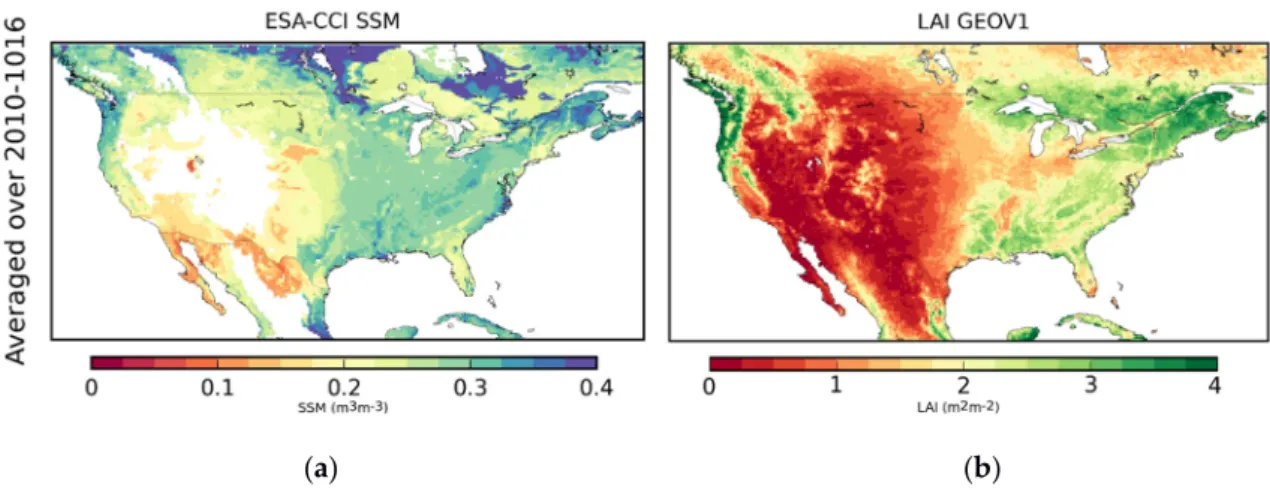
Figure 1. Averaged (a) surface soil moisture from the Climate Change Initiative project of ESA (for pixels with less than 15% of urban areas and with an elevation of less than 1500 m above sea level); (b) GEOV1 leaf area index from the Copernicus Global Land Service project (for pixels covered by more than 90% of vegetation) from 2010 to 2016. ESA CCI SSM—European Space Agency and Climate Change Initiative surface soil moisture; LAI—leaf area index.
2. Data and Methods
2.1. LDAS-Monde System Components
LDAS-Monde allows sequential assimilation of satellite derived land observations at a global scale. The assimilation is performed into the open-access SURFEX modelling platform of Météo-France (SURFace Externalisée, [18]). It produces offline re-analyses of LSVs using (i) an LSM along with data assimilation techniques, (ii) observations, and (iii) atmospheric forcing. Those components of LDAS-Monde are briefly described below.
2.1.1. The SURFEX Modelling Platform
LDAS-Monde uses the CO2-responsive version of ISBA embedded within the SURFEX
platform. The most recent version of SURFEX (version 8.1) is used in this study with the “NIT” plant biomass monitoring option for ISBA. In this configuration, ISBA simulates leaf-scale physiological processes and plant growth [15–17]. The dynamic evolution of the vegetation biomass and LAI variables is driven by photosynthesis in response to atmospheric and climate conditions. Photosynthesis enables vegetation growth resulting from the CO2 uptake. During the growing
phase, enhanced photosynthesis corresponds to a CO2 uptake, which results in vegetation growth
from the LAI minimum threshold (prescribed as 1 m2 m−2 for coniferous forest or 0.3 m2 m−2 for
other vegetation types). Transfers of water and heat through the soil rely on a multilayer diffusion scheme [29,30]. The ISBA parameters are defined for 12 generic land surface patches. They include nine plant functional types (needle leaf trees, evergreen broadleaf trees, deciduous broadleaf trees, C3 crops, C4 crops, C4 irrigated crops, herbaceous, tropical herbaceous, and wetlands) as well as bare soil, rocks, and permanent snow and ice surfaces.
Figure 1. Averaged (a) surface soil moisture from the Climate Change Initiative project of ESA (for pixels with less than 15% of urban areas and with an elevation of less than 1500 m above sea level); (b) GEOV1 leaf area index from the Copernicus Global Land Service project (for pixels covered by more than 90% of vegetation) from 2010 to 2016. ESA CCI SSM—European Space Agency and Climate Change Initiative surface soil moisture; LAI—leaf area index.
2. Data and Methods
2.1. LDAS-Monde System Components
LDAS-Monde allows sequential assimilation of satellite derived land observations at a global scale. The assimilation is performed into the open-access SURFEX modelling platform of Météo-France (SURFace Externalisée, [18]). It produces offline re-analyses of LSVs using (i) an LSM along with data assimilation techniques, (ii) observations, and (iii) atmospheric forcing. Those components of LDAS-Monde are briefly described below.
2.1.1. The SURFEX Modelling Platform
LDAS-Monde uses the CO2-responsive version of ISBA embedded within the SURFEX platform.
The most recent version of SURFEX (version 8.1) is used in this study with the “NIT” plant biomass monitoring option for ISBA. In this configuration, ISBA simulates leaf-scale physiological processes and plant growth [15–17]. The dynamic evolution of the vegetation biomass and LAI variables is driven by photosynthesis in response to atmospheric and climate conditions. Photosynthesis enables vegetation growth resulting from the CO2uptake. During the growing phase, enhanced photosynthesis
corresponds to a CO2uptake, which results in vegetation growth from the LAI minimum threshold
(prescribed as 1 m2m−2for coniferous forest or 0.3 m2m−2for other vegetation types). Transfers of
water and heat through the soil rely on a multilayer diffusion scheme [29,30]. The ISBA parameters are defined for 12 generic land surface patches. They include nine plant functional types (needle leaf trees, evergreen broadleaf trees, deciduous broadleaf trees, C3 crops, C4 crops, C4 irrigated crops, herbaceous, tropical herbaceous, and wetlands) as well as bare soil, rocks, and permanent snow and ice surfaces.
This version of ISBA is coupled to the CTRIP river routing model through OASIS-MCT [31] in order to simulate streamflows of the main rivers [32–35]. Besides, a single-source energy budget of a
Remote Sens.2018,10, 1627 4 of 24
soil/vegetation composite is computed. SURFEX also involves data assimilation techniques to analyse LSVs from the ISBA LSM.
This study makes use of the simplified version of an extended Kalman filter (SEKF), as already used and described in [13,19,21,36]. The SEKF uses finite differences from perturbed simulations to estimate the linear tangent model linking the model state control variables to the observed variables. Satellite derived surface soil moisture (SSM) and leaf area index (LAI) are simultaneously assimilated to update eight model state control variables (i.e., control variables); LAI and soil moisture from seven layers of soil, from 1 cm to 100 cm. Assimilating SSM and LAI within LDAS-Monde results in updates of the LSM variables in different ways. Model variables corresponding to the observations are first updated through the Kalman gain computed by the SEKF. Secondly, control variables are updated through their sensitivity to the observed variables. For example, the assimilation of LAI impacts LAI itself, but also soil moisture from the seven layers present in the state vector and the assimilation of SSM impacts LAI. Finally, other variables are indirectly modified by the analysis through biophysical processes and feedbacks in the model by updates of the control variables.
2.1.2. ESA CCI Surface Soil Moisture and CGLS Leaf Area Index
In this study the European Space Agency and Climate Change Initiative (ESA CCI) SSM-combined version of the product (v4.1) is assimilated into LDAS-Monde (http://www.esa-soilmoisture-cci.org, last access June 2018). The CCI merges SSM observations from seven different microwave radiometers (SMMR, SSM/I, TMI, ASMR-E, WindSat, AMSR2, SMOS) and four different scatterometers (ERS-1 and 2 AMI, and MetOp-A and B ASCAT) into a single combined data set covering the time period from November 1978 to December 2016. Data are expressed in volumetric (m3m−3) units and quality flags are provided (i.e., snow coverage or temperature below 0◦and dense vegetation). For a more comprehensive overview of the product, see [24,25]. Topographic relief is known to negatively affect satellite remote sensing retrievals of SSM [37], hence the time series for pixels whose average altitude exceeds 1500 m above sea level were not accounted for. Data on pixels with urban land cover fractions larger than 15% were discarded too, to limit the effects of artificial surfaces. These thresholds were set according to [13,20,38], who processed satellite-based SSM retrievals for data assimilation experiments with the ISBA LSM. Data are available almost every day with a spatial resolution of 0.25◦ ×0.25◦. To assimilate SSM data, it is important to rescale the observations such that they are consistent with the model climatology [39,40]. Hence, similarly to previous studies, the ESA CCI SSM product has been transformed into the model-equivalent SSM to address possible misspecification of physiographic parameters, such as the wilting point and the field capacity. The linear rescaling approach described in [41] (using the first two moments of the cumulative distribution function, CDF) was used. It consists of a linear rescaling enabling a correction of the differences in the mean and variance of the distribution. It has been applied at a seasonal scale (i.e., for each specific month) following [13].
The GEOV1 LAI is also assimilated. It is produced by the European Copernicus Global Land Service project (http://land.copernicus.eu/global/, last access June 2018). Ref. [42] proposed an evaluation of this product in the context of Numerical Weather Prediction (NWP). LAI observations are retrieved from the SPOT-VGT (from 1999 to 2014) and then from PROBA-V (from 2014 to present) satellite data according to the methodology proposed by [43]. The 1 km spatial resolution observations are interpolated by an arithmetic average to the 0.25◦×0.25◦model grid points, if at least 50% of the observation grid points are observed (i.e., half the maximum amount). LAI observations have a temporal frequency of 10 days at best (e.g., in presence of clouds, no observations are available). Both assimilated datasets are illustrated by Figure1, averaged over 2010–2016.
2.1.3. ERA-5 Atmospheric Reanalysis
ERA-5 [44] is the fifth generation of European re-analyses produced by the ECMWF and a key element of the EU-funded Copernicus Climate Change Service (C3S). ERA-5 important changes relative to ERA-interim former ECMWF’s atmospheric reanalysis include (i) a higher spatial and
Remote Sens.2018,10, 1627 5 of 24
temporal resolution as well as (ii) a more recent version of ECMWF Earth system model physics and data assimilation system (corresponding to ECMWF’s cycle CY41R2,https://www.ecmwf.int/en/ forecasts/documentation-and-support/changes-ecmwf-model/ifs-documentation, last access June 2018). It makes it possible to use modern parameterizations of Earth processes compared with older versions used in ERA-interim. For instance, in addition to being applied to satellite observations, a variational bias scheme is also applied to aircraft and surface ozone and pressure data. ERA-5 also benefits from reprocessed data sets that were not ready yet during the production of ERA-interim. Two other important features of ERA-5 are the more frequent model output and improved model spatial resolution, going from six-hourly output in ERA-interim to hourly output analysis in ERA-5, and from 79 km (horizontal dimension) and 60 levels (vertical dimension) to 31 km and 137 levels in ERA-5. Finally, ERA-5 also provides an estimate of uncertainty through the use of a 10-member ensemble of data assimilations (EDA) at a coarser resolution (63 km horizontal resolution) and three-hourly frequency. ERA-5 is foreseen to replace ERA-interim re-analysis. All ERA-5 atmospheric variables were interpolated at 0.25◦×0.25◦spatial resolution. A bilinear interpolation from the native reanalysis grid to the regular grid was made.
2.2. Evaluation Datasets and Methods
The LDAS-Monde analysis impact was assessed with respect to the open-loop model run (i.e., no assimilation). The system was spun-up by running year 2010 twenty times. Table1presents the set up of the different experiments used in this study, the open-loop and the analysis, as well as two additional model runs: (i) Ini_model, a 12-month model run starting on 1 January 2016 (initialised by the model, that is, the openloop with no data assimilation, simulation run from 2010 to 2015); and (ii) Ini_analysis, a 12-month model run initialised by initial conditions from the analysis on 1 January 2016. The two above-mentioned assimilated datasets (ESA CCI SSM and LAI GEOV1) were used as a way to check to what extent the assimilation system was able to produce analyses closer to these two datasets that were assimilated than the open-loop. Then, two independent spatially distributed datasets, namely evapotranspiration from the GLEAM project [45,46] and gross primary production (GPP) from the FLUXCOM project [47,48], were used in the evaluation process. Ground based measurements of soil moisture from the USCRN (US Climate Reference Network, [49]) were also used, along with river discharge observations from the United States Geophysical Survey (USGS) and the Global Runoff Data Centre (GRDC).
The ability of LDAS-Monde to represent SSM, LAI, evapotranspiration, and GPP was assessed using the correlation coefficient (R) and root mean square difference (RMSD). These metrics were applied at a seasonal scale (i.e., for each month) over 2010–2016. For ground-based measurements of SSM, R was calculated for both absolute and anomaly time series in order to remove the strong impact from the SSM seasonal cycle on this specific metric (see e.g., [13,28]). Ground measurements at a depth of 5 cm were compared with soil moisture of the third layer of soil (between 4 and 10 cm depth) from both the model and the analysis for months from April to September over the 2010–2016 time period to avoid frozen conditions. Only stations with significant R values for the two experiments (withp-value < 0.05) were kept for the evaluation.
Remote Sens.2018,10, 1627 6 of 24
Table 1.Set up of the experiments used in this study. ISBA—interactions between soil, biosphere, and atmosphere; DA—data assimilation; SEKF—simplified version of an extended Kalman filter; ESA CCI SSM—European Space Agency and Climate Change Initiative surface soil moisture; LAI—leaf area index; CTRIP—Centre National de Recherches Météorologiques version of the total runoff integrating pathways.
Experiments
(Time Period) Model
Domain & Spatial Resolution Atmospheric Forcing DA Method Assimilated Observations Model Equivalents of
the Observations Control Variables
Additional Options Model or Open-loop (2010–2016) ISBA Multi-layer soil model CO2-responsive version (Interactive vegetation) CONtiguous US
(CONUS), 0.25◦×0.25◦ ERA-5 N/A N/A N/A N/A
Coupling with CTRIP (0.5◦) Analysis (2010–2016) ISBA Multi-layer soil model CO2-responsive version (Interactive vegetation) CONtiguous US
(CONUS), 0.25◦×0.25◦ ERA-5 SEKF
SSM (ESA CCI) LAI (GEOV1) Rescaled WG2 (Second layer of soil (1–4 cm)) LAI Layers of soil 2 to 8 (WG2 to WG8, 1–100 cm) LAI Coupling with CTRIP (0.5◦) Ini_Model (2016) ISBA Multi-layer soil model CO2-responsive version (Interactive vegetation) CONtiguous US (CONUS), 0.25◦×0.25◦ ERA-5
12-month model run starting on 1 January 2016
(initialised by the model simulation, i.e., Open-loop, run from 2010 to 2015)
Coupling with CTRIP (0.5◦) Ini_Analysis (2016) ISBA Multi-layer soil model CO2-responsive version (Interactive vegetation) CONtiguous US (CONUS), 0.25◦×0.25◦ ERA-5
12-month model run starting on 1 January 2016 (initialised by the analysis run from 2010 to 2015)
Coupling with CTRIP (0.5◦)
Remote Sens.2018,10, 1627 7 of 24
In order to provide an easier measurement of the added value of the analysis, statistics were also normalized with respect to the model. The so-called normalized information contribution index (NIC as in [28,50]) was applied to the correlation coefficient (Equation (1), for both volumetric and anomaly time-series) and to RMSD (Equation (2)) to quantify the improvement or degradation from the analysis with respect to the model.
NICR= R(Analysis)−R(Model) 1−R(Model) ×100 (1) NRMSD= RMSD(Analyse)−RMSD(Model) RMSD(Model) ×100 (2)
NIC scores were then classified according to three categories: (i) negative impact from the analysis with respect to the model with values smaller than−3%, (ii) positive impact from the analysis with respect to the model with values greater than +3%, and (iii) neutral impact from the analysis with respect to the model with values between−3% and 3%.
Over the 2010–2016 time period, river discharge from the analysis and model runs were compared with daily streamflow data from USGS and GRDC. Data were selected for sub-basins with rather large drainage areas (10,000 km2or greater) because of the low resolution of CTRIP (0.5◦×0.5◦) and with a long observation time series (48 months or more). As commonly found in the literature, observed and simulated river discharge (Q) data are expressed in m3s−1. However, given that the observed drainage areas may differ from the simulated ones, specific discharge in mm d−1(the ratio of Q to
the drainage area) was used in this study, similarly to [13,28]. Stations with drainage areas differing by more than 20% from the simulated ones were discarded. Impact on Q was evaluated using the Kling–Gupta Efficiency (KGE, [51]) score:
KGE=1−qRE2σ+RE2µ+ (1−R)2 (3) with REµand REσrepresenting the relative error of simulated or analysed mean and standard deviation (Equations (4) and (5)), respectively; R representing the correlation coefficient between the observed discharges and either the modelled or analysed river discharges.
REµ= Qµ Q(obs.) µ −1 (4) REσ = Qσ Q(obs.)σ −1 (5)
KGE represents the Euclidean distance from the ideal point in the [REµ, REσ, R] score space. REµ, REσ, and R constitute a set of mathematically independent metrics quantifying the fit of simulated/analysed discharge time series. At best, Reµ and REσ are equal to 0 and R is equal to 1 (leading to a perfect KGE value of 1), indicating that simulated or analysed time series are identical to the measured one. NIC (Equation (1)) was applied to KGE (Equation (6)) as well, only for stations with KGE values greater than 0. Finally, REµand REσmetrics were normalised, following Equation (7), as well as Equation (8) to appreciate the added value from the analysis with respect to the model.
NICKGE=
KGE(Analysis)−KGE(Model) 1−KGE(Model) ×100 (6) NREµ = 100∗REµ(Analysis)−REµ(Model) REµ(Model) (7) NREσ = 100∗REσ(Analysis)−REσ(Model) REσ(Model) (8)
Remote Sens.2018,10, 1627 8 of 24
3. Results
3.1. Analysis Impact on Assimilated Variables
Being the model equivalents of the assimilated observations, LAI and soil moisture from the second layer of soil are expected to be the two variables most affected by the assimilation. Figure2
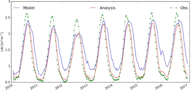
presents a 10-day time series of LAI averaged over the whole domain for the 2010–2016 time period. From Figure2, one can see that the open-loop simulation tends to overestimate the observed LAI in winter periods and that the senescence phase of vegetation is too late over the autumn when compared with the observations. In that respect, the assimilation is efficiently correcting the model; however, analysed LAI does not reach LAI maximal values of the observations. Figure3shows maps of LAI for the model (Figure3a), the observations (Figure3b), and the analysis (Figure3c) averaged over 2010–2016. It is clearly visible that the model overestimates LAI in the eastern part of the domain. Also, some geographical patterns visible in the observations (e.g., the Mississippi area in Figure3b) are not represented in the model (Figure3a). After assimilation, the analysis presents reduced LAI values in the eastern part of the domain and the above-mentioned geographical patterns are visible too (Figure3c). This shows the ability of the assimilation to integrate geographical information into the model. Figure3also presents seasonal scores between the model and the observations and between the analysis and the observations for RMSD and R over the 2010–2016 time period. The analysis leads to a better fit between the model forecasts and the subsequent assimilated observations for both metrics. On average for the whole period, RMSD values drop from 1.10 m2m−2(model vs. observations) to 0.65 m2m−2(analysis vs. observations), while R values increase from 0.69 (model vs. observations) to 0.88 (analysis vs. observations). Figure4presents the same information content for soil moisture. As ESA CCI SSM was rescaled in order to match the first two moments of the modelled SSM cumulative distribution function, the impact is marginal and differences are hardly visible from Figure4a–c. From Figure4d,e, however, one can appreciate the added value of the analysis: RMSD values drop from 0.046 m3m−3(model vs. observations) to 0.044 m3m−3(analysis vs. observations), while R values increase from 0.85 (model vs. observations) to 0.87 (analysis vs. observations). It is worth mentioning that the good level of scores (prior as well as after assimilation) are linked to the rescaling of the ESA CCI SSM data to the model climatology. Finally, Figure5shows maps of analysis increments for 4 (out of 8) control variables averaged over the whole 2010–2016 time period (LAI, second, fourth, and sixth layers of soil from left to right, respectively). It can be noticed that the magnitude of increments is decreasing with depth. It can also be noticed that over almost the whole domain, the analysis tends to add water in the soil near the surface (positive increments), while it dries layers where the roots are mainly located (from layer 4 to 6, negative increments).
Remote Sens.2018,10, 1627 9 of 24
Remote Sens. 2018, 10, x FOR PEER REVIEW 9 of 24
Figure 2. Leaf area index time series from the model (blue line), the observations (green dots and dashed line), and the analysis (red line) averaged over the whole domain from 2010 to 2017.
Figure 3. Top row; leaf area index from (a) the model, (b) the observations, and (c) the analysis averaged over the 2010–2016 time period. Bottom row: seasonal (d) root mean square difference (RMSD) and (e) correlation values between leaf area index (LAI) from the model (in blue), the analysis (in red) and GEOV1 LAI estimates from the Copernicus Global Land Service project from 2010 to 2016.
Figure 2. Leaf area index time series from the model (blue line), the observations (green dots and dashed line), and the analysis (red line) averaged over the whole domain from 2010 to 2017.
Remote Sens. 2018, 10, x FOR PEER REVIEW 9 of 24
Figure 2. Leaf area index time series from the model (blue line), the observations (green dots and dashed line), and the analysis (red line) averaged over the whole domain from 2010 to 2017.
Figure 3. Top row; leaf area index from (a) the model, (b) the observations, and (c) the analysis averaged over the 2010–2016 time period. Bottom row: seasonal (d) root mean square difference (RMSD) and (e) correlation values between leaf area index (LAI) from the model (in blue), the analysis (in red) and GEOV1 LAI estimates from the Copernicus Global Land Service project from 2010 to 2016.
Figure 3.Top row; leaf area index from (a) the model, (b) the observations, and (c) the analysis averaged over the 2010–2016 time period. Bottom row: seasonal (d) root mean square difference (RMSD) and (e) correlation values between leaf area index (LAI) from the model (in blue), the analysis (in red) and GEOV1 LAI estimates from the Copernicus Global Land Service project from 2010 to 2016.
Remote Sens.2018,10, 1627 10 of 24
Remote Sens. 2018, 10, x FOR PEER REVIEW 10 of 24
Figure 4. (a–e) same as Figure 3 for soil moisture.
Figure 5. Analysis increments averaged over the 2010–2016 time period for (a) LAI in m2 m−2, (b)
second, (c) fourth, and (d) sixth layer of soil moisture in m3 m−3. 3.2. Evaluation Using Independent Datasets
3.2.1. Evapotranspiration and GPP
Table 2 presents the statistical scores from the evaluation of both the open-loop and the analysis with respect to evapotranspiration and GPP averaged over 2010–2016, as well as the mean of the evaluation data set over the considered area. On average, R increases from 0.80 to 0.81 when comparing evapotranspiration from the model and from the analysis, respectively, to the independent estimates. Average RMSD decreases from 0.89 kg m−2 d−1 to 0.85 kg m−2 d−1. When
compared with GPP estimates, averaged correlations rise from 0.74 to 0.78 and RMSD drops from 2.20 g(C) m−2 d−1 to 1.91 g(C) m−2 d−1 when considering the model or the analysis, respectively.
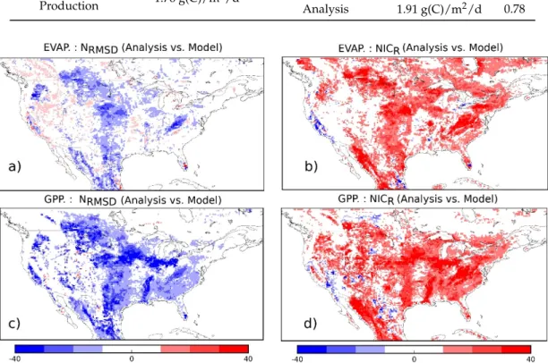
Figure 6 presents spatial maps of NRMSD (Figure 6a,c) and NICR (Figure 6b,d) resulting from the
comparison with evapotranspiration (Figure 6, top row) and GPP (Figure 6, bottom row) of their modelled and analysed equivalent. For NRMSD (Figure 6a,c), blue colours represent an improvement
from the analysis regarding RMSDs (i.e., the latter better represents either evapotranspiration or GPP than the model), while for NICR (Figure 6b,d), red colours depict an improvement from the
analysis. Figure 6 shows that both evapotranspiration and GPP are improved almost everywhere in terms of correlation and RMSD, and that the impact of the assimilation is stronger for GPP than for evapotranspiration. At the seasonal scale (not shown), the assimilation leads to a positive impact all year long in the representation of GPP in terms of both RMSD and R values. Impact from the assimilation on evapotranspiration is smaller (as seen in Table 2), while RMSD values are slightly improved all year long, R values are slightly improved from April to October and slightly degraded from November to March.
Figure 4.(a–e) same as Figure3for soil moisture.
Remote Sens. 2018, 10, x FOR PEER REVIEW 10 of 24
Figure 4. (a–e) same as Figure 3 for soil moisture.
Figure 5. Analysis increments averaged over the 2010–2016 time period for (a) LAI in m2 m−2, (b)
second, (c) fourth, and (d) sixth layer of soil moisture in m3 m−3. 3.2. Evaluation Using Independent Datasets
3.2.1. Evapotranspiration and GPP
Table 2 presents the statistical scores from the evaluation of both the open-loop and the analysis with respect to evapotranspiration and GPP averaged over 2010–2016, as well as the mean of the evaluation data set over the considered area. On average, R increases from 0.80 to 0.81 when comparing evapotranspiration from the model and from the analysis, respectively, to the independent estimates. Average RMSD decreases from 0.89 kg m−2 d−1 to 0.85 kg m−2 d−1. When
compared with GPP estimates, averaged correlations rise from 0.74 to 0.78 and RMSD drops from 2.20 g(C) m−2 d−1 to 1.91 g(C) m−2 d−1 when considering the model or the analysis, respectively.
Figure 6 presents spatial maps of NRMSD (Figure 6a,c) and NICR (Figure 6b,d) resulting from the
comparison with evapotranspiration (Figure 6, top row) and GPP (Figure 6, bottom row) of their modelled and analysed equivalent. For NRMSD (Figure 6a,c), blue colours represent an improvement
from the analysis regarding RMSDs (i.e., the latter better represents either evapotranspiration or GPP than the model), while for NICR (Figure 6b,d), red colours depict an improvement from the
analysis. Figure 6 shows that both evapotranspiration and GPP are improved almost everywhere in terms of correlation and RMSD, and that the impact of the assimilation is stronger for GPP than for evapotranspiration. At the seasonal scale (not shown), the assimilation leads to a positive impact all year long in the representation of GPP in terms of both RMSD and R values. Impact from the assimilation on evapotranspiration is smaller (as seen in Table 2), while RMSD values are slightly improved all year long, R values are slightly improved from April to October and slightly degraded from November to March.
Figure 5. Analysis increments averaged over the 2010–2016 time period for (a) LAI in m2 m−2, (b) second, (c) fourth, and (d) sixth layer of soil moisture in m3m−3.
3.2. Evaluation Using Independent Datasets 3.2.1. Evapotranspiration and GPP
Table2presents the statistical scores from the evaluation of both the open-loop and the analysis with respect to evapotranspiration and GPP averaged over 2010–2016, as well as the mean of the evaluation data set over the considered area. On average, R increases from 0.80 to 0.81 when comparing evapotranspiration from the model and from the analysis, respectively, to the independent estimates. Average RMSD decreases from 0.89 kg m−2 d−1 to 0.85 kg m−2d−1. When compared with GPP estimates, averaged correlations rise from 0.74 to 0.78 and RMSD drops from 2.20 g(C) m−2d−1 to 1.91 g(C) m−2d−1when considering the model or the analysis, respectively. Figure6presents spatial maps of NRMSD (Figure6a,c) and NICR (Figure6b,d) resulting from the comparison with
evapotranspiration (Figure6, top row) and GPP (Figure6, bottom row) of their modelled and analysed equivalent. For NRMSD (Figure 6a,c), blue colours represent an improvement from the analysis
regarding RMSDs (i.e., the latter better represents either evapotranspiration or GPP than the model), while for NICR(Figure6b,d), red colours depict an improvement from the analysis. Figure6shows that
both evapotranspiration and GPP are improved almost everywhere in terms of correlation and RMSD, and that the impact of the assimilation is stronger for GPP than for evapotranspiration. At the seasonal scale (not shown), the assimilation leads to a positive impact all year long in the representation of GPP in terms of both RMSD and R values. Impact from the assimilation on evapotranspiration is smaller (as seen in Table 2), while RMSD values are slightly improved all year long, R values are slightly improved from April to October and slightly degraded from November to March.
Remote Sens.2018,10, 1627 11 of 24
Table 2.Statistical scores from the evaluation of both the open-loop and the analysis with respect to evapotranspiration and gross primary production (GPP) averaged over 2010–2016. RMSD—root mean square difference.
Mean of the
Evaluation Data Set Experiments RMSD R
Evapotranspiration 1.46 kg/m2/d Open-loop 0.87 kg/m 2/d 0.80 Analysis 0.85 kg/m2/d 0.81 Gross Primary Production 1.76 g(C)/m 2/d Open-loop 2.20 g(C)/m 2/d 0.74 Analysis 1.91 g(C)/m2/d 0.78
Remote Sens. 2018, 10, x FOR PEER REVIEW 11 of 24 Table 2. Statistical scores from the evaluation of both the open-loop and the analysis with respect to evapotranspiration and gross primary production (GPP) averaged over 2010–2016. RMSD—root mean square difference.
Mean of the Evaluation Data Set Experiments RMSD R Evapotranspiration 1.46 kg/m2/d Open-loop 0.87 kg/m
2/d 0.80
Analysis 0.85 kg/m2/d 0.81
Gross Primary Production 1.76 g(C)/m2/d Open-loop 2.20 g(C)/m
2/d 0.74
Analysis 1.91 g(C)/m2/d 0.78
Figure 6. Top row: (a) normalized root mean square difference (RMSD) (blue colours indicate an improvement) and (b) normalized information contribution (NIC) applied on correlations values (red colours indicate an improvement) for evapotranspiration from the analysis with respect to the model. Bottom row: same as top row for gross primary production. Units are percentages.
Geographical patterns, as seen on the middle of Figure 6a,c (transition from relative wet to dry areas) areas of the Midwest, are also visible in the soil moisture increments maps of Figure 5b,c, where stronger increments occur. It is difficult to state whether or not those strong corrections reflect atmospheric forcing errors, for example, precipitation, in this area as to date, very few studies have evaluated ERA5 precipitation errors. Ref. [52] have evaluated a large amount of precipitation products, including ERA5, using the high-resolution (4 km) stage-IV gauge-radar precipitation data set as a reference over CONUS using several metrics for 2008–2017. Figure 1d of [52], illustrates the Kling–Gupta efficiency (KGE) scores between ERA5 precipitation and stage-IV reference. If lower values seem to be observed in the above-mentioned transition area, it is not clear enough to incriminate precipitation errors. However, this geographical pattern corresponds to a specific soil moisture regime, the Ustic regime, where moisture is present in the soil, but limited, at times in which conditions are suitable for plant growth (as visible on the following USDA map: https://www.nrcs.usda.gov/Internet/FSE_MEDIA/nrcs142p2_050436.jpg, last access October 2018). This area has specific soil properties including clay, with high swelling potential [53]. Such soil properties are likely to be misrepresented in the model, possibly leading to stronger increments in the analysis.
Figure 6. Top row: (a) normalized root mean square difference (RMSD) (blue colours indicate an improvement) and (b) normalized information contribution (NIC) applied on correlations values (red colours indicate an improvement) for evapotranspiration from the analysis with respect to the model. Bottom row: same as top row for gross primary production. Units are percentages.
Geographical patterns, as seen on the middle of Figure6a,c (transition from relative wet to dry areas) areas of the Midwest, are also visible in the soil moisture increments maps of Figure 5b,c, where stronger increments occur. It is difficult to state whether or not those strong corrections reflect atmospheric forcing errors, for example, precipitation, in this area as to date, very few studies have evaluated ERA5 precipitation errors. Ref. [52] have evaluated a large amount of precipitation products, including ERA5, using the high-resolution (4 km) stage-IV gauge-radar precipitation data set as a reference over CONUS using several metrics for 2008–2017. Figure 1d of [52], illustrates the Kling–Gupta efficiency (KGE) scores between ERA5 precipitation and stage-IV reference. If lower values seem to be observed in the above-mentioned transition area, it is not clear enough to incriminate precipitation errors. However, this geographical pattern corresponds to a specific soil moisture regime, the Ustic regime, where moisture is present in the soil, but limited, at times in which conditions are suitable for plant growth (as visible on the following USDA map:https://www.nrcs.usda.gov/ Internet/FSE_MEDIA/nrcs142p2_050436.jpg, last access October 2018). This area has specific soil properties including clay, with high swelling potential [53]. Such soil properties are likely to be misrepresented in the model, possibly leading to stronger increments in the analysis.
Remote Sens.2018,10, 1627 12 of 24
3.2.2. Soil Moisture
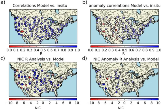
The statistical scores for surface soil moisture from the model and the analysis (third layer of soil between 4 and 10 cm depth) over 2010–2016 when compared with ground measurements from the USCRN network (at 5 cm depth) are presented in Table3. Median R values on volumetric soil moisture time-series (anomaly time series), along with their 95% confidence interval of the median, derived from 10,000-sample bootstrapping are as follows: 0.72±0.02 (0.60±0.02) and 0.74±0.02 (0.60±0.02), while median ubRMSDs are 0.049 ±0.004 and 0.048±0.004 for the model and the analysis, respectively. Figure7a,b illustrate correlation values on volumetric and anomaly time-series between the model and the observations, respectively, for each station. Figure7c,d represent the added value of the analysis expressed through the NIC index (Equation (1)) applied for correlations (NICR)
values on volumetric and anomaly time-series; large blue circles represent a positive impact from the analysis at NICRgreater that +3 (i.e., R values are better when the analysis is used than when
the model is used), large red circles a degradation from the analysis at NICRsmaller than−3, while
diamond symbols represent a rather neutral impact at NICRin between [−3; +3]. While 46% (81%) of
the pool of stations present a rather neutral impact for R values on volumetric (anomaly) time series, stations more impacted by the analysis tend to be positively impacted at 46% (18%), to be compared with 8% (1%) of negative impacts. Although differences between the model run and the analysis are rather small, these results underline the added value of the analysis with respect to the model run.
Remote Sens. 2018, 10, x FOR PEER REVIEW 12 of 24 3.2.2. Soil Moisture
The statistical scores for surface soil moisture from the model and the analysis (third layer of soil between 4 and 10 cm depth) over 2010–2016 when compared with ground measurements from the USCRN network (at 5 cm depth) are presented in Table 3. Median R values on volumetric soil moisture time-series (anomaly time series), along with their 95% confidence interval of the median, derived from 10,000-sample bootstrapping are as follows: 0.72 ± 0.02 (0.60 ± 0.02) and 0.74 ± 0.02 (0.60 ± 0.02), while median ubRMSDs are 0.049 ± 0.004 and 0.048 ± 0.004 for the model and the analysis, respectively. Figure 7a,b illustrate correlation values on volumetric and anomaly time-series between the model and the observations, respectively, for each station. Figure 7c,d represent the added value of the analysis expressed through the NIC index (Equation (1)) applied for correlations (NICR) values on volumetric and anomaly time-series; large blue circles represent a
positive impact from the analysis at NICR greater that +3 (i.e., R values are better when the analysis
is used than when the model is used), large red circles a degradation from the analysis at NICR
smaller than −3, while diamond symbols represent a rather neutral impact at NICR in between [−3;
+3]. While 46% (81%) of the pool of stations present a rather neutral impact for R values on volumetric (anomaly) time series, stations more impacted by the analysis tend to be positively impacted at 46% (18%), to be compared with 8% (1%) of negative impacts. Although differences between the model run and the analysis are rather small, these results underline the added value of the analysis with respect to the model run.
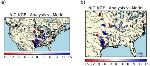
Figure 7. Maps of correlation (R) on volumetric time-series (a) and anomaly time-series (b) between in situ measurements at 5 cm depth from the US Climate Reference Network (USCRN) network and soil moisture from the model (third layer of soil between 4 cm and 10 cm) from 2010 to 2016. NIC applied on R (anomaly R) values (c,d); analysis with respect to the model. NIC scores are classified according to three categories: (i) negative impact from the analysis with respect to the model with values smaller than −3% (red circles), (ii) positive impact from the analysis with respect to the model with values greater than +3% (blue circles), and (iii) neutral impact from the analysis with respect to the model with values between −3% and 3% (diamonds).
Figure 7.Maps of correlation (R) on volumetric time-series (a) and anomaly time-series (b) between in situ measurements at 5 cm depth from the US Climate Reference Network (USCRN) network and soil moisture from the model (third layer of soil between 4 cm and 10 cm) from 2010 to 2016. NIC applied on R (anomaly R) values (c,d); analysis with respect to the model. NIC scores are classified according to three categories: (i) negative impact from the analysis with respect to the model with values smaller than−3% (red circles), (ii) positive impact from the analysis with respect to the model with values greater than +3% (blue circles), and (iii) neutral impact from the analysis with respect to the model with values between−3% and 3% (diamonds).
Remote Sens.2018,10, 1627 13 of 24
Table 3.Analysis impact evaluation against in situ measurements of soil moisture from the US Climate Reference Network (USCRN) network. In situ measurements at a depth of 5 cm are used to evaluate soil moisture from the third layer of soil (4–10 cm) from either the model or analysis experiment over 2010–2016. The normalized information contribution (NIC) is applied to the correlation (anomaly correlations) values. NIC scores are classified according to three categories: (i) negative impact from the analysis with respect to the model with values smaller than−3%, (ii) positive impact from the analysis with respect to the model with values greater than +3%, and (iii) neutral impact from the analysis with respect to the model with values between−3% and 3%.
110 (110) Stations with Significant R (Anomaly R) Median R (Anomaly R) Median ubRMSD Positive Impact: >+3 ←3 Negative Impact: <−3 Neutral Impact [−3; +3] Model 0.72±0.02 * (0.60±0.02 *) 0.049±0.004
* N/A N/A N/A
Analysis 0.74±0.02 * (0.60±0.02 *)
0.048±0.004
* 46% (18%) 8% (1%) 46% (81%)
* 95% confidence interval of the median derived from a 10,000 samples bootstrapping.
3.2.3. Streamflow
A subset of 258 out of 531 gauging stations was selected for the evaluation according to the criteria described in the methodology section, with KGE scores within the [0, 1] interval. Figure8presents the performance of analysed streamflow with respect to the one from the model run for this pool of stations, with a focus on the eastern part of the domain. NICKGEvalues are presented following
the same classification as NICRapplied to soil moisture. Scores are presented in Table4. Looking at
NICKGE, 62% of the pool of stations (258 stations) present a rather neutral impact (at NICKGEbetween
[−3; 3]) and 26% of the stations present a positive impact (at NICKGE> +3), while only 12% of stations
have a negative impact (at NICKGE<−3). NICR, NREσ, and NREµfollow the same classification (with even a smaller percentage of stations being negatively affected by the analysis; 1%); when the analysis is impacting streamflow representation, it tends to be a positive impact.
Remote Sens. 2018, 10, x FOR PEER REVIEW 13 of 24 Table 3. Analysis impact evaluation against in situ measurements of soil moisture from the US Climate Reference Network (USCRN) network. In situ measurements at a depth of 5 cm are used to evaluate soil moisture from the third layer of soil (4–10 cm) from either the model or analysis experiment over 2010–2016. The normalized information contribution (NIC) is applied to the correlation (anomaly correlations) values. NIC scores are classified according to three categories: (i) negative impact from the analysis with respect to the model with values smaller than −3%, (ii) positive impact from the analysis with respect to the model with values greater than +3%, and (iii) neutral impact from the analysis with respect to the model with values between −3% and 3%.
110 (110) Stations with Significant R (Anomaly R) Median R (Anomaly R) Median ubRMSD Positive Impact: >+3 ←3 Negative Impact: <−3 Neutral Impact [−3; +3] Model 0.72 ± 0.02 *
(0.60 ± 0.02 *) 0.049 ± 0.004 * N/A N/A N/A
Analysis 0.74 ± 0.02 *
(0.60 ± 0.02 *) 0.048 ± 0.004 * 46% (18%) 8% (1%) 46% (81%) * 95% confidence interval of the median derived from a 10,000 samples bootstrapping.
3.2.3. Streamflow
A subset of 258 out of 531 gauging stations was selected for the evaluation according to the criteria described in the methodology section, with KGE scores within the [0, 1] interval. Figure 8 presents the performance of analysed streamflow with respect to the one from the model run for this pool of stations, with a focus on the eastern part of the domain. NICKGE values are presented
following the same classification as NICR applied to soil moisture. Scores are presented in Table 4.
Looking at NICKGE, 62% of the pool of stations (258 stations) present a rather neutral impact (at
NICKGE between [−3; 3]) and 26% of the stations present a positive impact (at NICKGE > +3), while
only 12% of stations have a negative impact (at NICKGE < −3). NICR, NREσ, and NREμ follow the same
classification (with even a smaller percentage of stations being negatively affected by the analysis; 1%); when the analysis is impacting streamflow representation, it tends to be a positive impact.
Figure 8. Normalized information contribution scores based on Kling–Gupta efficiency (KGE) scores (NICKGE) (a) analysis with respect to the model, (b) zoom over the eastern part of the domain. Small
diamonds represent stations for which NICKGE are between [−3; +3]. NICKGE greater than 3 (blue
large circles) suggest an improvement from the analysis over the model, values smaller than −3 (red large circles) suggest a degradation. For sake of clarity, a factor of 100 has been applied to NIC.
Figure 8.Normalized information contribution scores based on Kling–Gupta efficiency (KGE) scores (NICKGE) (a) analysis with respect to the model, (b) zoom over the eastern part of the domain. Small diamonds represent stations for which NICKGEare between [−3; +3]. NICKGEgreater than 3 (blue large circles) suggest an improvement from the analysis over the model, values smaller than−3 (red large circles) suggest a degradation. For sake of clarity, a factor of 100 has been applied to NIC.
Remote Sens.2018,10, 1627 14 of 24
Table 4. Analysis impact evaluation against daily streamflow over 2010–2016. The impact from the analysis with respect to the model is assessed through the normalized information contribution (NIC) applied to the Kling–Gupta efficiency (KGE) score, as well as using normalized relative error of simulated or analysed mean (REµ) and standard deviation (REσ). Scores are classified according to three categories: (i) negative impact from the analysis with respect to the model with values smaller than−3, (ii) positive impact from the analysis with respect to the model with values greater than +3, and (iii) neutral impact from the analysis with respect to the model with values between−3 and 3. 258 out of 531 Stations
with KGE Greater than 0 Positive Impact: >+3 Negative Impact: <−3 Neutral Impact [−3; +3]
NICKGE 26% 12% 62%
NREσ 22% 1% 77%
NREµ 34% 1% 65%
4. Potential Applications, Discussions, and Perspectives
4.1. Could LDAS-Monde be Used to Monitor Agricultural Droughts?
The previous section has highlighted the LDAS-Monde ability to enhance the monitoring accuracy for land surface variables. It should then be possible to use it to better represent extreme events like agricultural droughts. Figure9represents monthly LAI anomalies averaged over the U.S. corn belt (simplified as a box from 110◦W to 70◦W and 30◦N to 50◦N) with respect to 2010–2016 means from the model, the analysis, and the observations. As shown by Figure9, for the second part of the year 2012, LAI observations exhibit a strong negative anomaly at this domain scale. While it is also visible in the model, the latter clearly overestimates the intensity of the observed anomaly. The analysed LAI anomaly is closer to the observed one than the model. This extreme drought event is known as the August 2012 U.S. corn belt drought. The U.S. Department of Agriculture (USDA,www.nass.usda.gov, last access June 2018) estimated that corn yield (per acre of planted crop) was 26% below the expectation that they had at the beginning of the 2012 growing season. The 2012 corn yield deficit and the implied climatic impact was classified as a ‘historic event’ [54]. As visible on Figure9, spring 2012 presents a positive anomaly for vegetation. Ref. [55] defined spring 2012 as the earliest false spring in the North American record (i.e., a period of weather in late winter or early spring allowing vegetation to be prematurely brought out of dormancy). This false spring has contributed to an earlier dry out of the soil. Figure10presents maps of the LAI anomaly for this specific month for the model, observations, and analysis from left to right, respectively. Compared with the observations (Figure10b), the area affected by the anomaly in the model (Figure10a) is too large and too intense, while the analysis (Figure10c) better matches the observed pattern in both space and intensity. This impact is valid when compared with most of the severe droughts events that occurred over CONUS (data from the National Oceanic and Atmospheric Administration (NOAA) state of the climate website, last access April 2018
https://www.ncdc.noaa.gov/sotc/drought/201803, not shown). Hence, LDAS-Monde provides a better tool than the model alone to monitor extreme events like agricultural droughts.
Remote Sens. 2018, 10, x FOR PEER REVIEW 14 of 24 Table 4. Analysis impact evaluation against daily streamflow over 2010–2016. The impact from the analysis with respect to the model is assessed through the normalized information contribution (NIC) applied to the Kling–Gupta efficiency (KGE) score, as well as using normalized relative error of simulated or analysed mean (REμ) and standard deviation (REσ). Scores are classified according to
three categories: (i) negative impact from the analysis with respect to the model with values smaller than −3, (ii) positive impact from the analysis with respect to the model with values greater than +3, and (iii) neutral impact from the analysis with respect to the model with values between −3 and 3.
258 out of 531 Stations with KGE Greater than 0
Positive Impact: >+3 Negative Impact: <−3 Neutral Impact [−3; +3] NICKGE 26% 12% 62% NREσ 22% 1% 77% NREμ 34% 1% 65%
4. Potential Applications, Discussions, and Perspectives 4.1. Could LDAS-Monde be Used to Monitor Agricultural Droughts?
The previous section has highlighted the LDAS-Monde ability to enhance the monitoring accuracy for land surface variables. It should then be possible to use it to better represent extreme events like agricultural droughts. Figure 9 represents monthly LAI anomalies averaged over the U.S. corn belt (simplified as a box from 110°W to 70°W and 30°N to 50°N) with respect to 2010–2016 means from the model, the analysis, and the observations. As shown by Figure 9, for the second part of the year 2012, LAI observations exhibit a strong negative anomaly at this domain scale. While it is also visible in the model, the latter clearly overestimates the intensity of the observed anomaly. The analysed LAI anomaly is closer to the observed one than the model. This extreme drought event is known as the August 2012 U.S. corn belt drought. The U.S. Department of Agriculture (USDA, www.nass.usda.gov, last access June 2018) estimated that corn yield (per acre of planted crop) was 26% below the expectation that they had at the beginning of the 2012 growing season. The 2012 corn yield deficit and the implied climatic impact was classified as a ‘historic event’ [54]. As visible on Figure 9, spring 2012 presents a positive anomaly for vegetation. Ref. [55] defined spring 2012 as the earliest false spring in the North American record (i.e., a period of weather in late winter or early spring allowing vegetation to be prematurely brought out of dormancy). This false spring has contributed to an earlier dry out of the soil. Figure 10 presents maps of the LAI anomaly for this specific month for the model, observations, and analysis from left to right, respectively. Compared with the observations (Figure 10b), the area affected by the anomaly in the model (Figure 10a) is too large and too intense, while the analysis (Figure 10c) better matches the observed pattern in both space and intensity. This impact is valid when compared with most of the severe droughts events that occurred over CONUS (data from the National Oceanic and Atmospheric Administration (NOAA) state of the climate website, last access April 2018 https://www.ncdc.noaa.gov/sotc/drought/201803, not shown). Hence, LDAS-Monde provides a better tool than the model alone to monitor extreme events like agricultural droughts.
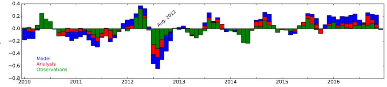
Figure 9. Leaf area index (LAI) monthly anomalies over the 2010–2016 time period for the model (blue bars), the analysis (red bars), and the CGLS GEOV1 observations (in green) over the corn belt drought defined as a box from 110°W to 70°W and 30°N to 50°N.
Figure 9.Leaf area index (LAI) monthly anomalies over the 2010–2016 time period for the model (blue bars), the analysis (red bars), and the CGLS GEOV1 observations (in green) over the corn belt drought defined as a box from 110◦W to 70◦W and 30◦N to 50◦N.
Remote Sens.2018,10, 1627 15 of 24
Remote Sens. 2018, 10, x FOR PEER REVIEW 15 of 24
Figure 10. (a) Monthly anomaly of leaf area index for August 2012 with respect to the 2010–2016 period, (b) same as (a) for observed leaf area index, and (c) same as (a) for analysed leaf area index.
It is also worth mentioning that if LDAS-Monde brings a clear improvement in the representation of LAI, reducing the overestimation duration as well as the minimal values, as its model counterpart, it fails capturing the observed LAI peak intensity. Ref. [13] has evaluated the model sensitivity of the observation for Europe over 2000–2012 reflected in the SEKF Jacobians. The Jacobians depend on the model physics and their examination provides useful insight that explains the data assimilation system performances [21,56]. Ref. [13] suggests a seasonal dependency of the model sensitivity to the observed LAI. High sensitivity is found in autumn. Smaller model sensitivity at the time of the year where the peak LAI occurs (late spring) prevails the analysis to match the observations correctly.
As highlighted by [57], who have evaluated the capacity of several LSMs (including ISBA) to accurately simulate observed energy and water fluxes during droughts, there is a need to re-examine existing model components in LSMs to improve simulations of soil hydrological processes and water–plant interactions. It appears from Figure 2 that although the analysis is able to correct the overestimated LAI values in winter, the minimum LAI thresholds used in ISBA has to be revisited. Recently, the satellite derived LAI data have been disaggregated following a Kalman filtering technique developed by [58]. This enables the LAI signal for each vegetation type to be separated within the pixel, which provides a dynamic vegetation-dependent estimate of the assimilated LAI within the pixel [59]. This new dataset will make it possible to modify the minimum LAI thresholds accordingly.
4.2. Could LDAS-Monde Provide Accurate Initial Conditions for Vegetation Forecasts?
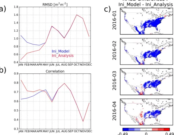
In the context of NWP, assimilation of satellite observations in atmospheric models has the capacity to mitigate model deficiencies, leading to better estimates of system states. This has been the main driver of the improvement of both weather forecast skill and lead time [60]. Data assimilation is able to produce similar benefits for LSVs forecasting. Seeking to foster a link with applications, LDAS-Monde could not only be used to monitor the LSVs, but could also be integrated into a forecasting system (at different time scales) assuming that it can provide better initial conditions than a model run and that its impact lasts in time. Many applications could benefit from a better representation of the LSVs, from NWP [61], to early warning systems of, for example, agricultural drought and yield forecasts. As a first step towards such early warning systems, Figure 11 shows a comparison between LAI from the two last simulations presented in Table 1: Ini_Model and Ini_Analysis. Figure 11a,b shows monthly RMSD (R) values for the year 2016 for LAI. A strong impact is visible not only from the beginning of the two simulations, but also a few months later (up to April). The four maps of Figure 11c show RMSD differences between Ini_analysis and Ini_model from January to April. All maps are dominated by negative values (in blue), suggesting that Ini_analysis presents a better match with the observed LAI and that analysis effects last in time. Southeastern part of the domain is mainly affected, these areas are dominated by broadleaves forest as well as C3 crops. Large differences between the model and the analysis during winter time (as shown on Figure 2) suggest that the minimum LAI threshold used in the model for these vegetation types has to be revisited. Such results are strongly linked to the time of the year when the
Figure 10.(a) Monthly anomaly of leaf area index for August 2012 with respect to the 2010–2016 period, (b) same as (a) for observed leaf area index, and (c) same as (a) for analysed leaf area index.
It is also worth mentioning that if LDAS-Monde brings a clear improvement in the representation of LAI, reducing the overestimation duration as well as the minimal values, as its model counterpart, it fails capturing the observed LAI peak intensity. Ref. [13] has evaluated the model sensitivity of the observation for Europe over 2000–2012 reflected in the SEKF Jacobians. The Jacobians depend on the model physics and their examination provides useful insight that explains the data assimilation system performances [21,56]. Ref. [13] suggests a seasonal dependency of the model sensitivity to the observed LAI. High sensitivity is found in autumn. Smaller model sensitivity at the time of the year where the peak LAI occurs (late spring) prevails the analysis to match the observations correctly.
As highlighted by [57], who have evaluated the capacity of several LSMs (including ISBA) to accurately simulate observed energy and water fluxes during droughts, there is a need to re-examine existing model components in LSMs to improve simulations of soil hydrological processes and water–plant interactions. It appears from Figure2that although the analysis is able to correct the overestimated LAI values in winter, the minimum LAI thresholds used in ISBA has to be revisited. Recently, the satellite derived LAI data have been disaggregated following a Kalman filtering technique developed by [58]. This enables the LAI signal for each vegetation type to be separated within the pixel, which provides a dynamic vegetation-dependent estimate of the assimilated LAI within the pixel [59]. This new dataset will make it possible to modify the minimum LAI thresholds accordingly. 4.2. Could LDAS-Monde Provide Accurate Initial Conditions for Vegetation Forecasts?
In the context of NWP, assimilation of satellite observations in atmospheric models has the capacity to mitigate model deficiencies, leading to better estimates of system states. This has been the main driver of the improvement of both weather forecast skill and lead time [60]. Data assimilation is able to produce similar benefits for LSVs forecasting. Seeking to foster a link with applications, LDAS-Monde could not only be used to monitor the LSVs, but could also be integrated into a forecasting system (at different time scales) assuming that it can provide better initial conditions than a model run and that its impact lasts in time. Many applications could benefit from a better representation of the LSVs, from NWP [61], to early warning systems of, for example, agricultural drought and yield forecasts. As a first step towards such early warning systems, Figure11shows a comparison between LAI from the two last simulations presented in Table1: Ini_Model and Ini_Analysis. Figure11a,b shows monthly RMSD (R) values for the year 2016 for LAI. A strong impact is visible not only from the beginning of the two simulations, but also a few months later (up to April). The four maps of Figure11c show RMSD differences between Ini_analysis and Ini_model from January to April. All maps are dominated by negative values (in blue), suggesting that Ini_analysis presents a better match with the observed LAI and that analysis effects last in time. Southeastern part of the domain is mainly affected, these areas are dominated by broadleaves forest as well as C3 crops. Large differences between the model and the analysis during winter time (as shown on Figure2) suggest that the minimum LAI threshold used in the model for these vegetation types has to be revisited. Such results are strongly linked to the time of the year when the simulation is initialised by the analysis, that is, the greater the prior