Forecasting indoor temperatures during heatwaves using time series models

(1)

Contents lists available atScienceDirect

Building and Environment

journal homepage:www.elsevier.com/locate/buildenv

Forecasting indoor temperatures during heatwaves using time series models

Matej Gustin

a,b,∗

, Robert S. McLeod

a,b

, Kevin J. Lomas

a,b

a_{School of Architecture, Building and Civil Engineering, Loughborough University, LE11 3TU, UK}

b_{London-Loughborough (LoLo) EPSRC Centre for Doctoral Training in Energy Demand, Loughborough University, LE11 3TU, UK}

A R T I C L E I N F O Keywords:

Time series forecasting Machine learning Black-box model ARX model ARMAX model Overheating A B S T R A C T

Early prediction of impending high temperatures in buildings could play a vital role in reducing heat-related morbidity and mortality. A recursive, AutoRegressive time series model using eXogenous inputs (ARX) and a rolling forecasting origin has been developed to provide reliable short-term forecasts of the internal tempera-tures in dwellings during hot summer conditions, especially heatwaves. The model was tested using monitored data from three case study dwellings recorded during the 2015 heatwave. The predictor variables were selected by minimising the Akaike Information Criterion (AIC), in order to automatically identify a near-optimal model. The model proved capable of performing multi-step-ahead predictions during extreme heat events with an ac-ceptable accuracy for periods up to 72 h, with hourly results achieving a Mean Absolute Error (MAE) below 0.7 °C for every forecast. Comparison betweenARXand AutoRegressive Moving Average models with eXogenous inputs (ARMAX) models showed that theARXmodels provided consistently more reliable multi-step-ahead predictions. Prediction intervals, at the 95% probability level, were adopted to deﬁne a credible interval for the forecast temperatures at diﬀerent prediction horizons. The results point to the potential for using time series forecasting as part of an overheating early-warning system in buildings housing vulnerable occupants or con-tents.

1. Introduction

1.1. Background

Overheating in homes and residential care facilities is increasingly acknowledged as a serious problem for developers, property owners/ managers, landlords, tenants, health care providers and policy makers [1–3]. Climate change projections indicate that the majority of the world's most populated regions will experience more frequent and more intense heat wave periods over the coming decades [4,5]. Warmer than average summers coupled with an increased frequency of extreme heat wave events [6] pose obvious risk factors in relation to overheating in the built environment.

By 2040 average summertime temperatures in the UK are expected to reﬂect those experienced during the heatwave of 2003 [7,8]; an event which caused over 2000 heat-related deaths in the UK and more than 30,000 across Europe [9]. Those most aﬀected by excess heat are the elderly (over the age of 60 years), who are at an increased risk of heat-related illness [10] with those over the age of 65 years having a higher risk of heat-related mortality [11]. Because of the rising average life expectancy in the UK and other developed nations [12], premature mortality rates are an-ticipated to increase when similar events occur in the future.

It is well established that in a temperate climate high ambient temperatures are associated with an increased mortality rate [15,16]. In response to growing concerns regarding global warming and the pre-dicted increase in the frequency of extreme heat-related events, heat plans have been created in a number of countries worldwide in order to establish a collaboration between meteorological services, civil pro-tection and public health authorities to inform and protect residents from the impending health risks of hot weather [11]. Such plans are known as Heat-Health Warning Systems (HHWSs) and are activated when the weather is forecasted to exceed certain thresholds that might lead to adverse health effects. HHWSs are intended to make emergency responses more efficient and better coordinated in order to reduce heat-related morbidity and mortality [12]. It is well known that people in developed countries tend to spend most of their time indoors [13], and it has been established that even healthy people situated indoors are at a significantly higher risk of experiencing adverse conditions of extreme heat than the same healthy individuals would be if they were located outdoors [14]. Since HHWSs are based solely on the outdoor weather conditions and because these warnings are triggered on a regional or national level, it is impossible to accurately identify which dwellings or people are actually at risk.

Excess heat-related deaths can largely be attributed to respiratory

https://doi.org/10.1016/j.buildenv.2018.07.045

Received 17 April 2018; Received in revised form 23 July 2018; Accepted 25 July 2018

∗_{Corresponding author. School of Architecture, Building and Civil Engineering, Loughborough University, LE11 3TU, UK.} E-mail address:[email protected](M. Gustin).

Available online 27 July 2018

(2)

diseases and cardiovascular causes, including: strokes, coronary heart diseases and congestive heart failures [13,14]. However, a study by Rooney et al. [15] observed that mortality during heatwaves occurring late in the summer is lower than at the beginning of the summer; a

finding which suggests that seasonal acclimatisation processes may increase resilience to heat stress. People living in different regions, ci-ties, urban and rural areas are accustomed to different temperatures and respond to heat differently [16]. Coupled with the fact that indoor thermal conditions do not depend solely on the external weather con-ditions, but also on the building characteristics and occupant beha-viour, it is clear that associating heat-related risks exclusively with external temperature thresholds at a regional or national level is in-adequate and that the development of local, dwelling-based thresholds, should be a priority [17].

Despite strong epidemiological correlations between elevated ex-ternal temperatures and increased risks of heat-related morbidity and mortality [18], relatively little is known about the health impacts in residential buildings, and this has been identified as an area requiring further research [19]. Since the overheating criteria currently used in the built environment are based on thermal comfort and not health, the definition and incorporation of heat-safety metrics are required to as-sess heat stress in dwellings [19]. The positive correlation between core body temperatures and indoor temperatures [20], points to the poten-tial of developing indoor health indices based directly on indoor tem-peratures. With the development of dwelling-based indoor thresholds that would associate heat-related risks directly to the indoor environ-mental conditions, predictive models could play an important role as part of a real-time warning device that would allow the timely detection of critical indoor thresholds. Knowing when such thresholds were likely to be breached in specific spaces would allow carers or facility man-agers to warn occupants when health-endangering environmental conditions are expected to occur. If widely deployed, such a system could help to avoid or reduce heat-related morbidity and mortality occurring during hot weather conditions and in the case of dwellings with vulnerable occupants, such a system could trigger the prompt dispatch of the emergency services.

Recent studies related to overheating in dwellings can be broadly divided into three categories:firstly, studies that have involved mea-suring internal air temperatures (and other physical variables) in order to identify and quantify the risk of overheating [21–24]; secondly, those that involved either quasi-steady state or dynamic thermal simulation modelling to assess the current and future risk of overheating [23,25–28]; and lastly, studies that have used empirical data to con-struct forecasting models for the prediction of the indoor thermal conditions [29–33]. The availability of observed data from large mon-itoring studies [21–23,28,34] provides the potential to develop em-pirical models which make predictions based on the data alone (i.e. machine learning). Machine learning models (which lack explicit phy-sical parameterisation) are often referred to as black-box models or more generally as statistical models [35,36]. Such models have the potential to be used in forecasting the short-term future internal tem-peratures in buildings based solely on the external climate data and previously recorded internal temperatures. As such, black-box models are computationally and resource efficient and do not require any physical information describing the room or building fabric. If proven reliable, such models could be usefully deployed to protect building occupants from the impending risks of overheating in a specific space. Provision of tailored information to occupants (or their carers) and/or facilities managers advising on the level of preventative action needed to mitigate the risks is then possible.

1.2. Modelling methods

Diﬀerent types of black-box models can be adopted for the

prediction of internal air temperatures, with the most common being Time Series and Artificial Neural Network (ANN) models [37]. Whereas simpler time series forecasting models are based on linear methods, ANN allows more complex non-linear relationships between the re-sponse variable and its predictors [38]. Nevertheless,ANNmodels are harder to train, require large amounts of learning data and are limited by their lack of interpretability [36]. In addition, ANN models are known to give different results after repeated trials on the same data [30]. For these reasons, linear time series models offer several ad-vantages over their non-linearANNcounterparts: namely that they are simpler to deploy, and the same data and inputs will always produce the same model parameterisation [30].

Ashtiani et al. [32] observed that their time series regression model was not able to forecast accurately during a heatwave event, with the best model achieving anRMSEof 2.10 °C, which points to the difficulty of developing a reliable forecasting model that is able to generalise with acceptable accuracy during such extreme events. Time series fore-casting models such as AutoRegressive models with eXogenous inputs (ARX) and AutoRegressive Moving Average models with eXogenous inputs (ARMAX) have been shown to provide reasonably accurate short-term forecasts (2–3 h) of internal temperatures in office buildings when using high-resolution data (i.e. 5–15 min sampling); such models have achieved a Root Mean Square Error (RMSE) of 0.33 °C for 3-h forecasts using ARX models [33] and a Mean Absolute Error (MAE) of 0.11–0.19 °C for a 2-h forecasts usingARMAXmodels [30]. However, in these studies [30,33], forecasts were made for relatively mild summer days without sudden temperature spikes, and with peak indoor tem-peratures of approximately 24 °C [30] to 26°C [33]. Although the forecasting accuracy of the models developed in the studies was good [30,33], they have been primarily developed to improve HVAC system control in air-conditioned offices and schools where there is detailed information available regarding their operation. As such their use cannot be directly transposed to free-running dwellings where HVAC systems are not generally used or to dwellings where space conditioning is used but operation schedules are far more unpredictable than in

of-ﬁces. Moreover, the use of sub-hourly data which HVAC system control development is predicated upon assumes that there is widespread availability of such high-resolution data and weather forecasts. In rea-lity, if the models were to be integrated as a part of an indoor heat warning device, and deployed on a large scale, using forecasted weather data from national meteorological services, such as the UK Met Oﬃce, weather forecasts are not available at a sub-hourly resolution. Consequently, there is a lack of literature in relation to the development and prototyping of predictive models in relation to forecasting indoor temperatures over extended forecasting horizons that are able to op-erate at an hourly data resolution in free-running dwellings and with acceptable forecasting accuracy during extreme hot spells.

It is well known in forecasting that predictions are diﬃcult to per-form where the values of future predictors fall outside the range of the past (training) values [38]. Hence, if models are not validated over a suitably hot spell it is uncertain whether they would be able to forecast accurately during a heatwave.

In a study by Ríos-Moreno et al. [29], it was found that for pre-dictions of the internal temperature,ARXmodels generally performed more accurately than ARMAX models. Nonetheless, only one-step-ahead forecasts were performed in this study. On the other hand, Mustafaraj et al. [31] found thatARXandARMAXmodels produced similar results, with ARMAXmodels being preferable for multi-step-ahead forecasts. Hence it is unclear from the literature which type of model is capable of providing the most accurate and consistent pre-dictions of internal temperatures during heat waves, especially during extended forecasting horizons.

When longer forecasting horizons (h) are desired, multi-step-ahead forecasts (i.e. advanced predictions of multiple time steps) are required.

(3)

For this purpose, either recursive or direct strategies can be adopted [39]. In a direct strategy, a separate model is trained and adopted for each forecasting horizon [40], using similar methods to those used for one-step-ahead predictions, but with a longer prediction step [41]. In a recursive strategy, the prediction from a one-step-ahead model is used as an input for future prediction horizons [39] and subsequent pre-dictions are performed by simply reiterating short-term predictors [41]. Whereas direct strategies might be superior for mis-specified models (i.e. when the considered class of models is sub-optimal and fails to account for the relationship between the explanatory and response variables1), a recursive strategy may be better suited for well-specified models [40] and for long-range forecasting [42]. In addition, a huge advantage of the recursive strategy is that only one model is required, which considerably reduces the computational time, especially when many inputs are adopted and continuous long-range forecasting outputs are required [40]. Conversely, recursive forecasting is known to pro-duce biased predictions when the underlying model is non-linear, particularly at longer horizons [40]. This is because any uncertainty or error generated in the one-step-ahead prediction accumulates with each subsequent multi-step-ahead prediction, making accurate predictions at longer forecasting horizons more difficult [39]. It is extremely im-portant for this reason, that the base model is properly identified by selecting a near-optimal model that correctly explains the relationship between the explanatory and response variables.

Trial and error identification procedures have been previously adopted for model selection [29,31]. Approaches involving selecting all (or significant numbers) of the potential predictors are unlikely to re-present the best model because of the potential to include non-sig-nificant predictors; conversely, an insufficient number of model pre-dictors might lead to poor performance in multi-step-ahead forecasts. Identifying a near-optimal model manually is therefore a difficult and time-consuming (and potentially impossible) task; and consequently, it is preferable to adopt an automated parameter selection processes.

In the present work, the use of a simple automated model selection procedure designed for the calibration ofARXmodels is demonstrated to provide accurate one-step-ahead, i.e. hourly (1 h), predictions of the internal temperature evolution during a heatwave. A recursive strategy using sliding training and validation windows is adopted to provide hourly multi-step-ahead predictions for different forecasting horizons at: 3 h, 6 h, 12 h, 24 h, 48 h and 72 h periods. The forecasting accuracy and the 95% prediction intervals for the different forecasting horizons are evaluated using data from three different dwellings. The predictions across the various forecasting horizons were then repeated using ARMAX models in order to compare the forecasting accuracy and consistency of the results. The primary aim of this study is to assess the relative ability ofARXandARMAXmodels to generate reliable multi-step-ahead temperature predictions.

2. Data selection

To stress test the predictive capabilities of a model in the context of ‘real-world’overheating predictions, it is important that the model is tested and validated during a hot period in which external temperatures exceed those experienced during the previous (model training) period. According to the UK Met Office, based on the World Meteorological Organization definition, a heatwave is defined as a period of,“marked unusual hot weather (Max, Min and daily average) over a region per-sisting at least two consecutive days during the hot period of the year based on local climatological conditions, with thermal conditions re-corded above given thresholds” [43,44]. For this purpose, three dwellings from the REFIT Smart Home dataset [34] were selected. The houses, all located in close proximity to the town of Loughborough in

the English Midlands, experienced high temperatures but with mark-edly diﬀerent temperature proﬁles, during the two-day heatwave of 30th _{June and 1}st_{July 2015. During this short-duration extreme hot} spell, the external air temperatures exceeded 30 °C in most regions of the UK [45]. The maximum external dry-bulb temperatures during that period set a new July record, with the highest temperature of 36.7 °C being observed at the Heathrow weather station [45]. On the hottest day: dwelling A (REFIT dwelling No. 12) exhibited a sudden indoor temperature spike exceeding 30 °C; dwelling B (REFIT dwelling No. 20) displayed a gradual increase in the internal temperatures with a lower peak of 27.6 °C, but with prolonged retention of elevated temperatures above 26 °C during the following night; and dwelling C (REFIT dwelling No. 7) displayed a sharp rise in temperature during the day but with a sudden drop in temperature overnight (Fig. 1).

The internal temperatures were logged at 30-min intervals in the upstairs bedrooms, to capture the most pronounced overheating. The weather data was recorded at the nearby Loughborough University weather station at 15-min intervals. As weather data and forecasts are not usually available in a sub-hourly resolution, and because hourly temperature data is more widely available, as a starting point for this work it was decided to down-sample the data by averaging the sub-hourly values to sub-hourly mean values (centred on each hour). This re-duces the number of time steps required to reach an extended fore-casting horizon, and hence decreases the accumulation of errors due to the adopted recursive strategy in multi-step-ahead forecasts. However, it retains the ability to deﬁne the peak temperature reasonably accu-rately. Since the use of non-scaled data (i.e. non-normalised data) al-lowed more accurate predictions, the input data did not require trans-formation.

The data selected for the training and forecasting undertaken in this study extends across aﬁve-week period from the 1stJune 2015 to the 5th_{July 2015. During the}_ﬁ_{rst half of June, the external air} tempera-tures (Text) were considerably lower (ranging between 4 °C and 24 °C) than later in the month (Fig. 1). In the second half of June the external air temperatures showed a small increase in the daily mean, but with hourly peaks that did not exceed 24 °C until the 30th_{of June, when the} external temperature suddenly increased to 31 °C. During the second day of the heatwave (1st_{July), the temperature rose even further and} reached a peak of almost 36 °C. On the days following the short hot spell, the external daily temperature variations were very similar to those observed before the heatwave. The Global Horizontal Irradiance (GHI) showed similar daily variations before, during and after the heatwave (Fig. 1). Whereas the highest hourlyGHIwas recorded on the 7thJune, when it peaked at almost 900 W/m2, the peak on the 1stJuly was 750 W/m2_{. Therefore, the higher external temperatures during the} hot spell cannot be attributed to an increase in the solar irradiance.

For the whole of June, the internal temperatures (Tint) in the bed-room of dwelling B are consistently (1–3 °C) warmer than in the bed-room in dwelling A, which is 1–3 °C warmer than the bedroom of dwelling C (Fig. 1). The internal temperatures remain below 25 °C, and so would not be considered uncomfortable, until the 30th_{June when all} the rooms reach approximately 26 °C. On the hottest day, 1st _July, dwellings A and C heat up more noticeably than dwelling B, reaching maximal temperatures of 27.6 °C in dwelling B, 28.0 °C in dwelling C and 30.2 °C in dwelling A (Fig. 1).

3. Methods

3.1. Structure of the models

AutoRegressive models require that the input data used for the de-velopment of the model is stationary in order that the distribution of the observed and forecasted values is independent of time [38]. Hence, a time series can be considered stationary if the mean and variance of the data are constant [46] and if there are no signiﬁcant trends and sea-sonal variations in the data [38]. To objectively determine if the data is 1_{These are typically regression models which may omit relevant variables}

(4)

stationary, unit root tests are adopted, with one of the most popular being the Augmented Dickey-Fuller (ADF) test [38]. TheADFunit root test was used to assess the stationarity of the input time series, with a probability value (p-value) threshold of 0.01. If the p-value of theADF test is smaller than 0.01 (i.e. theADFvalue is lower than the critical value for a speciﬁc sample size) the null hypothesis of a non-stationary time series can be rejected, and the alternative hypothesis of a sta-tionary time series accepted.

Since analysis of all the input time series data used in this work satisfied theADFunit root test (at the 99% confidence level) it can be concluded that the adopted data in this study is sufficiently stationary. As such, the input time series data does not require differentiation (d= 0) or further transformation to render it stationary. Without the use of the past residuals as predictors (i.e. with no Moving Average terms;q= 0) the model can therefore be denoted as anARIMAX (p, d= 0, q= 0, x)model, or more simply described as an ARX (p, x) model.

To perform the forecasts at a speciﬁc time-step (t) and forecasting horizon (h), the model calibrates itself according to weightings applied to past internal temperatures (Tint) and to eXogenous inputs of past and/or forecasted weather data, consisting ofTextandGHIvariables as recorded at the weather station. If the model is adopting the past re-sidualsq(i.e. the Moving Average order) in the forecasts (q≠0), the model can be then denoted as an:ARIMAX (p, d= 0, q, x)model or more simply as anARMAX (p, q, x)model.

The general equation of the model can be written in the form shown in equation(1). + = + + − + … + + − + + + … + + − + + + … + + − + + − + … + + − + + T t h c ϕ T t h ϕ T t h n α T t h α T t h n β GHI t h β GHI t h n γ e t h γ e t h q e t h ( ) ( 1) ( ) ( ) ( ) ( ) ( ) ( 1) ( ) ( ) int int n int ext n ext n q 1 0 0 1 (1) where:

Tint(t+h)forecasted hourly internal Temperature at the time stept for the forecasting horizonh[°C]

thourly time step [h]

hforecasting horizon (h =1,…, 72) [h] cintercept (regression constant) [°C]

ϕn AutoRegressive coeﬃcient (weight) of the past internal tem-perature (Tint) at lagn

Tint(t+h - n)observed or estimated hourly internal Temperature at lagnbefore the forecasting horizonh[°C]

nlag (nthprevious time step of the input variable) [h]

αneXogenous coeﬃcient (weight) of the past/forecasted external air temperature (Text) at lagn

Text(t+h - n) observed or forecasted hourly external air Temperature at lagnbefore the forecasting horizonh[°C] Fig. 1.Hourly averages of the recorded internal temperatures (Tint) in dwellings A, B and C, and external air temperatures (Text) and Global Horizontal Irradiance (GHI) recorded at Loughborough University from the 1st_{June 2015 to the 5}th_{July 2015.}

(5)

βneXogenous coefficient (weight) of the past/forecastedGHIat lagn GHI (t+h - n) observed or forecasted hourly Global Horizontal Irradiance at lagnbefore the forecasting horizonh[W/m2_] γqMoving Average coefficient (weight) of the past residual at lagq e (t+h - q)residuals: the hourly difference between the observed and forecasted internal temperatures at the time step t for the forecasting horizonhand lagq[°C]

qMoving Average order (i.e. the number of past residuals that are adopted to produce the forecasts)

e (t+h)forecasting error: the hourly diﬀerence between the fore-casted and observed internal temperatures at the time steptfor the forecasting horizonh[°C]

For one-step-ahead forecasts the model requires only the observed past internal temperatures (Tint) as AutoRegressive (AR) inputs, whilst for multi-step-ahead forecasts the model adopts partially (when 1 < h≤n) or exclusively (whenh>n) the forecasted internal tem-perature estimates (generated at previous time steps). Similarly, as eXogenous (X) inputs, the one-step-ahead forecasts require the ob-served past weather data (TextandGHI) and the forecasted weather data for that speciﬁc time step (t+1). For multi-step-ahead forecasts, the model adopts partially (when 1 <h≤n) or exclusively (whenh>n) the forecasted weather data, which is assumed to be known with

suf-ﬁcient accuracy.

To perform the comparison ofARXandARMAXmodels, the same AutoRegressive and eXogenous inputs identiﬁed for the ARX model were adopted for theARMAXmodel. The moving average order,q,was varied from 1 to 6 and the order producing the lowest Akaike Information Criterion (AIC) value for the speciﬁc dwelling was selected as theARMAXmodel to be compared with theARXmodel.

Since an extended training period of three weeks showed more consistent and accurate forecasts than either a 1 or 2-week training period, 21 days of data were used to train the regression coeﬃcients (ϕn ,αn,βn,γq) of the time series models. Hence, the training period ex-tended from the 1st_{June at 00:00 to 21}st_{June at 23:00, whilst the} forecasting period started immediately after this, on the 22nd_{June at} 00:00 (initial forecasting origin). For the purpose of this study the forecasts and their accuracy are analysed only during the one-week period of the heatwave event, from 28th_{June at 00:00 to 4}th_{July at} 23:00.

3.2. Model identiﬁcation

In statistics, penalised likelihood criteria such as theAIC and the Bayesian Information Criterion (BIC) are often adopted for model se-lection [38]. Since theBICmeasures the goodness offit it is appropriate for explanatory models, whilst theAICassesses the forecasting accuracy and is therefore better suited to predictive models [47]. The AIC (equation(2)) estimates the likelihood of the model to predict future values, which is penalised by the number of estimated parameters in the model (i.e. penalised likelihood). As such, theAICaddresses the trade-offbetween the goodness offit of the model and the simplicity of the model. By automating the model calibration process, potentially viable models can be tested with all possible combinations of input variables. The best model is then identified by selecting the combination of fea-tures (predictors) that result in the minimum value of theAICestimator. According to Hyndman and Athanasopoulos [38], the model with the minimum value of theAICis considered to be the optimal model for forecasting.

= − +

AIC 2 ln( ) 2Ν (2)

where:

AICAkaike Information Criterion

ℒmaximimum likelihood of the estimated model Nnumber of estimated parameters in the model

In order to perform the model selection process in a reasonable amount of time (e.g. in less than 1 h) using code written inR[48] and using a single core (i.e. running the code in sequence), it was decided to limit the lagn(i.e. the number of previous time steps of data that are considered as predictors) to 5. This results in 131,072 possible model combinations resulting from the 17 available input parameters. The lagged inputs ofTint,TextandGHIthat resulted in the lowestAICscore with theARXmodel were automatically selected. The selection process for the predictors was performed only once for each modelled zone during the training period (i.e. thefirst 21 days) and the selected model was then adopted to perform the rolling forecasts for that specific zone and dwelling. The number of AutoRegressive (p) and eXogenous (x) inputs chosen by the selection criteria for each model was automatically assigned to the names of the outputfiles to enable model identification and facilitate cross-referencing of the extracted tables and plots.

3.3. Multi-step-ahead predictions

In‘real-world’applications a predictive overheating model would require forecasted weather data from one (or more) nearby meteor-ological station(s). Since the uncertainty of weather forecasts increases in proportion to the length of the forecasting horizon, their reliability several days ahead (particularly in a maritime climate) is questionable; as a result, using forecasting models to predict signiﬁcantly long periods beyond the forecasting origin is likely to be unreliable. According to the UK Met Oﬃce, short-range (1–3 days ahead) weather forecasts are considered to be extremely accurate using data that is updated several times per day [49]. On the other hand, medium-range (3–10 days ahead) weather forecasts provide only a general picture of the weather on a day-to-day basis. For this reason, the developed models are con-strained to forecasting Tintfor the next 72 hourly time steps (3-day forecast) after the forecasting origin.

To create a multi-step forecast, the model performs a one-step-ahead forecast and then iteratively completes the multi-step-ahead forecasts for the next 72 h by adopting a recursive strategy. To achieve this, the model adopts a rolling forecasting origin (i.e. utilising sliding training and validation periods). This means that after each 72-h forecast, the model training window (21 days) moves forward by one time step (1 h), before recalibrating the regression coeﬃcients (weights) of the pre-viously selected predictors and then recalculating the forecasts. The model automatically stops when the forecasting window (of 72 h) reaches the end of the dataset. Once the rolling origin forecasts have been completed for the whole validation period, it is then possible to assess the forecasting accuracy.

3.4. Model validation

The accuracy of a forecasting model can only be evaluated based on how well it performs in relation to‘new’data [38], i.e. not how well the modelfits the‘past’data which it was exposed to during the training period. In this study, the forecasting accuracy was evaluated only during the week of the heatwave (28thJune at 00:00 to 4th July at 23:00) using scale-dependent error metrics: Mean Bias Error (MBE), Mean Absolute Error (MAE)and Root Mean Square Error (RMSE). The adjusted coefficient of determination (R2adj) was also calculated for re-ference. Whilst calculating R2adj during the training period (i.e. in-sample) can be useful in interpreting the goodness offit between the model prediction and the measured data, it does not always indicate a good model for forecasting [38]. In fact, a goodfit in the training period might be a sign of an over-fitted model; wherein the model matches the training data so closely that it loses the ability to generalise and forecast over the entire testing/validation period, with consequently poor forecasting performance. For these reasons,R2

adjwas used only to ex-press theﬁt of the model over the validation (i.e. out-of-sample) period [38].

(6)

3.5. Reliability of forecasts

Knowing that a model is able to forecast accurately during a typical hot spell is not the only requisite characteristic of a reliable overheating forecasting model. Whilst sudden spikes of the internal and external temperatures can signiﬁcantly decrease the short-term predictive ac-curacy of a model, it is important to consider that the main purpose of the model is to inform the occupants of the time and magnitude of impending overheating risks. In reality, it is likely that when faced with prolonged and/or severe overheating the occupants might take some mitigation actions (e.g. window opening, use of air conditioning etc.) and these sudden interventions could also signiﬁcantly disrupt the forecasts, even when the model is slowly adapting to an overheating trend.

Although forecasts are often presented as deterministic point values, they can be better understood as the average value of a forecast prob-ability distribution [38]. In real-world applications, occupants of a building may need to know in advance not only the likely future in-ternal temperatures but also the reliability of such forecasts. Prediction intervals are commonly used to express the reliability of forecasts. They deﬁne the range of values within which a forecast is expected to lie with a speciﬁed probability. For a normal distribution, there is a 95% probability that the actual future temperature will lie within 1.96 standard deviations of the mean. Therefore, based on the central limit theorem, 1.96 standard deviations either side of the mean can be used as an estimate of the 95% prediction interval. Since the 95% prediction interval is slowly adapting as the time series evolves, and because it is produced based on past errors, it can be used to reliably inform the occupants of how reliable the forecast is expected to be for each fore-casting horizon.

In order to produce the prediction interval, the standard deviation of theh-step forecast distribution (σh) has to befirst estimated for each forecasting horizon (h) [38]. In this study, due to the large number of observations and forecasts, theσhcan be assumed equal to the standard deviation of the residuals (i.e. forecasting errors) at that specific fore-casting horizon (h) assessed over the preceding week of forecasts (with progressively shorter periods being subsequently adopted until the point where the first complete week of forecasted data is yet to be realised). Onceσhhas been estimated it is possible to calculate the 95% prediction intervals for each forecasting horizon h(i.e. 1 h, 3 h, 6 h, 12 h, 24 h, 48 h and 72 h). The prediction interval (PIh) is iteratively recalculated at every time steptas shown in equation(3).

PI = T (t+h) ± kh int σh (3)

where:

PIhPrediction Interval for the forecasting horizon h [°C]

Tint(t+h)forecasted hourly internal temperature at the time step t for the forecasting horizon h [°C]

thourly time step [h]

hforecasting horizon (in hourly time steps) [h]

kcoverage factor (k = 1.96 standard deviations for the 95% pre-diction interval)

σhthe standard deviation of theh-step forecast distribution

4. Results

4.1. Identiﬁed ARX models

The automatic selection procedure identiﬁed theARXmodels with the following orders and predictors, as being optimal:

Dwelling A:

Identiﬁed model:ARX (5, 6)

AR inputs:Tint(t+h-1), Tint(t+h-2), Tint(t+h-3), Tint(t+h-4), Tint(t +h-5)

eXogenous inputs:Text(t+h), Text(t+h-4), GHI(t+h), GHI(t+h-1), GHI(t+h-2), GHI(t+h-4)

Dwelling B:

AR inputs:Tint(t+h-1), Tint(t+h-2), Tint(t+h-3), Tint(t+h-4) eXogenous inputs:Text(t+h), Text(t+h-1), Text(t+h-2), Text (t+h-4), GHI(t+h)

Dwelling C:

AR inputs:Tint(t+h-1), Tint(t+h-2), Tint(t+h-5)

eXogenous inputs:Text(t+h), Text(t+h-2), Text(t+h-3), Text (t+h-5), GHI(t+h), GHI(t+h-1), GHI(t+h-4), GHI(t+h-5)

It can be observed (from the above descriptions) that: the model for dwelling A has adopted more eXogenous predictors based on the pre-vious time steps of theGHI, thanText; the model for the dwelling B has used more terms based on the previous time steps of theTextthanGHI; and the model for the dwelling C adopts considerably less AutoRegressive terms and a larger number of eXogenous inputs with an equal number of terms for bothTextandGHI. It should be noted that there are also significant differences in the coefficient weightings of the various predictors. Overall, the AutoRegressive termsTinthave the most dominant relative2_{weights, whilst}_T

extandGHIhave only small and very small relative weights respectively. This means also that due to the lower relative weights of the eXogenous (weather) inputs, the models are globally less sensitive to the uncertainties associated with the ex-ternal weather data.

4.2. Temperature forecasts

For dwelling A, the 1-h forecasts are very accurate and almost completely aligned with the observed values, with anR2

adjof 0.989. For the 3-h and 6-h forecasts, whilst the model is predicting accurately in relation to the peak temperature on the hottest day (1stJuly) (Fig. 2), there is a 2-h lag between the forecasted and observed peaks. For longer forecasting horizons (12–72 h), other than a delay of 1–2 h in predicting the timing of the peak temperature, the model under-predicts the peak internal temperature on 1st_{July, 28.4 °C (12-h forecast) and 28.7 °C} (72-h forecast), compared to the measured peak of 30.2 °C.

The model for dwelling A is also struggling to forecast the rapid drop in the internal temperatures on the afternoon of the 2nd_{July (from} 26.2 °C at 16:00 to 21.7 °C at 21:00) at forecasting horizons of 3 or more hours. The sudden drop in temperature was caused by a rapid drop in the external temperature (Fig. 2), although it is possible occupants also opened windows to cool the room down. Overall, across the seven-day forecasting period, the model predicted with reasonable accuracy, with a maximumMAEof 0.69 °C for the 72-h forecasts (Table 1).

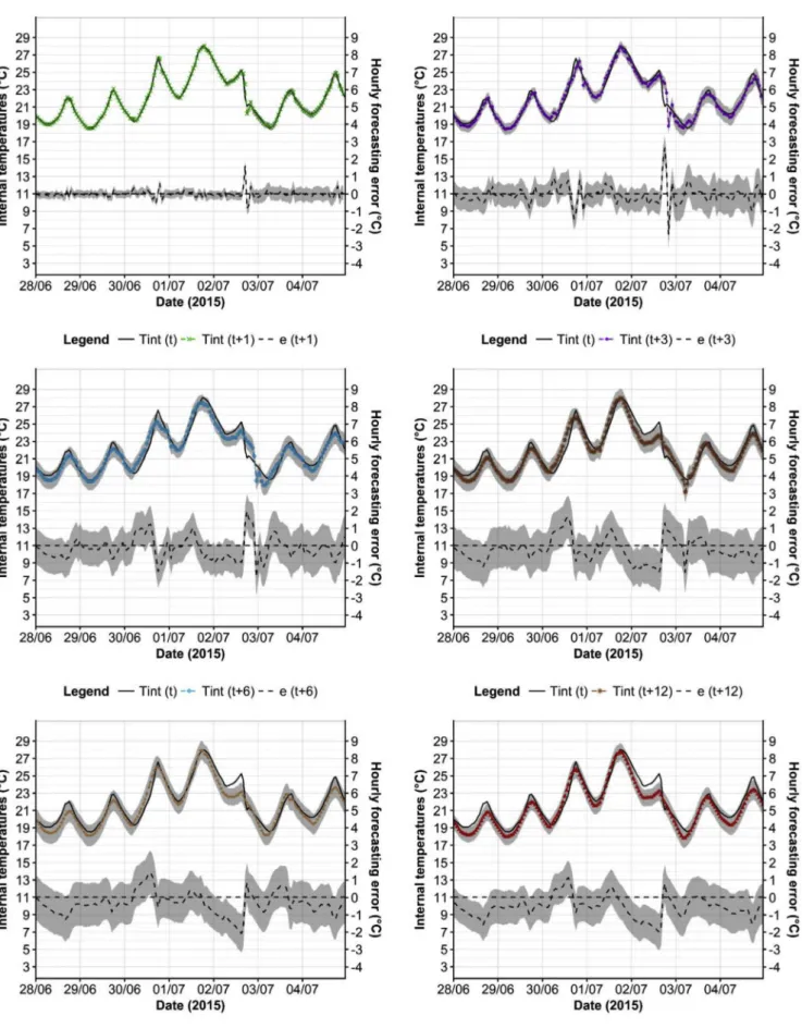
For dwelling B, as for dwelling A, the 1-h forecasts are extremely accurate, with anR2

adjof 0.999. The 3-h, 6-h and 12-h forecasts are also reasonably accurate (Fig. 3). On the other hand, for longer forecasting horizons (24–72 h), the model tends to under-predict the peak tem-perature and struggles to accurately predict the retention of elevated temperatures between the 1stand 2ndJuly. Nonetheless, perhaps be-cause dwelling B has a much smoother internal temperature proﬁle (Fig. 3 cf. Fig. 2), the forecasts are more accurate than those for dwelling A for all the forecasting horizons as measured by theMAEand RMSE(Table 1). The tendency towards under prediction is evident in theMBE. As for dwelling A, the MBE (in absolute terms),MAE and RMSE are all gradually increasing in magnitude as the forecasting horizonhincreases.

2_{Since is not possible to compare the coe}_ffi_{cients for di}_ff_{erent variables} di-rectly, because they are measured on different scales (i.e. unstandardised coefficients), they are expressed as an average percentage weight for each specific input variable:Tint,TextandGHI.

(7)

Fig. 2.Dwelling A: observed,Tint(t), and predicted,Tint(t + h), hourly internal temperatures with hourly forecasting error,e (t + h), and the 95% prediction intervals (grey bands) for 1 h, 3 h, 6 h, 12 h, 24 h and 72 h forecasting horizons,ARXmodel.

(8)

For dwelling C, despite the rapidfluctuations in the measured in-ternal temperature, the model performed with reasonable accuracy throughout the entire week of the heatwave. The unusual temperature profile (i.e. a small increase followed by a sudden fall in the tempera-tures) on the 2nd _{July (}_{Fig. 4}_{) was di}_ffi_{cult for the model to predict} especially at longer forecasting horizons (12–72 h). Despite this chal-lenge, the model performed with comparable accuracy to the model for dwelling A, and with bias and errors that gradually increase with ex-tended forecasting horizons (Table 1).

4.3. Prediction intervals

For all three dwellings, the prediction intervals (grey bands in Figs. 2, 3 and 4) increase as the forecasting horizon (h) increases, with a notable increase from 3 to 6 h. As noted by Hyndman and Athanaso-poulos [38], a common characteristic of prediction intervals is that they tend to gradually increase as the forecasting horizon lengthens. The prediction interval also increases markedly after the heatwave, i.e. 2nd July forh≥6 h, to about ± 1.5 °C and ± 1.25 °C for dwellings A and C respectively, and to approximately ± 0.75 °C for dwelling B.

With two brief exceptions, for all three dwellings and all forecasting horizons up toh= 12, the measured internal temperatures were within the prediction interval. The exceptions were dwellings A and C on 2nd July, where the indoor temperature showed a sudden dramatic de-crease. For prediction horizons h= 24 and h= 72, the internal tem-peratures were not covered by the prediction interval at all times for any of the dwellings on the 1st_{July and, more notably on the 2}nd_July. The observed temperature was above the prediction interval for dwellings B and C, and over then under for dwelling A.

When forecasted temperatures lie outside the prediction interval for a prolonged period it suggests that either the model is not suﬃciently reliable or that the response of the room to changes in ambient con-ditions diﬀers from that which occurred during the training period. These matters are discussed further below.

4.4. Comparison of ARX and ARMAX models

For all three dwellings,ARMAXmodels (q≠0) were developed using the same AutoRegressive and eXogenous terms as in the ARX models (see section 4.1). By varying q, the lowest AIC values were determined as q= 5, q= 4 and q= 6 for dwellings A, B and C re-spectively. Whilst this would suggest that, at least in theory, the ARMAXmodels would provide better forecasting accuracy than ARX models, other aspects need to be considered. Firstly, theAICvalues are determined from the training period for one-step-ahead forecasts only; and secondly, when making actual forecasts, the future residuals cannot be computed a posteriori (and therefore estimates cannot be obtained), and consequently they are set to zero. This means that whilst for one-step-ahead forecasts (h= 1) the model is usingqresiduals in the cal-culation, when 1 <h≤qthe moving average inputs gradually include more zero values, and all are null onceh>q.

Comparison of the predictive accuracy metrics using theARMAX

model (Table 2) with the corresponding accuracy metrics using theARX model (Table 1) indicates that, with proper identiﬁcation of theARX model, theARMAXmodels provide little if any overall improvement. For dwelling A, the ARMAXmodel yielded a lower MBE but at the expense of an increasedRMSEvalue, for dwelling B, theMBEandMAE were very similar but theRMSEwas slightly worse, and for dwelling C, MBE,MAEandRMSEwere all worse for theARMAXmodel for all of the forecasting horizons.

5. Discussion

The aim of this work is to lay the theoretical foundation for an in-home device that could provide an early warning of likely elevated temperatures. Model automation is an extremely important feature of such a device since it obviates the need for manual intervention, trial and error procedures, or model identification by an expert. In principle, therefore, it might be possible to develop a device that needs only a sensor to record the internal zonal air temperature and an internet (or cellular mobile) connection to continuously access and download the weather forecast for a specific location. After an initial training period, the device would be able to automatically select an appropriate model for the specific room before continuing to perform ongoing forecasts of the internal temperatures.

Interestingly, the parameter weightings of the derived models sug-gest that they are relatively immune to the uncertainty in the input weather data. Therefore, even if the derived models were to rely upon forecasted weather data from more distant meteorological stations or on interpolated data (with assumptions about topographical and micro-climate eﬀects), the predictive accuracy may not degrade, which is a useful attribute if the device were deployed in remote locations.

The work undertaken here, concurs with theﬁndings of Mustafaraj et al. [30] in that theARXandARMAXmodels produced similar results, however, as Ríos-Moreno et al. [29] also observed, theARX models were generally a little better overall such that the additional complexity of using anARMAXmodel does not appear to be justiﬁed. The accuracy of theARXpredictions in the rooms that responded more dramatically to external temperature changes (dwellings A and C), are poorer than those reported previously. Ferracuti et al. [33], quoted an RMSEof 0.33 °C for 3-h summertime forecasts in buildings usingARX models, whilst here the values ranged from 0.14 °C in dwelling B, to 0.51 °C and 0.62 °C respectively in dwellings A and C. Likewise, the 2-h summer-time forecasts usingARMAXmodels reported by Mustafaraj et al. [22], produced aMAErange of 0.11–0.19 °C, which is better than the 3-h forecasts for dwellings A and C of 0.35 °C and 0.44 °C, respectively. The results are however, better than those of Ashtiani et al. [32], whose time series regression model was not able to forecast accurately during a heatwave event.

There are several reasons for these differences:firstly, the studies of Mustafaraj et al. [30] and Ferracuti et al. [33] were performed in office buildings with extensive measured data used for the development of the forecasting models. The internal temperatures of offices tend to be less affected by ambient conditions than those in dwellings and individual Table 1

Forecasting accuracy for the week of the 2015 heatwave,ARXmodels.

Forecasting horizonh(hours) Dwelling A Dwelling B Dwelling C

R2

adj(0–1) MBE(°C) MAE(°C) RMSE(°C) R2adj(0–1) MBE(°C) MAE(°C) RMSE(°C) R2adj(0–1) MBE(°C) MAE (°C) RMSE(°C) 1 0.989 −0.02 0.12 0.21 0.999 −0.01 0.04 0.05 0.989 0.01 0.17 0.26 3 0.955 −0.08 0.35 0.51 0.989 −0.03 0.12 0.14 0.910 0.03 0.44 0.62 6 0.921 −0.16 0.51 0.64 0.955 −0.06 0.21 0.24 0.853 0.05 0.55 0.79 12 0.910 −0.24 0.57 0.69 0.910 −0.12 0.28 0.33 0.831 0.08 0.60 0.85 24 0.898 −0.35 0.57 0.71 0.876 −0.20 0.27 0.39 0.819 0.15 0.61 0.86 48 0.887 −0.45 0.62 0.76 0.831 −0.33 0.36 0.46 0.853 0.26 0.59 0.78 72 0.876 −0.56 0.69 0.81 0.729 −0.46 0.49 0.57 0.842 0.31 0.63 0.81

(9)

occupants have less, and sometimes no, personal control over the in-ternal environment. Secondly, the previous work was undertaken during mild summer days with no sudden temperature spikes and peak

indoor temperatures of approximately 24 °C [30] to 26 °C [33]. How-ever, when Mustafaraj et al. used theirARXmodel in a second study [31], in which the internal oﬃce temperatures were higher (28–29 °C) Fig. 3.Dwelling B: observed,Tint(t), and predicted,Tint(t + h), hourly internal temperatures with hourly forecasting error,e (t + h), and the 95% prediction intervals (grey bands) for 1 h, 3 h, 6 h, 12 h, 24 h and 72 h forecasting horizons,ARXmodel.

(10)

Fig. 4.Dwelling C: observed,Tint(t), and predicted,Tint(t + h), hourly internal temperatures with hourly forecasting error,e (t + h), and the 95% prediction intervals (grey bands) for 1 h, 3 h, 6 h, 12 h, 24 h and 72 h forecasting horizons,ARXmodel.

(11)

even though the diurnal range of indoor temperature was similar throughout the week, the MAE of the 2-h predictions increased to 0.37–0.49 °C, which is slightly worse than the 0.12–0.44 °C achieved in this study for 3-h forecasts during a heatwave. Thirdly, in the oﬃce studies of both Mustafaraj et al. and Ferracuti et al. many more inputs were provided to the models than in the work reported here.3

The difficulty that theARX andARMAXmodels, deployed in this study, had in making predictions during abnormal temperature events (and over longer forecasting horizons) is not surprising. Firstly, the models can only be trained based on past events, so the prediction for sudden, rare and more extreme events will always be difficult. Secondly, during such events, the occupants of homes may behave differently; abnormally even. Mitigating actions during a heatwave could include, opening windows and even doors, closing the curtains during the day, turning on portable fans or even using portable air conditioning units. Models learn slowly and so whilst such actions will be incorporated in the model the quality of immediate forward pre-dictions, even for only 3 h ahead will be degraded. Whereas mitigation actions at longer forecasting horizons (3–72 h) might generate occa-sional false positives (i.e. lower temperatures occurred than were pre-dicted, due to the intervening actions taken by the occupants) access to early information regarding the expected room temperatures allows the occupants to take preventive actions. As such, the forecasts can be viewed as a prediction of what will happen if no one intervenes (beyond the established patterns of operation). From a health perspective, this is useful information since it allows the occupants (or their carers) to take action to lower the indoor temperatures in order to contain them within a comfort range or within acceptable heat-stress levels. Because at shorter forecasting horizons (1–3 h) the predictions are considerably more accurate and consistent, and because the target ambulance re-sponse times in the UK for non-urgent calls are within 3 h for 90% of the calls [50], a warning device could be set to dispatch the emergency services in advance in order to reach vulnerable occupants (i.e. those most at risk during hot weather) in a timely manner. Additional sensors, for example to detect window opening or internal air velocities, could assist the model, but this adds cost and complexity and only deals with one of the many possible occupant responses.

Future work will focus initially on further improvements to the modelling procedure and understanding the factors that aﬀect the models' predictive accuracy. One approach that will be explored is the use of non-linear models (e.g.ANNmodels etc.), which were shown in the study by Mustafaraj et al. [31] to produce more accurate forecasts than linearARXmodels. In addition, the models will be tested on da-tasets that contain information on window opening patterns in order to examine their eﬀect on the predictions of the models.

This work has examined three, speciﬁcally-selected rooms, in

diﬀerent dwellings located in the same town, with hourly temperatures recorded over just one summer period. Future endeavours will entail testing the modelling process and quantifying the models' accuracy, for many more rooms, households, dwelling types and locations.

Ultimately, it is hoped that forecasts of suﬃcient reliability could be provided to vulnerable occupants (and their carers) several days in advance (24–72 h) with minimal monitoring and at a low cost. This would allow occupants, carers and perhaps the emergency services adequate time to prepare for an impending response. Whilst the very reliable short-term forecasts (1–12 h) would allow the targeted de-ployment and triaging of emergency services.

6. Conclusions

The potential for statistical models to predict indoor temperatures during heatwaves has been investigated using hourly data from three bedrooms, in three houses, located close to the town of Loughborough in the UK Midlands. During the monitoring period, there was a two-day heatwave during which the external dry-bulb temperature exceeded 35 °C. TheAIC was adopted to automatically identify a near optimal forecasting model, specific to each room, using data from before the period of hot weather. Recursive multi-step-ahead forecasts were made by bothARX andARMAXmodels using a rolling forecasting origin. These provided predictions for forecasting horizons of 1, 3, 6, 12, 24 and 72 h for the whole week of the heatwave. The accuracy of the predictions over that week were evaluated using theMBEandR2adjas measures of the bias and out-of-samplefit of the models, andMAEand RMSEto assess the forecasting accuracy of the models. The 95% pre-diction intervals were computed for the heatwave week to express the reliability of the forecasts at different forecasting horizons.

Comparison between the ARX and ARMAX models showed that whilst they produce almost identical one-step-ahead forecasts when longer multi-step-ahead forecasts are performed, with a recursive strategy, theARXmodels were simpler to derive and oﬀered slightly more consistent, reliable and accurate predictions. The ARX models produced anMAEbelow 0.7 °C during a heatwave week for all three dwellings and for all of the forecasting horizons up to 72 h. The internal temperatures tended to be under-predicted for two dwellings,MBEup to−0.56 °C, but over-predicted for the other,MBE, 0.31 °C. The range of the 95% prediction interval varied from ± 0.75 °C in one dwelling to ± 1.50 °C in the dwellings that responded more dramatically to the elevated temperatures during the heatwave. With very limited local exceptions, the actual temperatures were within the prediction interval for all forecasting horizons up to 12 h.

Overall the earlyﬁndings of the work reported here suggest that highly detailed building information is not required to produce rea-sonable forecasts of indoor temperatures in free-running (i.e. without mechanical cooling and heating) dwellings.

This points to the potential for using time series forecasting as part of an overheating early-warning system in buildings, especially those housing vulnerable occupants or contents. Future work will explore alternative non-linear modelling approaches and examine the eﬀect of Table 2

Forecasting accuracy for the week of the 2015 heatwave,ARMAXmodels.

Forecasting horizonh(hours) Dwelling A Dwelling B Dwelling C

R2

adj(0–1) MBE(°C) MAE(°C) RMSE(°C) R2adj(0–1) MBE(°C) MAE(°C) RMSE(°C) R2adj(0–1) MBE(°C) MAE(°C) RMSE(°C) 1 0.989 0.00 0.17 0.26 0.999 −0.01 0.04 0.05 0.989 −0.02 0.12 0.21 3 0.865 0.01 0.56 0.75 0.977 −0.04 0.14 0.16 0.932 −0.14 0.43 0.62 6 0.797 0.00 0.70 0.94 0.932 −0.10 0.24 0.28 0.786 −0.40 0.80 1.05 12 0.786 0.00 0.70 0.96 0.898 −0.15 0.30 0.36 0.865 −0.36 0.67 0.86 24 0.774 0.11 0.67 0.98 0.842 −0.25 0.31 0.45 0.887 −0.45 0.64 0.78 48 0.831 0.20 0.61 0.85 0.774 −0.38 0.42 0.53 0.865 −0.58 0.71 0.85 72 0.842 0.23 0.59 0.81 0.684 −0.45 0.51 0.62 0.831 −0.70 0.79 0.94

3_{Mustafaraj et al. [}₃₀_,₃₁_{]: internal and external temperatures; internal and} external relative humidity; supply airﬂow-rate, air temperature and relative humidity of the air handling units; chilled water temperature of the chillers; hot waterﬂow temperature to the fan coil unit. Ferracuti et al. [33]: internal and external temperatures, solar gains, internal gains and thermal gains.

(12)

windows opening and other occupant interventions on the predictive accuracy of the models. Finally, testing of the prototype forecasting models on larger datasets will be carried out in order to quantify the reliability of predictions for diﬀerent rooms, dwelling and household conﬁgurations across a wide range of geographic locations.

Declarations of interest

None.

Acknowledgements

This research was made possible by Engineering and Physical Sciences Research Council (EPSRC) support for the London-Loughborough (LoLo) Centre for Doctoral Training in Energy Demand (grant EP/L01517X/1). Monitored data, indispensable to this study, was made available by the open access REFIT Smart Home dataset [34], which was funded by the EPSRC:‘REFIT: Personalised Retroﬁt Decision Support Tools for UK Homes using Smart Home Technology’(grant EP/ K002457/1).

Nomenclature

αn eXogenous coeﬃcient (weight) of the past/forecasted ex-ternal air Temperature (Text) at lagn

AIC Akaike Information Criterion ADF test Augmented Dickey-Fuller test

ARIMAX (p, d, q, x) AutoRegressive Integrated Moving Average with eXogenous inputs

ARMAX (p, q, x) AutoRegressive Moving Average time series with eXogenous inputs (d = 0)

ANN Artiﬁcial Neural Network

ARX (p, x) AutoRegressive time series with eXogenous inputs (d = 0; q = 0)

BIC Bayesian Information Criterion

βn eXogenous coeﬃcient (weight) of the past/forecasted Global Horizontal Irradiance (GHI) at lagn

c intercept (regression constant) [°C]

γq Moving Average coeﬃcient (weight) of the past residual at lagq

d integration order: adopted order of diﬀerencing required to make the input data stationary

e (t+h - q) residuals: the hourly diﬀerence between the observed and forecasted internal temperatures at the time step t for the forecasting horizonhand lagq[°C]

e (t+h) forecasting error: the hourly diﬀerence between the fore-casted and observed internal temperatures at the time stept for the forecasting horizonh[°C]

GHI observed or forecasted hourly Global Horizontal Irradiance [W/m2]

h forecasting horizon (h-step forecast) [h]

k coverage factor (k= 1.96 standard deviations for the 95% prediction interval)

ℒ maximimum likelihood of the estimated model MAE Mean Absolute Error [°C]

MBE Mean Bias Error [°C]

n lag (nthprevious time step of the input variable) [h] N number of estimated parameters in the model

p AutoRegressive inputs: number of past observed values con-sidered as predictors

ϕn AutoRegressive coeﬃcient (weight) of the past internal Temperature (Tint) at lagn

PIh 95% prediction interval for the forecasting horizonh[°C] q Moving Average (MA) order: number of past residuals

con-sidered as predictors

R2adj adjusted coeﬃcient of determination [0–1]

RMSE Root Mean Squared Error [°C]

σh the standard deviation of theh-step forecast distribution t hourly time step [h]

Text observed or forecasted hourly external air Temperature [°C] Tint(t) observed hourly internal Temperature at the time stept[°C] Tint(t+h) forecasted hourly internal Temperature at the time stept

for the forecasting horizonh[°C]

x eXogenous inputs: number of external variables adopted as predictors

References

[1] NHBC, Overheating in new homes; A review of the evidence, (2012),http://www. zerocarbonhub.org/sites/default/ﬁles/resources/reports/Overheating_in_New_ Homes-A_review_of_the_evidence_NF46.pdf.

[2] ZCH, Overheating in homes - The big picture, (2016),http://www.zerocarbonhub. org/sites/default/ﬁ

les/resources/reports/ZCH-OverheatingInHomes-TheBigPicture-01.1.pdf.

[3] K.J. Lomas, S.M. Porritt, Overheating in buildings: lessons from research, Build. Res. Inf. (2017) 1–18,https://doi.org/10.1080/09613218.2017.1256136. [4] G.A. Meehl, C. Tebaldi, More intense, more frequent, and longer lasting heat waves

in the 21st century, Science 305 (2004) 994–997,https://doi.org/10.1126/science. 1098704, (80-. ).

[5] IPCC, Climate change 2014, Synth.Rep. (2014),https://doi.org/10.1017/ CBO9781107415324.

[6] G.J. Jenkins, M.C. Perry, M.J. Prior, The Climate of the UK and Recent Trends, Met Oﬃce Hadley Centre, Exeter, UK, 2009,http://ukclimateprojections.defra.gov.uk/ images/stories/trends_pdfs/Trends.pdf.

[7] G.S. Jones, P.A. Stott, N. Christidis, Human contribution to rapidly increasing fre-quency of very warm Northern Hemisphere summers, J. Geophys. Res. Atmos. 113 (2008) 1–17,https://doi.org/10.1029/2007JD008914.

[8] Public Health England, Heatwave plan for England: protecting health and reducing harm from severe heat and heatwaves, London,https://www.gov.uk/government/ uploads/system/uploads/attachment_data/ﬁle/429384/Heatwave_Main_Plan_ 2015.pdf, (2015).

[9] A. De Bono, G. Giuliani, S. Kluster, P. Peduzzi, Impacts of summer 2003 heat wave in Europe, Environ. Alert Bull. UNEP (2004) 4,https://doi.org/10.1017/ S0147547903000218.

[10] G.P. Kenny, J. Yardley, C. Brown, R.J. Sigal, O. Jay, Heat stress in older individuals and patients with common chronic diseases, CMAJ (Can. Med. Assoc. J.) 182 (2010) 1053–1060,https://doi.org/10.1503/cmaj.081050.

[11] S. Hajat, R.S. Kovats, K. Lachowycz, Heat-related and cold-related deaths in England and Wales: who is at risk? Occup. Environ. Med. 64 (2007) 93–100,

https://doi.org/10.1136/oem.2006.029017.

[12] Age UK, Later Life in the United Kingdom, (2018),https://www.ageuk.org.uk/ Documents/EN-GB/Factsheets/Later_Life_UK_factsheet.pdf?dtrk=true.

[13] J. Cui, A. Arbab-Zadeh, A. Prasad, S. Durand, B.D. Levine, C.G. Crandall, Eﬀects of heat stress on thermoregulatory responses in congestive heart failure patients, Circulation 112 (2005) 2286–2292,https://doi.org/10.1161/CIRCULATIONAHA. 105.540773.

[14] W. Huang, H. Kan, S. Kovats, The impact of the 2003 heat wave on mortality in Shanghai, China, Sci. Total Environ. 408 (2010) 2418–2420,https://doi.org/10. 1016/j.scitotenv.2010.02.009.

[15] C. Rooney, A.J. McMichael, R.S. Kovats, M.P. Coleman, Excess mortality in England and Wales, and in Greater London, during the 1995 heatwave, J. Epidemiol. Community Health 52 (1998) 482–486,https://doi.org/10.1136/jech.52.8.482. [16] S.N. Gosling, J.A. Lowe, G.R. McGregor, M. Pelling, B.D. Malamud, Associations between Elevated Atmospheric Temperature and Human Mortality: a Critical Review of the Literature, (2009),https://doi.org/10.1007/s10584-008-9441-x. [17] M. Anderson, C. Carmichael, V. Murray, A. Dengel, M. Swainson, Deﬁning indoor

heat thresholds for health in the UK, Perspect. Public Health 133 (2013) 158–164,

https://doi.org/10.1177/1757913912453411.

[18] B.G. Armstrong, Z. Chalabi, B. Fenn, S. Hajat, A. Milojevic, P. Wilkinson, The as-sociation of mortality with high temperatures in a temperate climate : England and Wales, J. Epidemiol. Community Health 65 (2010) 340,https://doi.org/10.1136/ jech.2009.093161.

[19] S.H. Holmes, T. Phillips, A. Wilson, Overheating and passive habitability: indoor health and heat indices, Build. Res. Inf. 44 (2016) 1–19,https://doi.org/10.1080/ 09613218.2015.1033875.

[20] R. Basu, J.M. Samet, An exposure assessment study of ambient heat exposure in an elderly population in Baltimore, Maryland, Environ. Health Perspect. 110 (2002) 1219–1224,https://doi.org/10.1289/ehp.021101219.

[21] K. Lomas, T. Kane, Summertime temperatures and thermal comfort in UK homes, Build. Res. Inf. 41 (2013) 259–280,https://doi.org/10.1080/09613218.2013. 757886.

[22] A. Beizaee, K.J. Lomas, S.K. Firth, National survey of summertime temperatures and overheating risk in English homes, Build. Environ. 65 (2013) 1–17,https://doi.org/ 10.1016/j.buildenv.2013.03.011.

[23] A. Mavrogianni, A. Pathan, E. Oikonomou, P. Biddulph, M. Davies, A. Mavrogianni, A. Pathan, E. Oikonomou, P. Biddulph, Inhabitant actions and summer overheating risk in London dwellings, Build. Res. Inf. 0 (2016) 1–24,https://doi.org/10.1080/ 09613218.2016.1208431.

(13)

[24] R. McLeod, M. Swainson, Chronic overheating in low carbon urban developments in a temperate climate, Renew. Sustain. Energy Rev. 74 (2017) 201–220,https://doi. org/10.1016/j.rser.2016.09.106.

[25] S.M. Porritt, P.C. Cropper, L. Shao, C.I. Goodier, Ranking of interventions to reduce dwelling overheating during heat waves, Energy Build. 55 (2012) 16–27,https:// doi.org/10.1016/j.enbuild.2012.01.043.

[26] R. McLeod, C. Hopfe, Y. Rezgui, A proposed method for generating high resolution current and future climate data for Passivhaus design, Energy Build. 55 (2012) 481–493,http://dx.doi.org/10.1016/j.enbuild.2012.08.045.

[27] R. McLeod, C. Hopfe, A. Kwan, An investigation into future performance and overheating risks in Passivhaus dwellings, Build. Environ. 70 (2013) 189–209,

https://doi.org/10.1016/j.buildenv.2013.08.024.

[28] P. Symonds, J. Taylor, A. Mavrogianni, M. Davies, C. Shrubsole, I. Hamilton, Z. Chalabi, Overheating in English dwellings: comparing modelled and monitored large-scale datasets, Build. Res. Inf. 45 (2016) 195–208,https://doi.org/10.1080/ 09613218.2016.1224675.

[29] G.J. Ríos-Moreno, M. Trejo-Perea, R. Castañeda-Miranda, V.M. Hernández-Guzmán, G. Herrera-Ruiz, Modelling temperature in intelligent buildings by means of auto-regressive models, Autom. ConStruct. 16 (2007) 713–722,https://doi.org/10. 1016/j.autcon.2006.11.003.

[30] G. Mustafaraj, J. Chen, G. Lowry, Development of room temperature and relative humidity linear parametric models for an open oﬃce using BMS data, Energy Build. 42 (2010) 348–356,https://doi.org/10.1016/j.enbuild.2009.10.001.

[31] G. Mustafaraj, G. Lowry, J. Chen, Prediction of room temperature and relative humidity by autoregressive linear and nonlinear neural network models for an open oﬃce, Energy Build. 43 (2011) 1452–1460,https://doi.org/10.1016/j.enbuild. 2011.02.007.

[32] A. Ashtiani, P.A. Mirzaei, F. Haghighat, Indoor thermal condition in urban heat island: comparison of the artiﬁcial neural network and regression methods pre-diction, Energy Build. 76 (2014) 597–604,https://doi.org/10.1016/j.enbuild.2014. 03.018.

[33] F. Ferracuti, A. Fonti, L. Ciabattoni, S. Pizzuti, A. Arteconi, L. Helsen, G. Comodi, Data-driven models for short-term thermal behaviour prediction in real buildings, Appl. Energy 204 (2017) 1375–1387,https://doi.org/10.1016/j.apenergy.2017.05. 015.

[34] S. Firth, T. Kane, V. Dimitriou, T. Hassan, F. Fouchal, M. Coleman, L. Webb, REFIT Smart Home Dataset, (2016),https://doi.org/10.17028/rd.lboro.2070091. [35] F. Amara, K. Agbossou, A. Cardenas, Y. Dubé, S. Kelouwani, Comparison and

simulation of building thermal models for eﬀective energy management, Smart Grid Renew. Energy 6 (2015) 95–112,https://doi.org/10.4236/sgre.2015.64009. [36] A. Foucquier, S. Robert, F. Suard, L. Stéphan, A. Jay, State of the art in building

modelling and energy performances prediction: a review, Renew. Sustain. Energy Rev. 23 (2013) 272–288,https://doi.org/10.1016/j.rser.2013.03.004. [37] R. Kramer, J. van Schijndel, H. Schellen, Simpliﬁed thermal and hygric building

models: a literature review, Front. Archit. Res. 1 (2012) 318–325,https://doi.org/ 10.1016/j.foar.2012.09.001.

[38] J.R. Hyndman, G. Athanasopoulos, Forecasting: Principles and Practice, second ed., OTexts, 2018, ISBN-13: 978-0987507112.

[39] R. Chandra, Y.S. Ong, C.K. Goh, Co-evolutionary multi-task learning with predictive recurrence for multi-step chaotic time series prediction, Neurocomputing 243 (2017) 21–34,https://doi.org/10.1016/j.neucom.2017.02.065.

[40] S. Ben Taieb, R.J. Hyndman, Recursive and Direct Multi-step Forecasting: the Best of Both Worlds, (2012), issn: 1440–1771X.

[41] K. Judd, M. Small, Towards long-term prediction, Phys. D 136 (2000) 31–44,

https://doi.org/10.1016/S0167-2789(99)00152-9.

[42] F.J. Chang, Y.M. Chiang, L.C. Chang, Multi-step-ahead neural networks forﬂood forecasting, Hydrol. Sci. J. 52 (2007) 114–130,https://doi.org/10.1623/hysj.52.1. 114.

[43] Met Oﬃce, Heatwave,https://www.metoﬃce.gov.uk/learning/temperature/ heatwave, (2018), Accessed date: 16 July 2018.

[44] WMO, Guidelines on the deﬁntion and monitoring of extreme weather and climate events, World Meteorol. Organ (2016) 62.

[45] Met Office, Heatwave 1 July 2015-Met Office, (2015),http://www.metoffice.gov. uk/climate/uk/interesting/july2015, Accessed date: 12 September 2017. [46] S. Makridakis, C.S. Wheelwright, J.R. Hyndman, Forecasting: Methods and

Applications, third ed., John Wiley & Sons, Inc., 1998, ISBN-13:13978-0-471-53233-0.

[47] G. Shmueli, To explain or to predict? Stat. Sci. 25 (2010) 289–310,https://doi.org/ 10.1214/10-STS330.

[48] R: The R Project for Statistical Computing, (n.d.),https://www.r-project.org/, Accessed date: 27 March 2018.

[49] Met Office, 10 day weather forecast - Met Office, (2016),https://www.metoffice. gov.uk/guide/weather/10-day-forecast, Accessed date: 27 November 2017. [50] NHS, NHS England - New ambulance standards, (2017),https://www.england.nhs.