Text Filtering and Ranking for Security Bug
Report Prediction
Fayola Peters, Thein Than Tun,
Member, IEEE,
Yijun Yu,
Member, IEEE,
and Bashar Nuseibeh,
Member, IEEE
Abstract—Security bug reports can describe security critical vulnerabilities in software products. Bug tracking systems may contain thousands of bug reports, where relatively few of them are security related. Therefore finding unlabelled security bugs among them can be challenging. To help security engineers identify these reports quickly and accurately, text-based prediction models have been proposed. These can often mislabel security bug reports due to a number of reasons such as class imbalance, where the ratio of non-security to security bug reports is very high. More critically, we have observed that the presence of security related keywords in both security and non-security bug reports can lead to the mislabelling of security bug reports. This paper proposes FARSEC, a framework for filtering and ranking bug reports for reducing the presence of security related keywords. Before building prediction models, our framework identifies and removes non-security bug reports with security related keywords. We demonstrate that FARSEC improves the performance of text-based prediction models for security bug reports in 90% of cases. Specifically, we evaluate it with 45,940 bug reports from Chromium and four Apache projects. With our framework, we mitigate the class imbalance issue and reduce the number of mislabelled security bug reports by 38%.
Index Terms—security cross words, security related keywords, security bug reports, text filtering, ranking, prediction models, transfer learning.
F
1
I
NTRODUCTIONBug tracking systems help developers maintain software products by allowing reporters to submit any bugs en-countered while using these software products. Some bug reports can describe security vulnerabilities which could be exploited by attackers if they are exposed before they are fixed. A security bug is a security vulnerability that allows a user to have inappropriate access to the system and thus cause harm or damage to the software or to persons using the software [1]. Vendors usually request that bug reporters do not disclose any suspected security vulnerabilities in public bug tracking systems. Instead, they suggest that suspected security vulnerabilities be reported directly and privately to security engineers who assess them and, when necessary, provide patches to customers before an attacker discovers and exploits the vulnerability. Once a patch has been disseminated, vulnerabilities are often documented and disclosed via the bug tracking system [2].
In reality, because of the lack of security domain knowl-edge on the part of some bug reporters [3], or others who simply ignore the request from vendors and security engineers, suspected security bug reports are often publicly disclosed before they are assessed and fixed [4]. To help security engineers identify security bug reports quickly and accurately, text-based prediction models have been proposed, and implemented in industry [1], [3], [4]. These prediction models are a combination of labelled bug reports
• F. Peters and B. Nuseibeh are with Lero - The Irish Software Research Centre, University of Limerick, Limerick, Ireland.
E-mail:{fayola.peters, bashar.nuseibeh}@lero.ie
• T. T. Tun, Y. Yu and B. Nuseibeh are with the Department of Computing and Communications, The Open University, Milton Keynes, United Kingdom.
E-mail:{thein.tun, yijun.yu, bashar.nuseibeh}@open.ac.uk
and machine learning algorithms. However, there is one underlying issue not fully explored in these models, which we callsecurity cross words. Security cross words denotethe use of the same security related keywords in both security and
non-security bug reports. We have observed that text-based prediction models can mislabel security bug reports when security cross words are present. The problem is magnified if there is class imbalance where non-security bug reports outnumber security bug reports by a large margin. For instance, among the 45,940 bug reports studied in this paper, only 0.8% are known to be security bug reports.
We propose FARSEC, a framework composed of a combi-nation of Filtering And Ranking methods to reduce the misla-belling ofSECurity bug reports by text-based prediction models.
When building prediction models, FARSEC automatically identifies and removes non-security bug reports containing security cross words. It begins by finding security related keywords from the security bug reports of a project (Sec-tion 3.1). Each security related keyword isscoredaccording to its frequency in both security and non-security reports. Using the keyword scores of bug reports, we remove non-security reports with scores as high as those of non-security bug reports (Section 3.2). The remaining bug reports are used to build prediction models (Section 3.3). Finally, FARSEC uses the results of the prediction models to present security engineers with ranked lists of bug reports where most of the actual security bug reports are closer to the top of the ranked lists than at the bottom.
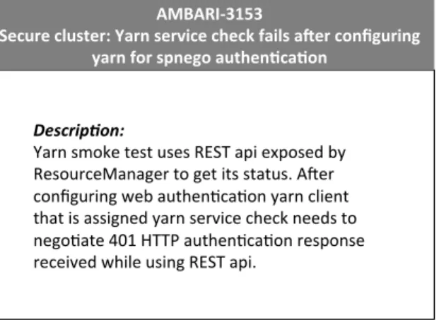
To illustrate how FARSEC works, consider the exam-ple in Figure 1. When the data was downloaded on May 5th, 2017, the report was labelled as a non-security bug report (NSBR) by researchers (see Section 4.1). However, in the official bug tracking system of the Ambari project,
JOURNAL OF LATEX CLASS FILES, VOL. 14, NO. 8, AUGUST 2015 2
Descrip(on:
Yarn smoke test uses REST api exposed by ResourceManager to get its status. A<er configuring web authen@ca@on yarn client that is assigned yarn service check needs to nego@ate 401 HTTP authen@ca@on response received while using REST api.
AMBARI-3153
Secure cluster: Yarn service check fails a<er configuring yarn for spnego authenBcaBon
configuring yarn for spnego authen@ca@on.
Fig. 1.Ambari-3153is a bug report mislabelled as non-security.
Ambari-3153 was described as a security bug report (SBR)1. Such mislabelling of security reports could not only
lead to the exploitation of the particular vulnerability in-volved, but also make prediction models based on this data to mislabel future SBRs. Filtering and ranking capabilities of FARSEC would remove reports such asAmbari-3153from its training data.
We evaluate FARSEC with a total of 41,940 bug reports from Chromium and four Apache projects (Section 4.1) each containing 1000 reports. We also use five machine learning algorithms (Section 4.3) and six performance measures (Sec-tion 4.4) to evaluate our approach. We then consider the following research questions:
RQ1: Can security cross words lead to mislabelled secu-rity bug reports by prediction models?
We look at the number of security cross words present before and after using FARSEC. We then consider these numbers in conjunction with the pre-diction of SBRs using prepre-diction models. The results indicate that security cross words can contribute to mislabelled SBRs (Section 5.1).
RQ2: How do we build effective prediction models for security bug reports when data scarcity is an issue? To build effective prediction models we need suffi-cientdata from both security and non-security bug reports. When data scarcity is an issue, one solution is to use data from other projects to build prediction models. Results show better performance in favour of using FARSEC and data from other projects (Sec-tion 5.2).
RQ3: How do we generate useful lists of ranked bug reports?
FARSEC produces ranked lists of bug reports. We view the usefulness of the ranked lists as having more actual SBRs at the top of the lists than at the bottom. Our results show that for all the projects, FARSEC lists are more useful than non-FARSEC lists (Section 5.3).
FARSEC is a framework designed to reduce the mis-labelling of security bug reports by text-based prediction models. It makes the following contributions:
1. https://issues.apache.org/jira/browse/AMBARI-3153
1) An approach to automatically identify security re-lated keywords and security cross words from secu-rity bug reports.
2) An automatic filtering and ranking method to build better text-based prediction models for security bug reports by removing NSBRs with security cross words from the prediction model. Better prediction models reduce the mislabelling of security bug re-ports.
3) A tractable method to use both bug reports from within a single project and bug reports from other projects to build text-based prediction models for security bug reports.
4) A ranking capability used to generate a useful ranked list of bug reports where most of the actual security bug reports are closer to the top of the list.
2
B
ACKGROUND ANDR
ELATEDW
ORKExisting research has proposed prediction models to detect security vulnerabilities in both the pre- and post-release phases of software development. In the pre-release phase the source code is used to build prediction models [5]–[10] while bug reports are used in the post-release phase [1], [3], [4]. Although the data used in these phases are different, the process for building the prediction models face the same issues of class imbalance, cross words, and insufficient data. 2.1 Security Vulnerability Models with Source Code Source code can be used to derive metric-based and text-based prediction models. Metric-text-based models are fash-ioned after defect prediction models. Similarly, they use code metrics such as code churn, complexity, coupling and cohesion metrics, and code coverage [5]–[7], [9], [10]. Zimmermannet al. [5] and Shin et al. [6], [7] investigated the feasibility of these metrics (classical metrics) for security vulnerability prediction. The former performed their study on Windows Vista and found that the metrics had a low correlation with vulnerabilities and could predict them with good precision but with very low recall. In addition they found that the use of dependencies for prediction worked better than the code metrics in terms of better recall.
Studies by Shinet al. were done on open source projects, namely the Mozilla Firefox web browser and the Red Hat Enterprise Linux kernel. Out of 28 metrics, 24 were dis-criminative for security vulnerabilities in both projects [6]. Later they found that their vulnerability prediction model from Mozilla had a recall of 83% and precision of 12% at a classification threshold 0.5 [7].
Text-based models use terms and their frequencies in source code to build prediction models for security vulner-abilities. In their study of 20 android applications, Scandari-atoet al. [8] used text-based models to predict vulnerabil-ities in software components. Walden et al. [9] compared metric-based models with text-based models for source code and found that the text-based models performed best with higher recall in three web applications.
Class imbalance affects the performance of machine learning algorithms in the presence of under-represented data and severe class distribution skews [11]. A study by
Morrisonet al. [10] has noted that while Microsoft product teams have adopted defect prediction models, they have not adopted vulnerability prediction models. This was due to their poor performance in terms of precision and recall with highly imbalanced data.
In this paper we focus on security vulnerability pre-dictors built with bug reports (described in the following section). We face the same issue of class imbalance where out of the 45,940 bug reports studied, only 0.8% are security bug reports.
2.2 Security Vulnerability Models with Bug Reports Building security vulnerability models with the natural lan-guage text of bug reports is a text-mining task. First, relevant keywords are identified with semi-automatic methods and then prediction models are built using these as a feature set along with their frequencies in each document. An early work on this topic by Gegicket al. [3] highlighted the prob-lem of SBRs being mislabelled as NSBRs because of (say) the lack of security domain knowledge of bug reporters. Their research resulted in an approach that leveraged the natural language descriptions of bug reports to train a statistical model in an effort to identify SBRs that were manually mislabelled as NSBRs. Security engineers could use their model to automate the classification of bugs. Their evalua-tion was based on a proprietary software system from Cisco. In this paper our evaluations are done with open source data (Table 1), allowing our experiments to be reproducible.
Later research by Wijayasekara et al. [4] focused on the problem of hidden impact vulnerabilities where security bug reports are only identified after being made public. In an analysis they revealed that among the discovered vul-nerabilities in the Linux kernel and MySQL, 32% and 62% respectively were hidden impact vulnerabilities. They also showed that these values increased in the following years. The authors proposed a vulnerability discovery methodol-ogy where they distinguished between long and short bug reports prior to applying text-mining methods. A base-rate fallacy evaluation was used to acknowledge the issue of class imbalance. This measure allows security engineers to choose prediction models based on the false positive alarm rates they would be willing to accept. For example, if a prediction model has a precision of 0.01, it means that out of 100 predicted SBRs, one will be an actual SBR.
2.2.1 Methods for Finding Security Related Keywords For many researchers, identifying security related keywords usually starts with a seed list which is expanded semi-automatically using external sources. For instance Gegick
et al. [3] mentioned in their configuration file preparation phase that they obtained terms from bug reports to pop-ulate start, stop and synonym keyword lists. The authors described manually adding terms such asvulnerabilityand
attackfrom security bug reports to start lists. Also included were terms, which were not explicitly security related, such ascrashandexcessive. In a similar vein, Pleteaet al. [12] used an iterative process to construct a set of security relevant keywords, which they called akeyword-basedapproach. They started with a seed list derived from the existing literature and their own security expertise. Their seed list contained
keywords such assecurity,ssl,encryptionandauthentication, which is expanded using co-occurring tags from Stack Over-flow.
In the analysis of software maintenance techniques, Hin-dle et al. [13] created three keyword lists using external sources independent of the data used in their study. Using an ontology for software quality measurement and the ISO9126 taxonomy 2, they associated keyword lists with
six labels from the standard for non-functional requirements (namely, maintainability, functionality, portability, efficiency, usability, and reliability). One of the labels is functionality, to which security is associated. Hindleet al. [13] then expanded the keyword lists using WordNet and a random analysis of mailing list messages from an open source project, where any word considered to be associated with a non-functional requirement is added to the keyword list. In this paper we automatically identify security related keywords using the text in SBRs and tf-idf (Section 3.1), and without using external sources. Nevertheless, many of our keywords are similar to those found in other studies [3], [12], [13]. 2.2.2 Transfer Learning and Prediction Models
One fundamental assumption of traditional machine learn-ing algorithms is that the trainlearn-ing (past) data and present (test) data have the same features and distribution. This assumption does not hold, for example, when the training data and present data come from different projects.Transfer learningaims to bridge this gap by extracting useful knowl-edge from past data and applying it to different present data. This is especially useful when the target data is new and has not been examined by domain experts [14].
Following defect prediction models, some vulnerability prediction approaches use code metrics. One line of re-search on defect prediction is cross project defect prediction (CPDP), which uses data from external sources to build models [15]. CPDP is useful because for many companies that are relatively small or have new products, local data may not be readily available. With the use of better selection tools for training data and transfer learning techniques, researchers found it possible to predict defects for “data starved” software projects by using data from external sources [16]–[24].
Results from existing studies of SBRs are currently incon-clusive [3], [8]. The ability to use data from other sources to predict security bugs has been studied with mixed results. For example, Gegicket al. [3] recommended that the trained model should not be applied to software systems in which the SBRs describe different types of security bugs than those that were used to train the model [3]. On the other hand, Scandariato et al. [8] found that some models built on a single application can predict which software components are vulnerable in other applications. However, they admit that they do not have a technique to identify which appli-cations have data that can be used to produce the general vulnerability prediction models.
Chawlaet al. [1], used tf-idf (a statistic for weighting key-words described in Section 3.1) and the semantic similarity of the keywords found with tf-idf in order to generate their
2. ISO/IEC 25010:2011 has recently added “security” as one of the main characteristics of software qualities.
1. Tokenize SBRs
2. Keep Top Tf-idf Terms
3. Make Train Data Matrix*
with Top Terms
Iden&fy Security
Related Keywords Filtering 1. Score Terms
2. Score Bug Reports
3. Remove NSBRs with high Scores
Make Test Data Matrix with Top Terms
Ranking 1. Sort by Report
PredicGon
1 2 3
Scoring and PredicGon of Test Data Matrix
*In a Data Matrix each row represents a bug report. SBR PredicGon
Model
Train
Test
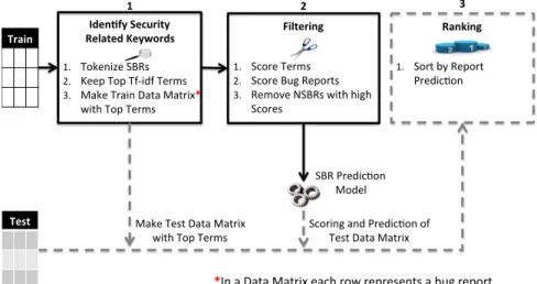
Fig. 2. Overview of the FARSEC approach
keyword lists. Their Multinomial Naive Bayes predictor was able to label bug reports as security, regression, polish and cleanup. Similarly, they used Chromium bug reports in their evaluation and hinted at (security) cross words when they described manually removing keywords from the four different categories of Chromium, which appeared in the top 50 keywords of each category. Their intuition was that these keywords did not seem to provide a discriminative contribution. In this paper we automatically identify secu-rity cross words, but we do not remove all of them from our feature set because at least 74% of the security related keywords identified in our study are cross words. Instead we use them to remove NSBRs from the data sets in order to improve the prediction of SBRs.
To conclude, this paper proposes a novel method for constructing text-based prediction models for security bug reports, focusing on the issue of security cross words. Our results show that appropriately dealing with security cross words provides a foundation for dealing with other issues such as insufficient data, feature selection and class imbal-ance.
3
FARSEC D
ESIGN ANDO
PERATIONWith FARSEC, our goal is to improve text-based prediction models for SBRs. When building prediction models, FAR-SEC automatically identifies and removes NSBRs containing security cross words. Figure 2 shows the three main stages of FARSEC: 1) identifyingsecurity related keywords(Section 3.1); 2) filtering via the scoring of security related keywords and bug reports (Section 3.2); and 3) ranking based successive sorting and prediction (Section 3.3). The result is a sorted list of predicted bug reports where most, if not all, SBRs are expected to appear above NSBRs.
3.1 Identifying Security Related Keywords
To identify security related keywords and security cross words from bug reports, we first tokenize the SBRs and then calculate the tf-idf values of each term (explained in Step 4 below). We consider the hundred terms with the highest tf-idf values to be security related keywords. Of these 100
terms, we consider those found in NSBRs to be security cross words. The security related keywords are then used to build term-document matrices using the following steps (keywordsandtermsare used interchangeably):
1) Tokenize text: This is a frequently used method in text mining, which involves splitting text into sentences and words [25]. In addition, it is common to extract token features that are usually categorical functions of tokens such as types of capitalization, punctuation and special characters [25]. As part of tokenizing text in this paper, we make all terms lowercase.
2) Removestop words: Stop words are common words that are irrelevant to the classification task [25] and are therefore removed. Some examples of En-glish stop words include: a, again, on, the, their, will. In this paper we use the English stop words list included with the Natural Language Toolkit3.
3) Remove unwanted terms: In this paper we go be-yond stop words, and also remove unwanted terms. For bug reports used in this paper, we describe unwanted terms as those that contain punctuation and other non-alphanumeric characters. We remove unwanted terms based on the assumption that they may appear infrequently and only in a small per-centage of bug reports when transfer learning is considered. Therefore, as features, the unwanted terms would lead to sparse data matrices. As a result of removing these unwanted terms, it is possible that interesting ones will be lost, such as integer-overflow. Examples of unwanted terms which appear in the projects studied in the paper are online4.
4) Calculate term frequency-inverse document fre-quency (tf-idf): tf-idf [26] is a statistic used to weight the importance of terms to a document in a corpus.
3. http://preview.tinyurl.com/yanmtk34 4. https://tinyurl.com/y96dhqp7
We use the following equations from Manning et al. [27], [28] to calculate tf-idf. tf(t, d) = 0.5 + 0.5×f(t, d) max{f(w, d) :w∈d} (1) idf(t, D) =log N |{d∈D:t∈d}| (2) tf-idf(t, d, D) =tf(t, d)×idf(t, D) (3)
In Equations 1-3, N is the total number of docu-ments,trepresents a term,drepresents a document in the set of documentsD. In Equation 1, the term frequencytf(t, d)represents how often a word ap-pears in a document, normalized by the maximum frequency of each keyword in a document,f(w, d). Inverse document frequency idf(t, D), is the log of the number of documents in which the word appears (Equation 2). In this work we choose the top 100 terms in SBRs with the highesttf-idfvalues as our feature set. We restrict the feature set to 100 based on work by Bozorgi et al. [2], which found that the top 100 features spanned nearly all of the
feature families in their study. The feature families represented the 28 parts of the vulnerability reports, for example thetitleanddescription.
5) Construct term-document frequency matrix: This involves creating data matrices from the 100 secu-rity related keywords where each row represents a document in a corpus and the columns represent the terms in the feature set.
3.2 Filtering Bug Reports
FARSEC filtering is about removing NSBRs with security related keywords from the term-document matrix. Filtering is based on the scoring of the terms in the feature set. Using these scores we calculate an overall score for bug reports, which contain all, some, or none of the terms in the feature set.
This is similar to text filtering approaches used to classify emails into spam and non-spam [29], [30]. FARSEC filtering method is based on Graham’s Bayesian filter [30].
Algorithm 1 shows how we score each keyword in our feature set. The result is a dictionary of keywords mapped to their scores (Line 9). The function ScoreWords accepts as input a dataset with a header row of security related keywords (Section 3.1) from a feature set and a support
function. We partition the data into SBRs, NSBRs, and the keywords (Line 2). For each keyword, the algorithm calcu-lates the probability of the keyword appearing in SBRs and NSBRs. We then calculate the score of the keyword using the equations in Line 3 to Line 7.
In order to reduce false positives (mislabelled non-spam emails), Graham [30] biased the probabilities by trial and error and found that multiplying the frequency of non-spam emails by two was a good way to achieve a good bias. Similarly, work by Jalali et al. [31] found that the equation in Line 6 was a poor ranking heuristic for low frequency evidence. To alleviate this problem, their support function involved squaring the numerator of the equation (Algo-rithm 1, Line 7). In order to reduce mislabelled SBRs, we apply support functions to the frequency of the words found
Algorithm 1Score keywords.
1: ScoreWords(B, support){B is the bug reports data with a feature set, and support adds bias in favour of SBRs.}
2: Partition(B)7→ {S,N S,W} {Sis SBR data,N Sis NSBR data and
W is the feature set.} 3: forw in Wdo
4: {wrepresents each word in the feature set.} 5: P(Sw)←Min (1,support|S(tf| (Sw)))
6: P(N Sw)←Min(1,tf(|N SN S|w))
7: Score(w)←Vector(w, Max(0.01, Min(0.99 , P(Sw)
P(Sw)+P(N Sw))))
8: end for
9: return Hashmap(Score(w)) {Returns dictionary of w mapped to Score(w).}
in SBRs (Algorithm 1, Line 5). This allows us to investigate three versions of filtering for FARSEC. They are denoted in our experiments as: 1)farsecsq, applying the Jalaliet al. [31] support function to the frequency of words found in SBRs; 2) farsectwo, the Graham [30] version of multiplying the frequency by two and; 3) farsec, which offers no support. They are collectively referred to as FARSEC filters.
In addition, following Graham [30], in cases where words appearing in SBRs do not appear in NSBRs, probabil-ity 0.99 is assigned as their scores. Conversely, when words appearing in NSBRs do not appear in SBRs, probability 0.01 is assigned.
Algorithm 2 shows how we calculate the overall score for a bug report. The ScoreReport function accepts three inputs, the bug report to be scored, a dataset, and support function used by ScoreWords to create a dictionary of scored keywords. For each term in the bug report, we get its score from the dictionary. If the term is not present in the dictionary, the returned score is zero. All the scores for the bug report are added toM and their complement scores are added to M0 (Lines 5-11). We perform the product of the scores of each set and calculate the overall score of the bug report (Line 12).
NSBRs are selected using the threshold score of≥0.75
because those with higher scores are likely to be false positives. The threshold value is based on our experience with the datasets that reports with scores in the mid-range (between 0.4 and 0.6) are less likely to be SBRs. The reason for the effectiveness of this threshold value is not yet clear and is an issue for future work.
Algorithm 2Score bug report.
1: ScoreReport(R, B,support){R is a bug report and B is the bug reports data with a feature set, and support adds bias in favour of SBRs.}
2: M←ScoreWords(B,support)
3: M∗← ∅ {Initialized list of scores for security related keywords in R.}
4: M0← ∅ {Initialized list of complement scores for security related keywords in R.}
5: forw in Rdo
6: P(w)←GetScore(w, M){Returns score for each keyword (w) if present in dictionary and a score of zero if not present.} 7: M∗←P(w) 8: end for 9: form in M∗do 10: M0←1−m 11: end for 12: return Q|M∗ | i=1 mi Q|M∗ | i=1 mi+ Q|M0 | i=1 (1−mi)
3.3 Ranking Bug Reports
When dealing with imbalanced data, the results of predic-tion models can yield a large number of false positives i.e. NSBRs predicted as SBRs. Therefore, after identifying predicted SBRs, we generate a useful list of ranked bug reports so that the majority of actual SBRs are closer to the top of the list.
We rank bug reports based of the idea ofensemble learning
where the results of multiple machine learning models are combined for better predictions [32], [33]. The idea is that with ensembles even theweakermodels are useful. There are three main ways to build ensembles: 1) boosting, 2) bagging and 3) blending. Boosting uses successive learning models, which focus on the misclassified data of the previous model while bagging creates subsets of the data (with replace-ment) to create different models [33]. The results are then combined using a voting strategy. Blending is a stacking method [32], which combines predictions from multiple models using another (called a meta-learner).
FARSEC ranking is similar to blending, but instead of applying a meta-learner it ranks them by successively sort-ing the prediction results with one of the FARSEC filters or non-filtered training data. Notice that when prediction results are equal for any two bug reports, they are ordered in the chronological order in which they were entered into the bug tracking system.
For example, if we are ranking the test bug reports according to the prediction results of thefarsecsqfilter, we use two sorting steps as follows (we ensure that the input bug reports are initially sorted in chronological order):
• Step 1: (Sort by prediction in descending order): The prediction result used here is selected from non-filtered training data or the other FARSEC filters. The chosen result is the one with the least number of predicted SBRs. It is used only if the number of predicted SBRs is less than that offarsecsq.
• Step 2: (Sort by prediction offarsecsq): We preserve the order from Step 1 or the chronological order if Step 1 is not used.
The result is a ranked list of predicted bug reports where SBRs are closer to the top of the list than NSBRs.
3.4 Time Complexity for FARSEC
We look at the time complexity of how FARSEC is used for both offline and online computation. In this paper, when we use the training data to find the top security related keywords from the SBRs (feature set), this is an offline process which occurs once with the complexityO(S×TS), whereS represents the number of SBRs andTS represents the total number of terms in the SBRs. In addition, building the dictionary of keywords and scores in Algorithm 1 also involves an offline computation with the linear complexity O(W), whereW is the number of security related keywords in the feature set. Therefore, the offline computation yields an overall complexity ofO(S×TS) +O(W)which reduces toO(S×TS)sinceTS> W. The online computation occurs when scoring bug reports. In the worst case, this is an O(N×W)operation, where N is the number of bug reports in the training data.
The time complexity for the ranking of bug reports in test data is seen as an offline computation with an overall complexity of O(log(N’)), where N’ is the number of bug reports in the test data. This log complexity is due to the
Quicksort algorithm [34] used for Step 1 and Step 2 in Section 3.3.
4
E
XPERIMENTS
ETUPPrediction models are created with labelled historical data and machine learning algorithms. In this section, we de-scribe 1) the data and the data pre-processing steps we use to get the top 100 security related keywords for each project; 2) a noise detection algorithm used in defect pre-diction and how it compares with the FARSEC filters, and 3) the machine learning algorithms used and the different performance measures of the prediction models. The code used in our experiments along with the data and results are available online5.
4.1 Data
To conduct experiments and answer the research questions posed in this paper, we need projects with historical bug reports, which are labelled as SBRs or NSBRs. We use a total of five projects: four from Ohiraet al. [35] and a subset of bug reports from the Chromium project. Table 1 shows the domain of each project, the submit date of the first and last bug reports, the number of reports for each project, and the number and percentage of SBRs. The entries are sorted in ascending order of SBR (%).
There are six kinds of high impact bugs reports in the datasets from Ohira et al. [35]. These include, surprise,
dormant,blocking,security,performanceandbreakage. Each of these four open source Apache projects uses JIRA 6 as its bug tracking system and each project is from a different application domain. Since Ohiraet al. [35] focused on high impact bugs, they randomly selected one thousand bug reports with a BUG or IMPROVEMENT label for each project. Graduate students and faculty members labelled these bug reports. The Chromium dataset comes from the 2011 mining challenge of the Mining Software Repositories conference7. Here security bugs are labelled asBug-Security
when they are submitted to the system. In this paper we focus on the prediction of security bug reports, therefore we treat all other types of bug reports as non-security bug reports.
The bug reports from Ohira et al. [35] are supplied as comma separated value (CSV) files. Each row represents a bug report and the columns are features of the reports such asbug id,title,description, anddate and timea report was sub-mitted and fixed. In contrast, the Chromium bug reports are supplied as a directory of html files. For uniformity, we first convert Chromium’s html files into a single CSV file with the column headers, id, date,report, and security. Like the datasets of Ohiraet al. [35], each row represents a bug report. From each report we extracted the date created and the security label with values represented as1for SBRs and
5. https://bitbucket.org/fayola21-lero/farsec47 6. JIRA: https://www.atlassian.com/software/jira/ 7. http://2011.msrconf.org/msr-challenge.html
TABLE 1
Characteristics of the projects and bug reports
Project Domain Start Date End Date BRs SBRs SBRs(%)
Chromium Web browser called Chrome. Aug 30 2008 Jun 11 2010 41,940 192 0.5
Wicket Component-based web application framework for the Java programming. Oct 20 2006 Nov 9 2014 1,000 10 1.0
Ambari Hadoop management web UI backed by its RESTful APIs. Sep 26 2011 Aug 8 2014 1,000 29 3.0
Camel A rule-based routing and mediation engine. Jul 8 2007 Sep 18 2013 1,000 32 3.0
Derby A relational database management system. Sep 28 2004 Sep 17 2014 1,000 88 9.0
0for NSBRs. The ids came from the names of the html files. For the textual reports we stripped the html tags from the files, and removed comments about the initial bug report.
Originally, there are49,986bug reports downloaded for Chromium. We reduce this number to 41,940 by exclud-ing those reports which show a 404 not found error (e.g. 46314.html and higher) and those which require a user-name and password to gain access (e.g. 43307.html and 44868.html).
To further prepare the data for our experiments, we
scrubbedthe files by selecting only the necessary columns. From the data of Ohira et al. [35], we selectedissue_id, description, summary and Security. We then com-bined description and summary columns. At this point the data of each project is partitioned into two parts according to the dates the reports were created. The first part (past) is used for training while the second part (present) is used for testing. Security related keywords are identified from the training data and used to produce text-by-frequency matrices for each project (Section 3.1).
4.2 Noise Detection
To evaluate FARSEC filters, we include a comparison with the noise detection algorithm Closest List Noise Identifi-cation (CLNI). Kim et al. [36] proposed this method for dealing with noise in defect prediction, which they found to have reasonable accuracy. CLNI works as follows: For each instanceI, compute its euclidean distance from other instances. Select the N nearest neighbors of I and find portionθof them with a different label fromI. Ifθis greater than a specified threshold, then I has a high probability of being noisy. The noisy instances are removed at each iteration. The above process continues until the similarity () between the set of noisy instances from the previous iteration and the current iteration is greater than or equal to0.99.
In order to have a fair comparison with FARSEC filters, CLNI is modified and used in our experiments as follows. To deal with the issue of imbalanced data as well as the complexity of the algorithm, we first elected to only remove noisy NSBRs, i.e. NSBRs with security cross words. Hence we kept all the SBRs in the filtered datasets. This matches what we do with FARSEC filters. Second, while Kim et al. [36] suggested thatθ = 0.6, the percentage of SBRs in our training data only range from0.5 to 9%, therefore we use θ = SBRs
N SBRs+SBRs for each project. We use the suggested default values of all other input to CLNI, i.e. N = 5 and = 0.99.
Second, the use of the nearest neighbor algorithm in CLNI causes its time complexity to be dependent on the
number of reports in a dataset. While noisy instances are removed for smaller datasets like Ambari in a few minutes, it can take hours for the larger Chromium dataset to com-plete. To help reduce the complexity of the algorithm, we first select the 100 nearest NSBR neighbors of each SBR. These NSBRs have the most potential to be considered as noisy reports by CLNI.
Finally, we create three additional FARSEC filters using CLNI. We apply each FARSEC filter to the CLNI filtered data by removing any NSBRs with scores above0.75. We denote these asclnifarsec,clnifarsectwoandclnifarsectwo. These comparisons will provide additional evidence about the impact of the presence security cross words on prediction results.
4.3 Machine Learning Algorithms
For our experiments we use five machine learning algo-rithms, namely, Random Forest, Naive Bayes, Logistic Re-gression, Multilayer Perceptron and K-Nearest Neighbor. We chose these because they are used widely in the soft-ware defect prediction literature [37]. In a benchmark study, Lessmannet al. [37], found that out of 22 machine learning algorithms, the top 17 had no significant difference in their predictive performance. Therefore, we restrict our experi-ments to four algorithms out of the top 17 and K-Nearest Neighbor, which is the top performer of the remaining five algorithms. We now give a brief overview of these algorithms and their use in this work.
1: Random Forestis shown to be relatively better than 21 other algorithms in the study by Lessmannet al. [37] and it works well on imbalanced data [38]. Breiman [39] described Random Forest as a combination of tree predictors such that each tree depends on the values of a random vector sampled independently and with the same distribution for all trees in the forest. In other words, it is a collection of trees, where each tree is grown from a bootstrap sample (randomly sampling the data with replacement). Additionally, the at-tributes used to find the best split at each node is a randomly chosen subset of the total number of attributes. Each tree in the collection is used to classify a new instance. The forest then selects a classification by choosing the majority result. 2: Naive Bayes is generally regarded as one of the most efficient and effective algorithms in machine learning [40], despite the feature independence assumption, which rarely seems to hold in real-world applications. Menzieset al. [41] and Lessmannet al. [37] reported in separate studies that it performed well for software defect prediction compared to more complex learning algorithms.
3: Logistic Regression is generally appropriate when the dependent variable is dichotomous (e.g. either fault-prone
or non-fault-prone) [42] and was used by Zimmermann et al. [15] and Weyuker et al. [43] for software defect predic-tions.
4: Multilayer Perceptronis a neural network classifier and has the ability to solve problems stochastically. It is a feed-forward neural network with one or more layers between input and an output layer [44]. It is trained with a back-propagation learning algorithm and can solve problems that are not linearly separable. The network nodes are sigmoid unless the class is numeric so the nodes become linear units. 5: K Nearest Neighboris a simple instance based classifier. Cover and Hart [45] described K-Nearest Neighbor as a sim-ple non-parametric decision procedure which classifiesx, an unknown instance in the category of its nearest neighbor. It is one of the simplest algorithms and is used to set a baseline in our work.
We use the Weka implementations of these machine learning algorithms with their default parameter values [46]. When using Logistic Regression, the default threshold value is 0.5, thus false negatives and false positives are treated equally. Also, in Weka, K Nearest Neighbor is represented by Ib-k, an instance based method, where k=1.
4.4 Performance Measures
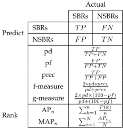
To evaluate the performance of the prediction models built with FARSEC filtered data, as well as the ranked bug reports, we use the measures shown in Figure 3. For the per-formance of the prediction models, the confusion matrix in Figure 3 is used, where TP, TN, FP and FN are true positive, true negative, false positive and false negative respectively. We report the probability of detectionpd, probability of false alarmpf, precision, f-measures and g-measures. Probability of detection measures the fraction of the actual SBRs the predictor finds The probability of false alarm measures the fraction of the NSBRs that are incorrectly predicted as SBRs. Precision (prec) measures the fraction of actual SBRs in the predicted SBRs. Actual SBRs NSBRs Predict SBRs T P F N NSBRs F P T N pd T P T P+F N pf F PF P+T N prec T P T P+F P
f-measure 2pd∗pd+∗precprec g-measure 2×pdpd+(100×(100−−pfpf)) Rank APn Pn k=1 P(k) n MAPn P N i=1 APni N
Fig. 3. Confusion matrix: Definitions of pd, pf, prec, g-measure and the mean average precision (MAP).
Thef-measureandg-measureare calculated using the pd, prec and pf values. The f-measure is the harmonic mean between pd and prec. The optimal f-measure value is 100%. The g-measure is the harmonic mean of pd and (100-pf).
100-pfrepresents a value is known asspecificity(not predict-ing NSBRs as SBRs). Specificity is used together with pd to form the G-mean2measure, which is the geometric mean of
the pds for both the majority and the minority classes [47]. In our case, we use these to form the g-measure. Finally, to measure any significant differences between the non-filtered and FARSEC non-filtered results, we use a two-tailed Mann Whitney statistical test with 95% confidence [48].
To determine the usefulness of FARSEC for ranked lists of bug reports, we use mean average precision (MAP) [49]. MAP is a metric used in information retrieval to measure the relevance of the topn results of a query. We use MAP to show that FARSEC ranking can return results with actual SBRs closer to the top of the list of all predicted SBRs. The formulas to calculate MAP are shown in the last row of Figure 3, where theaverage precision (AP)and then MAP are calculated. The average precision is measured cumulatively up to n which is the number of predicted SBRs, P(k) is the precision at point k in the list of bug reports. For our experiments, we divided the test data into deciles and the M APnis calculated cumulatively for each decile.
5
E
XPERIMENTD
ESIGN ANDR
ESULTSTo evaluate FARSEC, we use both the within and transfer learning techniques for building prediction models (recall Section 2.2.2). We denote these as Within Project Prediction (WPP) and Transfer Project Prediction (TPP) respectively. In our context, WPP uses labelled, historical bug reports from a project to predict SBRs in the unlabelled bug reports of the same project. TPP uses labelled bug reports from one project (but could be from many projects), to predict unlabelled bug reports of another project. We refer to the labelled data from other projects as thesource and the unlabelled data for the project we are building the predictor for, as thetarget.
In this paper we build WPP and TPP models using datasets that are unfiltered, FARSEC filtered, and CLNI filtered. WPP can be used when a project has enough historical data to build prediction models. TPP is used for projects with insufficient data available to build prediction models. When preparing data for TPP, we use security related keywords from the source to construct the term-document frequency matrix and the predictor for the target project.
Table 2 shows the outcome of applying different filters in terms of the number of remaining bug reports and the SBR %. Since we only remove NSBRs with a score above 0.75, the number of SBRs remain the same with and without filtering. This allows for an increase in the percentage of SBRs for building prediction models. There are four interest-ing cases shown in the table. The first two are thefarsecsq andclnifarsecsqfilters for Derby. The prediction models are built with training data where the majority are SBRs, 81% and 96% respectively. The last two cases concern the limited reduction withfarsectwoandfarsecfor Chromium. This is due to the threshold used to distinguish between NSBRs and SBRs. There are few Chromium reports with scores≥0.75.
All experiments are designed around the research ques-tions posed in the Section 1.
• RQ1: Can security cross words lead to mislabelled security bug reports by prediction models?
• RQ2: How do we buildeffectiveprediction models for security bug reports when data scarcity is an issue?
TABLE 2
Characteristics of the training data
Source Filter #SBRs #BRs SBRs(%) Chromium train 77 20970 0.4 farsecsq 14219 0.5 farsectwo 20968 0.4 farsec 20969 0.4 clni 20154 0.4 clnifarsecsq 13705 0.6 clnifarsectwo 20152 0.4 clnifarsec 20153 0.4 Wicket train 4 500 0.8 farsecsq 136 2.9 farsectwo 143 2.8 farsec 302 1.3 clni 392 1.0 clnifarsecsq 46 8.7 clnifarsectwo 49 8.2 clnifarsec 196 2.0 Ambari train 22 500 4.4 farsecsq 149 14.8 farsectwo 260 8.5 farsec 462 4.8 clni 409 5.4 clnifarsecsq 76 28.9 clnifarsectwo 181 12.2 clnifarsec 376 5.9 Camel train 14 500 2.8 farsecsq 116 12.1 farsectwo 203 6.9 farsec 470 3.0 clni 440 3.2 clnifarsecsq 71 19.7 clnifarsectwo 151 9.3 clnifarsec 410 3.4 Derby train 46 500 9.2 farsecsq 57 80.7 farsectwo 185 24.9 farsec 489 9.4 clni 446 10.3 clnifarsecsq 48 95.8 clnifarsectwo 168 27.4 clnifarsec 435 10.6
• RQ3: How do we generateusefullists of ranked bug
reports?
To answer the research questions we first generate datasets for our experiments by organizing the bug reports into training and test data (see Section 4.1). We then apply the text mining steps described in Section 3.1. Recall that some suspected SBRs have been publicly disclosed due to the lack of security domain knowledge of some bug re-porters [3] and also by those with knowledge who disregard requests to submit these reports privately [4]. Therefore, for our experiments we use past data to predict the present. The present represents any new unlabelled or mislabelled bug reports entering the bug tracking system. Once in the system, they are available publicly, therefore to avoid any suspected SBRs being made public before they are accessed, it is important to identify them and direct them to the security engineers.
Table 3 shows the total number of experiments per-formed. With five machine learning algorithms, eight treat-ments and four sources for WPP and TPP, we perform a
TABLE 3
Number of prediction models for each dataset
Treatments Prediction Models Total
WPP 1 data set×
5 machine learning algorithms×
8 (train + FARSEC filtering + CLNI) 40
TPP 1 data set×
4 sources×
5 machine learning algorithms×
8 (train + FARSEC filtering + CLNI) 160
Total 200
total of 200 experiments on each project. The following section describes the approach and results which answer each research question.
5.1 RQ1: Can security cross words lead to mislabelled security bug reports by prediction models?
Approach.To determine whether security cross words can cause bug reports to be mislabelled by prediction models, we compare FARSEC filters with the CLNI filter. While FAR-SEC filters are designed to reduce the number of security cross words in prediction models, the CLNI filter removes noisy NSBRs. We do two comparisons between the two filter types. The first is in terms of the reduction of the number of security cross words in the training data after filtering. The second is in terms of the number of SBRs mislabelled by the prediction models, which are created with the filtered data. To determine the number of security cross words in training data, we first need to generate the feature sets for each project (Section 3.1). From the feature sets, we use tf-idf as an indicator for security cross words. Any keyword with a tf-idf value above zero is considered to be a security cross word, i.e. present in both SBRs and NSBRs. The number of mislabelled SBRs are found by building WPP models with the filtered training data and machine learning algorithms (described in Section 4.3). The models are then evaluated with the test data.
Results. FARSEC filters reduce the number of security cross words in training data leading to fewer mislabelled SBRs by WPP models.Table 4 shows the number of security cross words present in the NSBRs of the training data before and after filtering. It also shows the top 100 security related keywords, sorted in descending order of their tf-idf values, for each project (feature sets) used in this paper. Highlighted are the keywords that are not security cross words before filtering. Notably, while the number of security cross words in Chromium has minor reductions with FARSEC filters, the other projects have reductions to as low as one word for Derby (the word is create). Overall, the median percentage decrease of security cross words for the CLNI filter is 0.4% while for FARSEC filters it is 39%.
When viewing these reductions in conjunction with WPP results in Table 5, we see that in most cases, the FARSEC filters reduces the number of mislabelled SBRs (shown in the FN column). In most cases, the CLNI filter either main-tains or increases the number of mislabelled SBRs when compared with the non-filtered results (train). The exception is Camel where the CLNI reduced the mislabelled reports from16to15.
TABLE 4
Top 100 security related keywords with the number of security cross words (the highlighted keywords are not security cross words)
Source Security Cross Words (SCWs) Security Related Keywords Filter # SCWs Chromium train farsecsq farsectwo farsec clni clnifarsecsq clnifarsectwo clnifarsec 100 95 100 100 100 95 100 100
file security chrome page http download user starred person notified changes may see url site bug open google browser like windows window https web code one memory firefox function tests problem seems tab also version use would using view used make users chromium crash click password think vulnerability sure browsers link attached attacker data get fix const content something safari new error javascript lcamtuf malicious please could risk release try found allow expected time example corruption test back access crashes urls int without know versions way uses cause fail want system still files arbitrary html details ssl need loaded might
Wicket train farsecsq farsectwo farsec clni clnifarsecsq clnifarsectwo clnifarsec 74 12 13 40 74 12 13 40
statelesshomepageattached callsdataproviderregards component limited files countjancouple database integer entries reason page get first java error unknown source signinform jetty requestlistenerinterfacecredentialsexpectedparams http exception interfacerequest homepage manually become inform stateful listener happends statelesschecker insucceeded creates causessucessfull opensactualfinalabstractlistenerquickstart mvn loginanalysisopenunpack
temporary enter signvaluemaphappystatelessproblemsigninpanel requestcycle occured fix delete deleting fails upload org webapplication hole space created handle example secu-rity server find important method multipart easy hope makes incomplete cancelled think workaround uploadingparserequestwant really anyonedisklargeeatingbug throwposting
developers call threadsservletwrapper
Ambari train farsecsq farsectwo farsec clni clnifarsecsq clnifarsectwo clnifarsec 95 25 57 88 94 25 57 88
security wizard service secure fails permissions allow start validation user cluster cannot set make page configs datanode add use default property name request instead enable web ssl password used services error disable fix permission options executed setup http nagios registration hosts also change url configuration try enabling check disabled host install time return provide call script issue file failures principaltouchedincorrect artifactsassignments
slaves side username directory path customizedeffectsmode unwanted false causes broken primary testmode mapred names working httpd state missingnavigation ganglia prepare
locked master ambari smoke wrong hbase node test zookeeper back need either true Camel train farsecsq farsectwo farsec clni clnifarsecsq clnifarsectwo clnifarsec 88 27 47 82 88 27 47 82
message http endpoint header org would uri component files also issue stop expose see static jetty endpoints specified port processing login route file error one messages headers support server lines using throws provide currently instance ftp sent means use issues ignore license dslinterfacesopened host fails redeliveryauthinterceptsendtoendpoint used connection check
memory heapnabblehttp bundles consumer pass path new case based classes however default-errorhandlerpushing expectedbody resultendpointexchange following exception else apache nullinoptionalouthandler token custom ignores servers something like protectedsftpendpoint
remove jms concatenateddelegateunderlyingsshdata copyftpcomponentmethod second csv results mockendpoint false
Derby train farsecsq farsectwo farsec clni clnifarsecsq clnifarsectwo clnifarsec 95 1 72 90 94 1 70 89
org security server test derbypermissionjava using access tests error support denied junit file exception database code user read manager locale run fails need version fail running
securitymanager network following files call required statement source table connect class thread blocksecurityexceptionwould used like failed problemprivilegedclient see jdbc set methodfilepermission trying granted authentication needs directory connection new think encryption sun jar policy start stack unknown rows revoke found information alpha thrown without name one create end update http could make trigger though native contains looks two key mode results sql use int classpath message incorrectly check
Taking a closer look at the results in Table 5, the farsec filter has a relatively similar performance to CLNI. For three out of five projects, their numbers of mislabelled SBRs match. This could be due to the fact that the filter does not use a bias on the keywords found in the SBRs (Section 3.2). However for Wicket and Derby, the farsec filter produces fewer mislabelled SBRs than the CLNI filter. This could be due to the average percentage decrease of security cross words for thefarsecfilter, which is 32 times larger than that of CLNI.
There are other notable results that can be gleaned from Table 5. First, there is no significant difference in the f-measure and g-f-measure results for each filter over the five projects. We used a two-tailed Mann Whitney test at 95% confidence. The results of the statistical test are not robust when the population size is less than 10. Therefore, we are cautious about conclusions formed based on this. Second, there does not seem to be any preference for a machine learning algorithm. Although each project has one dominant algorithm preference, others also contribute. An interesting
case is ib_k which only appears for Derby and only in the cases where the SBRs are the majority in the training data, i.e. with filters farsecsq and clnifarsecsq (Table 2). Finally, the bold results in the table show that the FARSEC filters (clnifarsecsq and farsectwo) overall, had relatively better performance than the other filters according to the g-measures.
5.2 RQ2: How do we buildeffectiveprediction models for security bug reports when data scarcity is an issue? Approach.When data scarcity is an issue, transfer learning is used to build prediction models (Section 2.2.2). We define an effective TPP model as one whose performance is com-parable to or better than that of WPP models. Therefore, to build effective TPP models for SBRs, we use the training data from the previous experiment for WPP models as the source and generate new test data based on their feature sets. For example, if the Wicket project is new and has little or no data to build a prediction model, we can use Ambari or another project as the source. Therefore the feature set
TABLE 5
WPP results with FARSEC and CLNI filtering (those with the highest g-measures are highlighted)
Target Filter Learner TN TP FN FP pd pf prec f-measure g-measure
Chromium train logistic regression 20815 18 97 40 15.7 0.2 31.0 20.8 27.1
farsecsq random forest 20801 17 98 54 14.8 0.3 23.9 18.3 25.7
farsectwo logistic regression 20815 18 97 40 15.7 0.2 31.0 20.8 27.1
farsec logistic regression 20815 18 97 40 15.7 0.2 31.0 20.8 27.1
clni logistic regression 20808 18 97 47 15.7 0.2 27.7 20.0 27.1
clnifarsecsq multilayer perceptron 20066 57 58 789 49.6 3.8 6.7 11.9 65.4
clnifarsectwo logistic regression 20808 18 97 47 15.7 0.2 27.7 20.0 27.1
clnifarsec logistic regression 20808 18 97 47 15.7 0.2 27.7 20.0 27.1
Wicket train naive bayes 459 1 5 35 16.7 7.1 2.8 4.8 28.3
farsecsq logistic regression 305 4 2 189 66.7 38.3 2.1 4.0 64.1
farsectwo logistic regression 313 4 2 181 66.7 36.6 2.2 4.2 65.0
farsec logistic regression 454 2 4 40 33.3 8.1 4.8 8.3 48.9
clni naive bayes 467 0 6 27 0.0 5.5 0.0 0.0 0.0
clnifarsecsq logistic regression 368 2 4 126 33.3 25.5 1.6 3.0 46.1
clnifarsectwo logistic regression 357 2 4 137 33.3 27.7 1.4 2.8 45.6
clnifarsec logistic regression 442 3 3 52 50.0 10.5 5.5 9.8 64.2
Ambari train multilayer perceptron 485 1 6 8 14.3 1.6 11.1 12.5 24.9
farsecsq random forest 422 3 4 71 42.9 14.4 4.1 7.4 57.1
farsectwo random forest 478 4 3 15 57.1 3.0 21.1 30.8 71.9
farsec multilayer perceptron 469 1 6 24 14.3 4.9 4.0 6.3 24.8
clni multilayer perceptron 480 1 6 13 14.3 2.6 7.1 9.5 24.9
clnifarsecsq random forest 455 4 3 38 57.1 7.7 9.5 16.3 70.6
clnifarsectwo random forest 471 2 5 22 28.6 4.5 8.3 12.9 44.0
clnifarsec random forest 493 1 6 0 14.3 0.0 100.0 25.0 25.0
Camel train logistic regression 464 2 16 17 11.1 3.5 10.5 10.8 19.9
farsecsq random forest 426 3 15 55 16.7 11.4 5.2 7.9 28.1
farsectwo logistic regression 280 9 9 201 50.0 41.8 4.3 7.9 53.8
farsec logistic regression 448 3 15 33 16.7 6.9 8.3 11.1 28.3
clni naive bayes 422 3 15 59 16.7 12.3 4.8 7.5 28.0
clnifarsecsq multilayer perceptron 415 3 15 67 16.7 13.9 4.3 6.8 27.9
clnifarsectwo multilayer perceptron 445 2 16 37 11.1 7.7 5.1 7.0 19.8
clnifarsec logistic regression 458 3 15 24 16.7 5.0 11.1 13.3 28.4
Derby train naive bayes 427 16 26 31 38.1 6.8 34.0 36.0 54.1
farsecsq ib k 321 23 19 137 54.8 29.9 14.4 22.8 61.5
farsectwo random forest 401 20 22 57 47.6 12.4 26.0 33.6 61.7
farsec naive bayes 429 16 26 29 38.1 6.3 35.6 36.8 54.2
clni random forest 456 10 32 2 23.8 0.4 83.3 37.0 38.4
clnifarsecsq ib k 321 23 19 137 54.8 29.9 14.4 22.8 61.5
clnifarsectwo random forest 416 15 27 42 35.7 9.2 26.3 30.3 51.3
clnifarsec naive bayes 427 16 26 31 38.1 6.8 34.0 36.0 54.1
of Ambari is used by Wicket to calculate the frequencies of each keyword for each bug report. In the end we have a test set for Wicket based on the feature set of another project. Note that in the context of our experiments, scarcity can also mean little or no SBRs present for building the models. As shown in Table 3, we build 160 TPP models in our ex-periments, including the use of filtered sources. To evaluate the effectiveness of these models, we compare them with the WPP models. Specifically, we determine if the performance of the TPP models has degraded or improved from the WPP models in terms of f-measure, g-measure and the number of mislabelled SBRs. We use the Mann Whitney statistical test for comparison.
Results. When data scarcity is an issue, other sources can be used to build effective prediction models. Table 6 shows the best TPP results with FARSEC and CLNI filtering (according to f-measures). From these results, theboldones indicate those with the highest g-measures.
Overall, there is no significant difference in TPP model performances when compared with WPP models. This is the case for the f-measures, g-measures and the number of mislabelled SBRs. However, a closer look at the results in Table 6 reveals five notable points:
1) TPP models for train and CLNI improve the f-measures and g-f-measures for the projects with the lowest number of SBRs in their training data (i.e. Wicket, Ambari and Camel). This confirms the use-fulness of TPP when dealing with data scarcity, especially when SBRs are few. Furthermore, for Chromium and Derby, the CLNI filter TPP model has higher g-measures than its WPP counterparts. 2) The pfs for the TPP models are all below 25% while
some of the FARSEC filtering WPP models have pfs above 25%. Namely Wicket, Camel and Derby. 3) No single source stands out. FARSEC filtered
Chromium is the best source for Ambari and Derby. Ambari works best for Chromium, Derby is best for Camel and Camel is best for Wicket. However Wicket only works well for Derby, but it is not the best result.
4) Similar to the WPP result, there is no preference for a particular machine learning algorithm. However, except for Wicket, each project has a dominant al-gorithm. For Chromium it israndom_forestand for Ambari it ismultilayer_perceptron. Camel and Derby work best with naive_bayes. Unlike the WPP results,ib_k, does not appear for any of
TABLE 6
TPP results with FARSEC and CLNI filtering (those with the highest g-measures are highlighted)
Target Source Filter Learner TN TP FN FP pd pf prec f-measure g-measure
Chromium Derby train random forest 20835 2 113 20 1.7 0.1 9.1 2.9 3.4
Ambari farsecsq random forest 19279 34 81 1576 29.6 7.6 2.1 3.9 44.8
Ambari farsectwo random forest 20454 53 62 401 46.1 1.9 11.7 18.6 62.7
Derby farsec multilayer perceptron 20502 12 103 353 10.4 1.7 3.3 5.0 18.9
Camel clni logistic regression 20262 25 90 593 21.7 2.8 4.0 6.8 35.5
Ambari clnifarsecsq random forest 19817 56 59 1038 48.7 5.0 5.1 9.3 64.4
Derby clnifarsectwo random forest 20332 26 89 523 22.6 2.5 4.7 7.8 36.7
Camel clnifarsec multilayer perceptron 20590 8 107 265 7.0 1.3 2.9 4.1 13.0
Wicket Camel train naive bayes 437 3 3 57 50.0 11.5 5.0 9.1 63.9
Chromium farsecsq multilayer perceptron 475 1 5 19 16.7 3.8 5.0 7.7 28.4
Camel farsectwo random forest 490 1 5 4 16.7 0.8 20.0 18.2 28.5
Camel farsec naive bayes 431 3 3 63 50.0 12.8 4.5 8.3 63.6
Ambari clni multilayer perceptron 476 1 5 18 16.7 3.6 5.3 8.0 28.4
Chromium clnifarsecsq random forest 493 1 5 1 16.7 0.2 50.0 25.0 28.6
Camel clnifarsectwo random forest 489 1 5 5 16.7 1.0 16.7 16.7 28.5
Camel clnifarsec naive bayes 433 3 3 61 50.0 12.3 4.7 8.6 63.7
Ambari Derby train multilayer perceptron 484 2 5 9 28.6 1.8 18.2 22.2 44.3
Chromium farsecsq multilayer perceptron 474 3 4 19 42.9 3.9 13.6 20.7 59.3
Chromium farsectwo naive bayes 472 3 4 21 42.9 4.3 12.5 19.4 59.2
Camel farsec multilayer perceptron 492 1 6 1 14.3 0.2 50.0 22.2 25.0
Derby clni multilayer perceptron 477 2 5 16 28.6 3.2 11.1 16.0 44.1
Chromium clnifarsecsq random forest 492 1 6 1 14.3 0.2 50.0 22.2 25.0
Chromium clnifarsectwo naive bayes 474 2 5 19 28.6 3.9 9.5 14.3 44.1
Camel clnifarsec multilayer perceptron 492 1 6 1 14.3 0.2 50.0 22.2 25.0
Camel Derby train naive bayes 457 3 15 24 16.7 5.0 11.1 13.3 28.4
Chromium farsecsq naive bayes 401 7 11 80 38.9 16.6 8.0 13.3 53.0
Derby farsectwo naive bayes 371 8 10 110 44.4 22.9 6.8 11.8 56.4
Ambari farsec logistic regression 439 5 13 42 27.8 8.7 10.6 15.4 42.6
Ambari clni logistic regression 444 5 13 37 27.8 7.7 11.9 16.7 42.7
Chromium clnifarsecsq naive bayes 402 7 11 79 38.9 16.4 8.1 13.5 53.1
Ambari clnifarsectwo random forest 455 3 15 26 16.7 5.4 10.3 12.8 28.3
Derby clnifarsec multilayer perceptron 473 2 16 8 11.1 1.7 20.0 14.3 20.0
Derby Ambari train naive bayes 393 13 29 65 31.0 14.2 16.7 21.7 45.5
Chromium farsecsq naive bayes 370 19 23 88 45.2 19.2 17.8 25.5 58.0
Ambari farsectwo random forest 454 6 36 4 14.3 0.9 60.0 23.1 25.0
Wicket farsec naive bayes 354 19 23 104 45.2 22.7 15.4 23.0 57.1
Ambari clni naive bayes 400 12 30 58 28.6 12.7 17.1 21.4 43.1
Chromium clnifarsecsq naive bayes 372 19 23 86 45.2 18.8 18.1 25.9 58.1
Ambari clnifarsectwo random forest 449 8 34 9 19.0 2.0 47.1 27.1 31.9
Wicket clnifarsec naive bayes 363 18 24 95 42.9 20.7 15.9 23.2 55.6
the projects.
5) Apart from Wicket, the FARSEC filtered models worked best for all the projects (according to their g-measures shown in Table 6). In addition, these best results had lower numbers of mislabelled SBRs than the train and CLNI models. For Wicket, the farsec and clnifarsec filters are comparable to the best result (train) with matching number of predicted SBRs (TPs).
5.3 RQ3: How do we generate useful lists of ranked bug reports?
Approach.Results in Table 5 and Table 6, show that some of the best results with FARSEC filtering have high FPs, while results without filtering tend to have lower FPs. For a security engineer, using an approach with high FPs is akin to “finding a needle in a haystack” [5], and is not useful even if there are more SBRs in the results. In order to alleviate this problem we generate useful lists of ranked bug reports, sorted according to the steps described in Section 3.3. For non-filtered WPP and TPP models we rank the bug reports using Step 1 and Step 2 described in Section 3.3. For the models built with FARSEC filtered data, we follow both
steps in Section 3.3. This sorts the prediction results with the least number of predicted SBRs with those from the FARSEC filters. This ranking method takes advantage of the lower FPs even if there is only one actual SBR present. We evaluate it using the cumulative mean average precision (MAP) over 10 deciles (see Figure 3).
Results. SBRs are ranked relatively highly with FAR-SEC.The cumulative MAPs over deciles of the best predic-tion results for each project are shown in Table 7. The left column shows the results for WPP and the right column, TPP. Each chart has abaseline, train (non-filtered results) and CLNI results. The baseline is the bug reports ranked chrono-logically (i.e., ascending order of the bug report numbers). For clarity, we have generated four charts for each project to show any differences in results for FARSEC filters with and without CLNI. The ranked lists with the higher MAP values show that more actual SBRs are closer to the top of the lists. Overall, FARSEC ranking shows promise, outperform-ingtrainandCLNI results in nine out of ten cases Table 7. The exception is the CLNI results for Derby shown in the chartsqand r, where CLNI at the first decile outperforms train and the FARSEC filters. However from the second decile onward,farsectwohas the highest MAP.
TABLE 7
The cumulative MAPs over deciles of the best prediction results for each project.
WPP TPP
(a) Chromium MAP (b) Chromium MAP (c) Chromium MAP (d) Chromium MAP
(e) Wicket MAP (f) Wicket MAP (g) Wicket MAP (h) Wicket MAP
(i) Ambari MAP (j) Ambari MAP (k) Ambari MAP (l) Ambari MAP
(m) Camel MAP (n) Camel MAP (o) Camel MAP (p) Camel MAP
(q) Derby MAP (r) Derby MAP (s) Derby MAP (t) Derby MAP
1) The CLNI ranking for Wicket performs worse than the baseline. This agrees with the results in Table 5, which shows zero predicted actual SBRs.
2) For Chromium and Derby, their TPP rankings are relatively worse than WPP. For Wicket, Ambari and Camel, the opposite is true. Their TPP ranking for train, CLNI and the FARSEC filters were relatively better than their WPP rankings.
3) For a few cases where the best results in Table 5 and Table 6 show high FPs, we found that they did
not produce the best ranked results in Table 7. In-stead they were generally inferior to other FARSEC ranked results. For instance, Table 5 showed Wicket to achieve the best result withfarsectwo, however, bothfarsecandclnifarsechad better rankings. An-other example in WPP is Camel, wherefarsectwois out-ranked by the other FARSEC ranked results. For the best TPP results with high FPs, Chromium and Camel are out-ranked by farsectwo and farsecsq respectively. This shows that FARSEC ranking can