UC San Diego
UC San Diego Electronic Theses and Dissertations
Title
Learning Application-Oriented Classifiers for Multi-frame Visual Recognition Permalink https://escholarship.org/uc/item/7t6276x7 Author Pal, Anwesan Publication Date 2019 Peer reviewed|Thesis/dissertation
UNIVERSITY OF CALIFORNIA SAN DIEGO
Learning Application-Oriented Classifiers for Multi-frame Visual Recognition
A thesis submitted in partial satisfaction of the requirements for the degree
Master of Science
in
Electrical and Computer Engineering
by
Anwesan Pal
Committee in charge:
Professor Henrik I Christensen, Chair Professor Nuno Vasconcelos, Co-Chair Professor Nikolay Atanasov
Copyright Anwesan Pal, 2019
The thesis of Anwesan Pal is approved, and it is acceptable in quality and form for publication on microfilm and electroni-cally:
Co-Chair
Chair
University of California San Diego
DEDICATION
TABLE OF CONTENTS
Signature Page . . . iii
Dedication . . . iv
Table of Contents . . . v
List of Figures . . . vii
List of Tables . . . ix
Acknowledgements . . . x
Vita . . . xi
Abstract of the Thesis . . . xii
Chapter 1 Introduction . . . 1
1.1 Bias in Action Recognition . . . 2
1.2 Visual Place Categorization . . . 4
1.3 Attention in Action Recognition . . . 6
1.4 Overview of the Thesis . . . 6
Chapter 2 Representation Bias in Datasets and Algorithms . . . 8
2.1 Background . . . 8 2.2 Understanding a Dataset . . . 10 2.2.1 Bias . . . 10 2.2.2 Fairness . . . 11 2.2.3 Representations . . . 11 2.2.4 Algorithms . . . 14 2.3 Experiments . . . 15 2.3.1 Representation bias . . . 15
2.3.2 Effect of bias on algorithms . . . 20
2.3.3 Effect of Dataset Manipulation on Algorithms . . . 22
2.4 Conclusion . . . 24
Chapter 3 Diverse Scene Detection . . . 25
3.1 Background . . . 25
3.2 Proposed Methodology . . . 27
3.2.1 Scene Recognition . . . 28
3.2.2 Object Detection . . . 28
3.2.3 Place Categorization models . . . 28
3.3.1 Training Procedure . . . 31
3.3.2 Experiment Settings . . . 32
3.4 Conclusion . . . 37
Chapter 4 Visual Attention Mechanism for Action Classification . . . 40
4.1 Background . . . 40
4.2 Proposed Methodology . . . 41
4.2.1 Camera motion estimation and scene structure in video frames 41 4.2.2 Neural Networks . . . 44
4.3 Technical Approach . . . 47
4.3.1 Data Collection and Pre-processing . . . 47
4.3.2 Model Architecture and hyper-parameters . . . 49
4.4 Results and Discussion . . . 49
Chapter 5 Conclusion and Future Work . . . 53
LIST OF FIGURES
Figure 1.1: Extreme classes for different Representation Biases . . . 3
Figure 1.2: Visualization of the semantic mapping performed while the Fetch robot is navigating through the environment. . . 5
Figure 2.1: Dominant representation bias . . . 16
Figure 2.2: Characterization of bias skew of all datasets for saliency . . . 17
Figure 2.3: Box-plots of the strength of largest bias (”a”) and the rate of bias decay (”b”) for different datasets . . . 18
Figure 2.4: Correlation coefficients for average class bias and fairness score versus class frequency . . . 19
Figure 2.5: PCA visualization of the algorithms and representations projected onto the space of the two largest Principal Components . . . 21
Figure 2.6: t-SNE visualization of clusters of UCF101 classes and the corresponding algorithm performance on each cluster . . . 22
Figure 2.7: Performance of two algorithms on UCF101 and their differences, with biased classes removed. . . 23
Figure 3.1: Model Architecture. The highlighted regions represent the portion of the network which was trained for the respective models. . . 27
Figure 3.2: Architecture for Generation of the Activation Map. The 14x14 feature maps obtained from the block layer 4 of WideResNet are combined with the weights from the final FC layer, and then their dot product id upsampled to the image size and overlaid on top to get the activation maps . . . 30
Figure 3.3: Detection Results on Real-World Videos. Top row corresponds to the video of a Real-Estate model house. The next 2 rows are from the houses of the authors and their friends. The bottom row is obtained from a house in the movie”Father of the Bride”. . . 35
Figure 3.4: Place categorization experiments with mobile robots. Each color represents one of the seven classes of the visual place categorization that our system classified. . . 39
Figure 4.1: From left to right: Comparison of early-fusion, late-fusion, and two-stream methods. . . 41
Figure 4.2: Diagram of computing optical Flow via Lucas-Kanade Method. In the above image, optical flow gives the velocity gradients of the pixels which move in position over time. In the lower image, we highlight the portion of the image which is in motion (the vehicles). . . 43
Figure 4.3: Neural network architectures used . . . 44
Figure 4.4: The structure of the Convolutional network encoder. . . 45
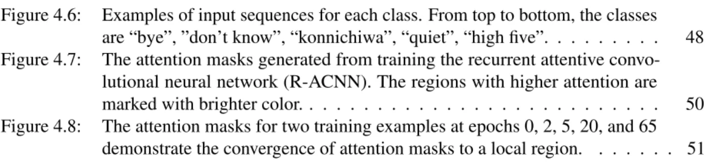
Figure 4.6: Examples of input sequences for each class. From top to bottom, the classes are “bye”, ”don’t know”, “konnichiwa”, “quiet”, “high five”. . . 48 Figure 4.7: The attention masks generated from training the recurrent attentive
convo-lutional neural network (R-ACNN). The regions with higher attention are marked with brighter color. . . 50 Figure 4.8: The attention masks for two training examples at epochs 0, 2, 5, 20, and 65
LIST OF TABLES
Table 2.1: Representation bias of the various datasets. . . 13
Table 3.1: Top landmark objects (non-human) for the seven different scene classes . . 29
Table 3.2: Accuracy in percentage of DEDUCE on Places365 dataset . . . 32
Table 3.3: Accuracy in percentage of DEDUCE on SUN dataset . . . 33
Table 3.4: VPC Dataset: Average Accuracy across the 6 home environments . . . 34
Table 3.5: VPC Dataset: Comparison with State Of The Art . . . 34
ACKNOWLEDGEMENTS
I wish to extend my sincerest gratitude to my advisor, Dr. Henrik I Christensen for his help and guidance towards the work contained in this thesis. I have learnt a tremendous amount through the discussions that we have had together. This thesis would not have been what it is without him.
I am very grateful to the rest of the members of my committee namely, Dr. Nuno Vasconcelos and Dr. Nikolay Atanasov for their invaluable insights and constructive criticisms. I am also indebted to my fellow graduate students, Ahmed H. Qureshi, Carlos Nieto-Granda, Zhihang Ren, Yi Li, Shixin Li, James Smith and Priyam Parashar for their helpful comments and support.
I am eternally grateful to my parents, my elder brother and his wife for their constant motivation and unwavering faith in me. Their love and encouragement has been critical for the successful completion of my degree.
This thesis is currently being prepared for submission for publication of the material. Pal, Anwesan - The thesis author was the primary investigator and author of this material.
VITA
2017 Bachelor of Engineering, Indian Institute of Engineering Science and Technology, Shibpur
2017-2018 Teaching Assistant, University of California San Diego
2018-Present Research Assistant, University of California San Diego 2019 (Expected) Master of Science, University of California San Diego
PUBLICATIONS
Anwesan Pal, Carlos-Nieto Granda and Henrik I Christensen “DEDUCE: Diverse scEne De-tection methods in Unseen Challenging Environments”, submitted to IEEE/RSJ International Conference on Intelligent Robots and Systems (IROS), 2019.
Anwesan Pal, Zhihang Ren, Yi Li, Nuno Vasconcelos and Henrik I Christensen “A Deeper Look at Action Recognition Datasets and Algorithms via Representation Bias”, submitted to IEEE Conference on Computer Vision and Pattern Recognition (CVPR), 2019.
Xinran Li∗,Anwesan Pal∗, Ahmed Qureshi and Carlos-Nieto Granda “Optical Flow Based Video Classification with Visual Attention using Recurrent Convolutional Neural Network”,presented for a course project, 2018.
ABSTRACT OF THE THESIS
Learning Application-Oriented Classifiers for Multi-frame Visual Recognition
by
Anwesan Pal
Master of Science in Electrical and Computer Engineering
University of California San Diego, 2019
Professor Henrik I Christensen, Chair Professor Nuno Vasconcelos, Co-Chair
Classification, asupervised learningproblem, is a technique to categorize a given set of data points into two (binary classification) or more (multi-class classification) targets or labels, based on their characteristics. It has wide applications in the domain of Computer Vision and Robotics. Despite the tremendous success of classification in recent times, a fundamental question remains as to whether a classifier truly learns the correct representation (i.e. theground-truth representation) needed to solve a problem. The uncertainty in learning often limits generalization of such methods across different domains. This thesis presents an in-depth study of how different classifiers leverage the intrinsic properties of a dataset in order to robustly model the data
distribution. The study further extends to the application of classifiers in two challenging domains - Visual Semantic Place Categorization and Human Activity Recognition.
The first part of the thesis focuses on the concept of bias in action recognition videos. This is illustrated by the fact that given just a single frame of a video, some actions can be easily identified, due to the presence of certain objects and the background. The second part generalizes classification into the domain of place categorization, where the focus is to learn semantic information about a robot’s environment without any human guidance. This is done through a deep fusion of the scene and object attributes. Finally, an algorithm is proposed for human action recognition which incorporates the information learnt from optical flow and visual attention mechanism in order to perform classification.
Chapter 1
Introduction
Classification has always been an important topic in Machine Learning, and its appli-cations are now widely spreading into the domains of Computer Vision and Robotics. Images and videos are an excellent source of semantic information since they can capture detailed contextual cues in a setting which is not possible through other types of sensors like LiDAR, Proximity, Gyroscope etc. Deep Learning models invoking Convolutional Neural Networks (CNNs) [LBBH98] have been very successful in tackling problems related to images including recognition, segmentation and detection [KSH12, CGGS12, FCNL12, GDDM14]. However, videos, ormulti-frame recognitionbring in more challenges in itself, such as huge computational cost, need for capturing long context, network architectural design constraints and lack of standard evaluation benchmarks. This thesis talks about these challenges in detail, with a special emphasis on what intrinsic properties are learnt by a deep learning model in order to solve the classification problem. The applications are discussed in the context of semantic place categorization and human action classification.
1.1
Bias in Action Recognition
The introduction of deep learning has enabled substantial advances in computer vision over the last few years. This is mostly because deep learning networks [KSH12, SZ14, SLJ+15, HZRS16] can leverage large amounts of training data in order to learn sophisticated representa-tionsof images and videos that enable the robust solution of problems such as object or action recognition. On the other hand, these networks raise challenges because it is not very clear as to what exactly they learn. This makes it difficult to know how far beyond their training they can generalize. One well known principle in machine learning is that a learning system can only be as good as the data on which it is trained. If the dataset is not representative of the entire example distribution, the network will overfit. This is known as dataset bias [TE11] and can be combated by increasing dataset size. With modern datasets [RDS+15, KRA+18, LMB+14, KH09], which tend to be very large in size, and therefore dataset bias is less of an issue.
There are, nevertheless, other sources of bias. One particularly difficult example is
representation bias, i.e. the fact that the dataset favors some types of representations over others. Representation bias is unavoidable in recognition problems since the goal is to learn the optimal representation for the solution of the recognition problem, a.k.a. theground-truth representation. While it is usually unknown, some properties of this representation can be inferred from the definition of the recognition problem. For example, it is unlikely that a system for the classification of horse breeds will need to learn a representation of humans [DT05], as opposed to that of motion. This is because running style of different horses can be informative of its breed. This, however, assumes an ideal dataset. In practice, the dataset may be such that certain horse breeds always appear with humans (e.g. domestic horses) while others do not (e.g. wild horses).
When this happens, a representation of humans, such as a person detector [TAS14], will achieve better than chance level performance for horse classification. In this case, the dataset is said to bebiasedfor the human representation. In the extreme case, this might result in a very
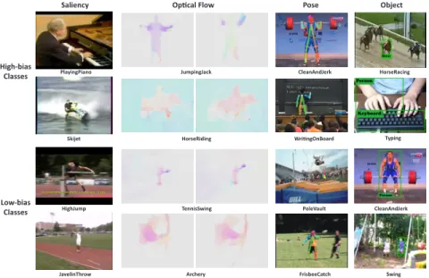
high recognition accuracy utilizing only human representations. It is likely here that the deep learning system has solved the problem without building any representation of horses. Unlike dataset bias, a difficulty of representation bias is that it is not necessarily eliminated by simply making datasets larger. In general, the problem is that the data collection is itself biased. For example, pictures commonly found on the web may pit domestic horses with humans while wild horses in seclusion. Thus, if additional data is acquired online, the representation bias will only be reinforced. Saliency PlayingPiano Skijet HighJump JavelinThrow High-bias Classes Low-bias Classes Op�cal Flow JumpingJack HorseRiding TennisSwing Archery CleanAndJerk Wri�ngOnBoard PoleVault FrisbeeCatch Pose Object HorseRacing Typing CleanAndJerk Swing
Figure 1.1: Representation bias illustrated by the frames of UCF101 classes. The features from these frames are given as inputs to the classifier. Top 2 rows correspond to the high-biased classes while the bottom 2 rows to the low-biased classes. Upon inspection, it is much simpler to classify the frames in the top rows into their respective classes as compared to the bottom rows.
In domains such as action recognition, representation bias is a complex problem because there are many potential sources of bias. Some of these are illustrated in Figure 1.1, with examples from the UCF101 [SZS12] dataset. For example, action classes such as ”playing piano” or ”jet ski” can be recognized by inspection of a single image, while ”jumping jack” and ”riding a horse” are easily recognized from short term motion patterns, ”Clean and Jerk” and ”Writing on board” from human pose skeleton, and finally classes such as ”horse racing” and ”typing” from the presence of certain objects. In summary, UCF101 has bias towards static, motion, pose, and
object representations.
Given all this, the characterization of representation bias of existing datasets is important for at least two reasons. First, it provides pointers on how to create or modify datasets so as reduce or eliminate bias. For example, Liet al. [LLV18] have recently proposed a measure of representation bias and used it to show that a dataset (Diving48) explicitly collected to have low bias, does not have to be particularly large [KCS+17, GKM+17, MBG+18]. Second, by analyzing the performance of different action recogniton algorithms on datasets with quantified biases, it is possible to infer properties of the representation learned by the algorithm. This enables a better understanding of where these algorithms are likely to succeed and fail and can be exploited to produce new algorithms that address these limitations. Given the flexibility of modern deep learning systems, they are quite likely to exploit any existing biases to learn representations that solve the dataset instead of the real action recognition problem.
1.2
Visual Place Categorization
Scene recognition and understanding has been an important area of research in the Robotics & Computer Vision community for more than a decade now. Programming robots to identify their surroundings is integral to building autonomous systems for aiding humans in house-hold environments.
Kostaveliset al. [KG15] provided a survey of previous work in semantic mapping using robots in the last decade. According to their study, scene annotation augments topological maps based on human input or visual information of the environment. Bormannet al. [BJL+16] pointed out that the most popular approaches in room segmentation involve segmenting floor plans based on spatial regions.
An essential aspect of any spatial region is the presence of specific objects in it. Some examples include a bed in a bedroom, a stove in a kitchen, a sofa in a living room, etc. Nikoet
al. [SBS+18] formulated the following three reasoning challenges that address the semantics and geometry of a scene and the objects therein, both separately and jointly: 1) Reasoning About Object and Scene Semantics, 2) Reasoning About Object and Scene Geometry, and 3) Joint Reasoning about Semantics and Geometry. The content in this thesis focuses on the first reasoning challenge and uses Convolutional Neural Networks (CNNs) as feature extractors for both scenes and objects. The goal is to design a system that allows a robot to identify the area where it is located using visual information in a manner similar to how a human being would.
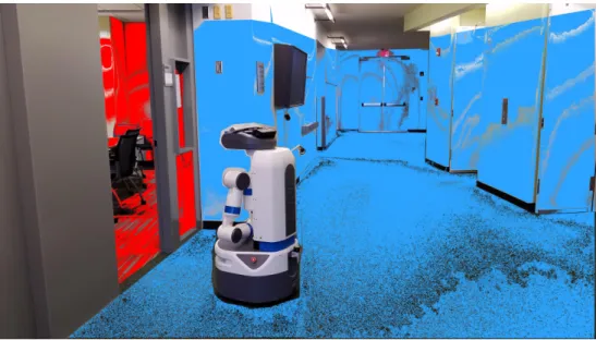
Figure 1.2: Visualization of the semantic mapping performed while the Fetch robot is navigating through the environment.
In this thesis, five different models of scene prediction have been considered, each developed through the integration of object and scene information from a surrounding in order to perform place categorization. To evaluate the robustness of these models, extensive experiments have been conducted on state-of-the-art still-image datasets, real-world videos captured via different hand-held cameras, and also those recorded using a mobile robot platform in multiple challenging environments. One such environment is shown in Figure 1.2, where the segmented regions correspond to the scenes detected. The results obtained from the experiments demonstrate that the proposed system can be generalized beyond the training data, in addition to being
impervious to object clutter, motion blur and varying light conditions.
1.3
Attention in Action Recognition
The study of attention has classically focused on the physical characteristics that determine whether stimuli are attended. William James [Jam50] defined attention as taking possession of one out of several simultaneously possible objects or train of thoughts by the mind. The modern study of attention continues to work within this broad definition. It is generally accepted that an individual is only aware of a small fraction of the information provided to the brain by the sensory systems.
The computer vision models of attention perform remarkably well in most of the applica-tions where static images or images from a video stream are manually fed to the model in order to identify the most salient/task-relevant stimuli. In case of some real-time applications where the current visual input of the attention model is to be determined by the decision output of the model (i.e., the focus of attention) at the immediate past, the traditional methods of visual attention face severe limitations in a number of aspects [BMG06], [BMGK08] and[BKMG09]. Using a visual attention model as a component of robotic cognition is an example of such applications. In this case, the attention model should be able to locate the behaviorally relevant stimuli in an ongoing stream of visual input and respond to it, perform learning in an on-line fashion and with minimal human supervision, and apply the learned knowledge for guiding the attention behavior in arbitrary environmental settings.
1.4
Overview of the Thesis
Chapter 2 presents a study of the representation biases of existing datasets through their results as reported. Six types of representation biases are defined and a procedure to quantify
them is proposed. For implementation, nine of the most popular action recognition datasets are considered. The characterization of bias is performed both at the level of the entire dataset and that of individual classes. This provides a detailed picture of the origin of the biases that can be leveraged by dataset creators to produce better datasets, either by adding data to the existing datasets or by assembling new ones. In addition, a set of prototypical deep learning algorithms for action recognition are also considered, and their performance are characterized in terms of bias. This provides some insight on the representations learned by the algorithms. Finally, it is shown that by simple manipulation of a small number of classes, it is possible to undermine the ”state of the art” standard for algorithm evaluation in computer vision.
Chapter 3 introduces a set of Diverse scEne Detection methods in Unseen Challenging Environments (DEDUCE) algorithms for performing visual semantic place categorization. These algorithms are then evaluated across different domains. The first experiments are conducted on two state of the art 2D image datasets. This is followed by more experiments on real world videos captured via professional and ordinary cell-phone cameras in house-hold settings. To further test the robustness of the algorithms, an experiment is also carried out on a recording of a movie, where the focus is not on the background, but instead on the people involved. Finally, data is recorded on a mobile robot navigating through an office setting and place categorization is performed without human guidance.
Chapter 4 provides a brief background of Optical Flow and the Neural Network architec-tures and algorithms implemented thus far for human action classification. This is followed by the explanation of the proposed Recurrent-Attentive Convolutional Neural Networks (R-ACNN) al-gorithm for video classification. Detailed description about the data collection and pre-processing, model architecture and hyper-parameter training are also provided. Finally, the results of the proposed algorithm is compared along with the other state of the art algorithms.
Chapter 2
Representation Bias in Datasets and
Algorithms
2.1
Background
The learning process for action recognition can be affected by a wide variety of biases. Many of these biases can be divided broadly into two categories based on the type of features they affect—static and dynamic. To mitigate static biases, early action recognition datasets, such as KTH [SLC04], Weizmann [BGS+05] and Hollywood2 [MLS09], were captured under a controlled environment. However, most classes of these datasets can be recognized by simply analyzing motion in small spatiotemporal neighborhoods. Also, these datasets are small and prone to overfitting. Recently, many datasets have appeared which are larger in size and contain more diverse classes, such as UCF101 [SZS12], HMDB51 [KJSS13] and Kinetics [KCS+17]. Unfortunately, these datasets do not cover a wide range of the daily life actions. To overcome this problem, Charades [SVW+16] and Something-Something (v1 and v2) [GKM+17, MBG+18] change the traditional way of labeling action classes and bring in more daily life videos. In Charades, most videos are about day-to-day actions and every single video is assigned multiple
motion labels. For the Something-Something datasets, class names are not associated with any object or identity, such as”Throwing something”,”Putting something on something”, etc. Another newly introduced dataset, Diving48 [LLV18], consists of videos of competitive diving, and has the added advantage of containing low static cues.
The notion that dataset bias can affect the performance of recognition systems has received some attention by the computer vision community. Torralbaet al.[TE11] uncovered biases of several image datasets and related them to the poor generalization performance of state-of-the-art models. Gkioxari et al.[GGM15] began to utilize contextual biases to solve action recognition. Tommasiet al.[TPCT17] performed a thorough analysis of the common datasets and verified the present de-biasing methods. More recently, Feichtenhoferet al.[FPWZ18] utilized network visualizations to understand dataset bias and Stocket al.[SC18] proposed a way to avoid undesirable bias when learning a model.
Traditional action recognition algorithms utilize different types of representations to boost their performance. In many cases, it is difficult to determine what biases these representations can leverage. There are, however, examples where the model uses a very explicit combination of elementary representations. For example, two stream networks [SZ14] implement spatial and temporal streams, which capture the static and dynamic structure of video respectively, and combine these results at the final layer. These models can leverage either static or dynamic biases to achieve artificially good performance on a biased dataset. The P-CNN of [CLS15] utilizes a ”guided” two stream network, which adds a pose representations to the mix. Because they are fairly explicit about their representations, these models are suitable tools for measuring the amount of bias of different datasets.
2.2
Understanding a Dataset
This section discusses the tools and the experiment setups used to measure bias. It also introduces the different biases considered and the algorithms tested.
2.2.1
Bias
Liet al.[LLV18] introduced the concept of representation bias, defining the amount of bias of a dataset
D
with respect to a representationφasB
(D
,φ) =logM
(D
,φ)M
rnd, (2.1)
where
M
(D
,φ)is the performance obtained onD
by a network pretrained to detectφ, andM
rndis the random or chance-level performance. Li et al.[LLV18] proposed that
M
(D
,φ) be test accuracy when measuring the bias of datasets, and individual class average precision of the test set for class-level analysis. This definition makes sense for class-level analysis of a dataset. However, at the dataset level, using mean average precisionis a more intuitive metric due to two reasons. Firstly, it matches the usage of average precision at the class-level. This expedites experiments on large datasets, since the dataset analysis follows easily from the class-level analysis. It also makes it possible to directly relate dataset-level to class-level biases. Secondly, sinceprecisionmodels the similarity among the constituent classes of a dataset, it is a preferable metric for determining sources of bias.Chance level performance is defined as 1/Cin [LLV18], whereCis the number of classes. This does not account for unbalanced datasets. For this reason, the frequency of classiis defined as
fi=ni
N, (2.2)
dataset-level, chance performance
M
rnd is defined as the average class frequency, while for class, it is therespective class frequency fi.
2.2.2
Fairness
Bias is not a complete characterization of how a dataset or classes favour different representations. If
D
is an ”easy” dataset, many representations will achieve high recognition rates onD
. A second property of interest is how the biases of the different representations compare. This is captured by thefairness scoreofD
. To define this, we denote byB
icthe bias of classcfor representationi=1, . . . ,r. The fairness scoreξcof the class is then determined byfinding the bias distribution
βci =
B
c i ∑jB
cj(2.3)
and computing its Kullback-Leibler divergence [KL51] with the uniform distributionui= 1r,∀i,
i.e. ξc=DKL(βi||ui) =
∑
i βcilog βci ui . (2.4)This is large when the bias distribution is ”peaky,” i.e. the class is much more biased for one representation than the others, and small when the distribution is uniform, i.e. the class is equally biased for all representations.
2.2.3
Representations
In this study, a representation φis a classifier using a pre-trained convolutional neural
network (CNN). A CNN can be thought as a combination of two stages: a feature extractor, which usually consists of many neural network layers, and a classification layer, usually implemented with a linear weight layer and a softmax function. The feature extractor defines the representations implemented by the network, the classifier leverages these representations to infer the class labels. If the CNN has high classification rate on
D
, thenD
is said to be biased for the representationsimplemented by the CNN. These are determined by the network architecture and the data used to train it. In general, a CNN can implement multiple representations. To guarantee that the network only implements one representation φ there is a need to keep both the CNN and its
training as simple as possible. On the other hand, if the CNN is too simple it may not have the discriminant power required to detect biases. [LLV18] suggested the use of standard CNN models to define representations. We adopt a similar strategy, but expand the set of representations considered. The first set of representations is a set of three CNN feature extractors similar to those proposed in [LLV18]. In all cases, the CNN is the ResNet50 model of [HZRS16] and extracts a 2048-dimensional feature vector. This is obtained by removing the softmax layer after the network is trained.
Saliency bias- The first representation consists of a CNN pre-trained on the 1000 object classes of ImageNet [RDS+15]. While the network is trained on objects, we apply it to entire video frames, which can contain multiple objects or complex scenes. Hence, the network is more likely to be successful for close-ups of objects, and can be seen as a representation of object dominance in the scene, orobject saliency. We denote this representation asφsal.
Scene bias- The second representation consists of a CNN pre-trained on the 365 scene classes of the Places365 scene classification dataset [ZLK+17]. This is a scene representation, denoted
φscene.
Person bias- the third representation consists of a CNN pre-trained on the 204 classes of people attributes of the COCO-attributes dataset. This is a person representation, denotedφperson.
Optical Flow bias - The fourth representation is based on optical flow and is implemented in two steps. The first consists of the Flownet 2.0. model for optical flow computation [IMS+17]. This model achieves a good trade-off between accuracy of the computed optical flow and speed. While other bench-mark methods such as TV-L1 [ZPB07], Brox [BBPW04] etc. may produce slightly more accurate flow maps, they are considerably slower to compute. The second step is an optical flow feature extractor, implemented with a Two-Stream CNN pre-trained on the UCF101
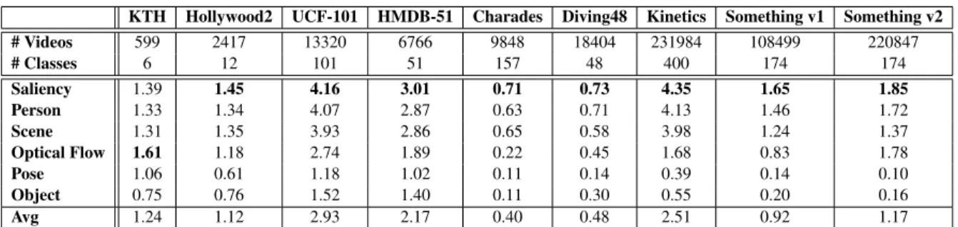
Table 2.1: Representation bias of the various datasets.
KTH Hollywood2 UCF-101 HMDB-51 Charades Diving48 Kinetics Something v1 Something v2
# Videos 599 2417 13320 6766 9848 18404 231984 108499 220847 # Classes 6 12 101 51 157 48 400 174 174 Saliency 1.39 1.45 4.16 3.01 0.71 0.73 4.35 1.65 1.85 Person 1.33 1.34 4.07 2.87 0.63 0.71 4.13 1.46 1.72 Scene 1.31 1.35 3.93 2.86 0.65 0.58 3.98 1.24 1.37 Optical Flow 1.61 1.18 2.74 1.89 0.22 0.45 1.68 0.83 1.78 Pose 1.06 0.61 1.18 1.02 0.11 0.14 0.39 0.14 0.10 Object 0.75 0.76 1.52 1.40 0.11 0.30 0.55 0.20 0.16 Avg 1.24 1.12 2.93 2.17 0.40 0.48 2.51 0.92 1.17
dataset [SZS12]. Given the optical flow maps, batches of 10 consecutive flow images, temporally separated by a stride of 10, are fed to the network. The implementation is based on [WXWQ15]. The output of the feature extraction stage of this network defines the optical flow representation, denotedφf low.
Pose bias- The fifth representation captures human pose. The feature extractor is the real-time multi-person 2D pose estimation algorithm of [CSWS17]. The frames are first sampled from the original video using a stride of 10 frames. The algorithm then extracts the pose of every person and represents it as an 18-joint skeleton. For each frame, a pose skeleton is chosen randomly and the x-y coordinates of each of the joints are concatenated. These concatenated coordinate vectors are used as pose features, defining the pose representationφpose.
Object bias- The final representation is based on object detection results produced by the Faster RCNN of [RHGS15]. This model is pre-trained on the 80 object classes of the MS-COCO dataset [LMB+14]. For each frame, objects corresponding to the top 5 classification scores are selected. The bounding box information of these detections along with their classification scores are then concatenated and used as object features, defining the object representationφob ject.
Bias measurements Given a representation φ, the corresponding feature extractor is used to
extract feature vectors from the training set of
D
. These are fed to a linear classifier which is then trained with respect to the classes ofD
. Next, the classifier is applied to the test set ofD
and the average precision of each class and its mean are recorded. This is the measure of performance2.2.4
Algorithms
While the study of bias is important, it is also interesting to understand how bias affects the performance of different algorithms. In its largest generality, this is a daunting task, since there are many action recognition algorithms and these can be quite complex. Running a large number of algorithms on a large number of datasets is beyond the reach of our computational capabilities, at the moment. However, many algorithms are variants or combinations of simpler
prototypicalalgorithms. Understanding how bias affects these algorithms provides insight on how it may affect the more complex variants. In this study, we considered the following prototypical algorithms. In all cases, we used a ResNet101 with the weights pretrained on ImageNet and finetuned on each dataset.
C2D-Spatial consists of the spatial stream of a Two-Stream CNN, implemented in isolation, by simple addition of a softmax layer to the C2D-Spatial feature extractor. To classify a video,
n frames are randomly selected from it, fed through the network, and the output class scores averaged. We usedn=3 for training andn=19 for inference. The training strategy is as per [SZ14], [WXWQ15] and [MCKA17].
C2D-Motionconsists of the temporal stream of the Two-Stream CNN, implemented in isolation, as above. The network processes stacks of 20 optical flow maps (10 channels each ofxandy
motion components). For training, we randomly pass just one of these stacks, for inference, 19 stacks are uniformly segmented and softmax outputs averaged.
C2D-Two Streamaverages the video-level predictions of the two models described above. Thus, this algorithm models the combination of static and dynamic features in a video.
Inflated 3D (I3D)-Spatialis the algorithm of [CZ17]. It consists of a 3D ConvNet which is the
inflatedversion of the 2D Inception-v1 network [IS15]. The feature extractor takes in segments of 64 consecutive RGB video frames in order to produce a feature vector. For training, one segment is randomly chosen from each video while for inference, 10 uniformly distributed segments are passed into the network and the outputs are averaged. The model we used has been pretrained on
ImageNet and then fine-tuned on the Kinetics dataset, as well as on each of our datasets.
P-CNN[CLS15] is similar to the two stream network, but with the additional guidance of pose-joint locations. In both spatial and motion streams, image patches containing parts of the human body (e.g. right and left hand) are passed through the CNN, producing initial image features, which are then aggregated asstaticanddynamicfeatures of corresponding body parts. Finally, they are concatenated into a single video feature vector. A linear SVM classifier is used for the final video classification.
2.3
Experiments
The representations and algorithms discussed above were used to perform a large number of experiments, whose results we describe in this section.
2.3.1
Representation bias
DatasetsWe started by characterizing the representation bias of 9 datasets. Table 2.1 gives the
information regarding the number of videos and classes present in each of the datasets evaluated in the thesis. The train/test splits we used is the same as those reported in the respective sources of the datasets.
Bias Table 2.1 summarizes the biases of all datasets for all representations. A number of observations can be made from the table. First, all datasets other than KTH have largest bias for the saliency representation. This is likely because most action datasets tend to involve object interactions. Understanding these interactions frequently requires a close-up view of the objects. This explains the dominance of the saliency bias. On the other hand, many of these objects tend not to belong to the classes detected by the Faster RCNN. This suggests that they are not ”popular” objects, which explains the low object bias. Second, comparing the datasets, it can be seen that UCF101 has the most average bias, while Charades and Diving48 have the least. This
can be explained by the fact that Charades contains lengthy videos with more than one label per video. Moreover, the labels are also quite different from one another - such as”Looking outside the window”combined with”Someone is cooking something”. As for the Diving dataset, the information within each frame is quite limited due to the similar environment and the objects related to the diving actions, which lowers down the biases from the static representations.
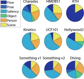
Figure 2.1: Dominant representation bias
Bias dominance: To obtain a more detailed picture of the bias within each dataset, we next performed an analysis of class bias. The pie-charts of Figure 2.1 illustrate the distribution of the class-level dominant representation bias for each of the datasets. They were obtained by identifying the strongest bias for each class, which is denoted thedominantbias, and counting the occurrences of these dominant biases across classes. A few conclusions can be taken from the figure. First, saliency bias is dominant for most datasets other than KTH. This agrees with the observations of Table 2.1. Second, the detailed picture is more nuanced than the broad picture painted by the table. While it is true that saliency usually dominates, this dominance has a large variation of intensity across datasets. On Kinetics and UCF101, saliency is dominant for more than half of the classes in the dataset. On the other hand, for Charades and Diving the saliency
slice is not much larger than some of the other slices.
Third, the second most dominant bias is, for most datasets, optical flow. The exceptions are again Kinetics and UCF101. This suggests that these datasets are heavily biased towards static representations. Among the remaining ones, Something-Something V2 and Diving have the best balance between static and dynamic biases. On the other hand, KTH is heavily biased to optical flow. Fourth, most datasets have very small bias towards object pose, which is explained by the limited vocabulary of the Faster RCNN, and zero pose bias. This suggests that body configurations do not play a major role in discriminating the action classes of these datasets. Exceptions are Charades and Diving, which are composed of actions of people doing things and athletes performing olympic dives. Finally, most datasets have a non-trivial amount of person bias. This is expected, since most actions involve humans. An important point to note here is that Figure 2.1 is also a reflection of the fairness score of a dataset
D
since it shows the distribution of the dominant class bias across the entire dataset. Thus, in this case, Charades and Diving are the mostfairdatasets since they have an almost uniform distribution among all the representations, while KTH is the most unfair.1.5 2 2.5 3 3.5 4 4.5 5 5.5 6
a - Strength of largest bias
0 0.005 0.01 0.015 0.02 0.025 0.03 0.035
b - rate of bias decay
UCF101 HMDB51 KTH Charades Kinetics Hollywood2 Something v1 Something v2 Diving
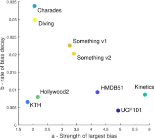
Figure 2.2: Characterization of bias skew of all datasets for saliency
biased or contain a ”bias skew,” i.e. a small percentage of very biased classes and a long tail of unbiased ones. For each dataset and representation, we sorted the classes by descending bias and fit an exponential decay law, of the form
B
ic=aie−bic, whereB
icis the bias of the class of rank cfor representationi, to the resulting raked bias values, by least squares. The parameteraiis ameasure of the strength of the largest bias for representationiin the dataset, whilebiencodes the rate of bias decay, capturing how quickly the bias falls across the sorted classes. The scatter plot of Figure 2.2 depicts the values of largest bias (a) vs. bias decay (b) of the different datasets for the saliency representation (φsal). Charades and Diving have small maximum bias that decays
very quickly. This is ideal behavior. On the other hand, UCF and Kinetics have large maximum bias, which decays slowly. This explains why these datases are so biased for saliency in Table 2.1. The remaining datasets ”interpolate” between these two behaviors, with the exception of KTH and Hollywood2. These outliers have both small maximum bias and small decay. For KTH, this is explained by fact that it has very little bias for saliency, as shown by the pie chart of Figure 2.1. Hollywood2 is a more interesting case. While bias for the saliency representation is dominant in many classes (Figure 2.1), the bias distribution is quite uniform across classes.
UCF101 HMDB51 KTH Charades Kinetics Hollywood2 Something v1 Something v2 Diving 1 2 3 4 5 6
a - Strength of largest bias
Pose UCF101 HMDB51 KTH Charades Kinetics Hollywood2 Something v1 Something v2 Diving 1 2 3 4 5 6
a - Strength of largest bias
Pose
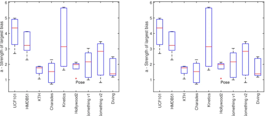
Figure 2.3: Box-plots of the strength of largest bias (”a”) and the rate of bias decay (”b”) for different datasets
Figure 2.3 summarizes the average and spread of thea-bvalues of each dataset across representations using a boxplot. With regards to the maximum biasa, UCF101 and HMDB51
have the highest median, while Kinetics has, by far, the largest range of values. This shows that the largest class bias is extremely strong for some representations. On the other hand, Charades and Diving have the smallest median max class bias. Regarding bias decay Charades has the largest median rate, indicating that it has the most skewed bias distribution. It is also interesting to note that the v2 for Something-Something has a greater median max bias athan v1 and an equivalent median decay rateb. This implies that the bias distribution of v2 upper bounds that of v1, and could be due to the different levels of granularity of the two datasets - more fine-grained action categories in v2, and even more fine-grained labeling via video captions as reported in [MBG+18]. Overall, Charades and Diving tend to have low and high values of ”a” and ”b” respectively, indicating that they have both a low overall bias and a low population of very highly biased classes.
Class Frequency
Average Class Bias
Correlation Coefficient = 0.0073
Class Frequency
Fairness Score
Correlation Coefficient = 0.1284
Figure 2.4: Correlation coefficients for average class bias and fairness score versus class frequency
Relations:We next considered whether bias and unfairness can be explained by dataset unbalance, i.e. unevenness of the class frequencies fi. Figure 2.4 presents a scatter plot of the average bias of each class vs. its frequency and a similar plot for the fairness scores. The two plots show very weak correlation between either of the bias properties and class frequency. This is positive, because action recognition datasets tend to be unbalanced, just due to the fact that it is easier to find videos of some actions than of others. These plots suggest that dataset unbalance is not a
major reason of concern, when it comes to representation bias. On the other hand, it would be much easier to correct representation bias if it were mostly due to class inbalance. The fact that this is not the case, suggests that further studies like the one we conducted are likely to be needed, as well as algorithms that specifically target bias removal.
2.3.2
Effect of bias on algorithms
Beyond characterizing the representation bias of datasets, we investigated how this bias affects algorithms.
Dependencies: We started by investigating how the different algorithms leverage the various biases present in a dataset. For this reason, we computed the bias of a dataset
D
towards each algorithmA
i by definingB
c(D
,A
i)to be the normalized (by fi) average precision ofA
itowards classc. In this way, we generalize the concept of bias calculation of a dataset towards both representations and algorithms. Thus, for a dataset such as HMDB51, we end up getting the matrix
B
(D
,A
)of size 51x5 comprising of the bias of each of the 51 classes towards our 5 algorithms.Representation/Algorithm similarity: The computation of the representation
B
c(D
,φi)and algorithmic
B
c(D
,A
j)biases, places algorithms and representations in a common space of dimension equal to the number of classes in the dataset. PCA was used to project this space on a 2D plane for visualizing the relationship between algorithms and representations. This helps to establish the kind of representations different algorithms favour. It can also be used to evaluate which algorithms might perform better on a new dataset, depending on the dominant representation bias it has.From (2.1), we already have the bias of the classes towards the 6 representations. This results in a matrix
B
(D
,φ)of size 51x6 for HMDB51. By concatenatingB
(D
,φ)andB
(D
,A
),we get 11 vectors, each of 51 dimensions. These vectors are then projected onto the space of the two largest principal components. This is given by Figure 2.5. There are a few notable
observa-Principal Component 1 Principal Component 2 Saliency Scene Person Pose Object Optical Flow C2D-Spatial C2D-Motion C2D-Two Stream I3D-Spatial P-CNN Representations Algorithms
Figure 2.5: PCA visualization of the algorithms and representations projected onto the space of the two largest Principal Components
tions here. Firstly, the C2D-Spatial as well as the I3D-Spatial algorithms lie close to the static representations while the C2D-Motion and PCNN are closer to the dynamic representation,φf low
and pose joint representation, φposerespectively. Secondly, it is intuitive to see that C2D-Two
Stream, which is the combination of the Spatial and Motion C2D algorithms, indeed lies around the middle. Thirdly, the Object representation,φob ject, is located far away from all the algorithms.
It shows that there are not a lot of action recognition algorithms which consider just object locations for classification purpose. This is in contrast to the Saliency representationφsal, which
is close to multiple algorithms. Thus, this result highlights the importance of object saliency over just its location.
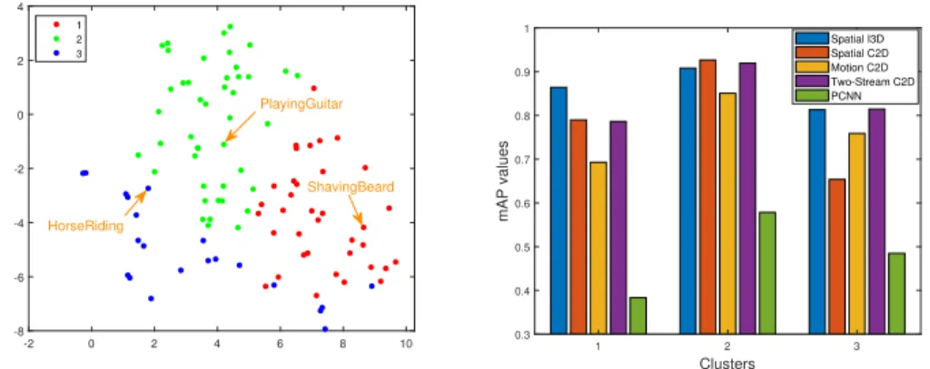
Bias-based Clustering analysis: One of the primary objectives of the work done here is to look deeper at a dataset in order to find similarities in its constituent classes in terms of bias. This motivates the idea of grouping orclusteringthe classes of a dataset according to the representation bias values and visualizing the performance of each cluster. This is shown in Figure 2.6. On the left side, we have the t-SNE plot [MH08] depicting 3 clusters of the UCF101 classes found according to the k-means clustering algorithm. The performance of the 5 algorithms
-2 0 2 4 6 8 10 -8 -6 -4 -2 0 2 4 1 2 3 PlayingGuitar HorseRiding ShavingBeard 1 2 3 Clusters 0.3 0.4 0.5 0.6 0.7 0.8 0.9 1 mAP values Spatial I3D Spatial C2D Motion C2D Two-Stream C2D PCNN
Figure 2.6: t-SNE visualization of clusters of UCF101 classes and the corresponding algorithm performance on each cluster
are then plotted on the right side for each of these clusters. It is observed that while the overall performance of C2D-Spatial is better than C2D-Motion for UCF101, this is not the case for cluster 3. This is possibly due to the presence of classes with short-term motion (such asHorseRiding). On the contrary, for cluster 2, the C2D-Spatial actually performs better than both the Two-Stream as well as I3D algorithms. This is a striking observation since I3D usually outperforms most C2D algorithms by a long margin [CZ17] .
2.3.3
Effect of Dataset Manipulation on Algorithms
The above sections mention the performance of thecompletedataset towards different representation biases and algorithms. Here, we introduce a novel technique of manipulating a dataset according to bias, in order to see a change in the performance of algorithms. During our implementation, the Spatial stream of C2D outperformed the Motion stream for UCF101. From Figure 2.5, it can be seen that the spatial algorithms rely more onφsal while the motion algorithm
on φf low. This is understandable since the former focus more on the static features while the
latter on short-term dynamics. Thus, theoretically, removing the classes according toφsal should
have some negative impact in the performance of the spatial algorithms. In our experiment, we therefore picked only the high-biased classes such as PlayingPiano, Skijetetc. (as shown in
Figure 1.1) which also have relatively low bias for φf low and recomputed the performance of
each of these algorithms.
0 1 3 5 7 9 11 13
Number of Classes Removed 80 80.5 81 81.5 82 82.5 83 Accuracy Spatial C2D Motion C2D Difference 1.5 1.25 1.0 0.75 0.5 0.25 0.0
Figure 2.7: Performance of two algorithms on UCF101 and their differences, with biased classes removed.
This is reflected in Figure 2.7 for the different number of classes removed. The curve overlaid on the bins denotes the difference in accuracy of the spatial and motion algorithms. Clearly, the difference decreases with the number of classes removed. This suggests that a simple manipulation of classes may indeed change/alter the performance of algorithms. This is an interesting result since it shows that relative algorithm performances are affected by the biases of the dataset. This is important, due to the prevalence of the ”state of the art” standard in the evaluation of vision algorithms. This practice encourages the promotion of algorithms that could be best at leveraging representation biases of the dataset, instead of solving the actual task. To make matters worse, datasets collected using similar data collection set-ups are likely to exhibit similar biases. For example, many data collection efforts use the same source (YouTube) and similar protocols (Turk annotations, etc.). While most recent efforts have focused on collecting
2.4
Conclusion
In this chapter, we studied different types of representation biases on most state-of-the-art action recognition datasets and found that they vary a lot with respect to different representations. A new metric, the fairness score, was also introduced to assess a dataset based on bias, and it was further proven that both this metric and the average bias of a dataset is uncorrelated with class frequency. We further established that the concentration of high-biased classes vary among datasets and this information can be utilized to reduce the overall bias of the dataset. The second part of the chapter rounds up the state-of-the-art algorithms and their relationship with different representations. We proved that algorithms tend to perform better in the presence of their preferred representations. Thus, when a new action recognition dataset is introduced, the optimal algorithm can be found based on this dataset’s bias. Finally, we showed that an algorithm’s performance is subject to the classes it is exposed to. Therefore, by removing biased classes of a dataset, it is totally possible to change or even alter the relative performance of different algorithms.
Chapter 3
Diverse Scene Detection
3.1
Background
Semantic place categorization using only visual features has been an important area of research for robotic applications [TMFR03, WCR09]. In the past, many robotics researchers focused on place recognition tasks [PMC08, SI07] or on the problem of scene recognition in computer vision [OT01, QT09].
Quattoni and Torralba [QT09] introduced a purely vision-based place recognition system, which improves the performance of the global gist descriptor by detecting prototypical scene regions. However, the size, shape and location of up to ten object prototypes has to be labeled and learned in advance for this system to work. Also, the labeling task is very work-intensive, and the approach of having fixed regions is only useful in finding objects in typical views of the scene. This makes the system ill-suited for robotics applications. Since we want to deal with flexible positions of objects, we apply a visual attention mechanism that can locate important regions in a scene automatically.
A number of different approaches have been proposed to address the problem of classify-ing environments. One popular approach adopted is to use Feature Matchclassify-ing with Simultaneous
Localization and Mapping (SLAM). Ekvallet al. [EKJ07] and Tonget al. [TSY17] demonstrated a strategy for integrating spatial and semantic knowledge in a service environment using SLAM and object detection & recognition based on Receptive Co-occurrence Histograms. Espinaceet al. [EKSR10] presented an indoor scene recognition system based on a generative probabilistic hi-erarchical model using the contextual relations to associate objects to scenes. Kollaret al. [KR09] utilize the notion of object-object and object-scene context to reason about the geometric structure of the environment in order to predict the location of the objects. The performance of the object classifiers is improved by including geometrical information obtained from a 3D range sensor that facilitates a focus of attention mechanism, in addition. However, these approaches only identify the place based on the specific objects detected and the hierarchical model that is used to link the objects with the place. In contrast to their method, our algorithm is not limited to a small number of recognizable objects.
Recently, there have been several approaches to Scene Recognition using Neural Networks. Liaoet al. [LKW+16, LKW+17] used Convolutional Neural Networks (CNNs) to recognize the environment based on object occurrence for semantic reasoning, but their system information and mapping results are not provided. Sunet al. [SMTA18] proposed a Unified Convolutional Neural Network which performs Scene Recognition and Object Detection. Luoet al. [LC18] developed a semantic mapping framework utilizing spatial room segmentation, CNNs trained for object recognition, and a hybrid map provided by a customized service robot. Nikoet al. [SDM+16] proposed a transferable and expandable place categorization and semantic mapping system that requires no environment-specific training. Mancini et al. [MBCR18] addressed Domain Generalization (DG) in the context of semantic place categorization. They also provide results of state-of-the-art algorithms on the VPC Dataset [WCR09] that we compare to. However, most of these results do not test their algorithms on a wide variety of platforms. This is the main focus of the work shown in this chapter. The experiments are conducted, both for static images, and dynamic real world videos captured using hand-held cameras and robots.
3.2
Proposed Methodology
We consider a set of five different models, abbreviated as Diverse scEne Detection methods in Unseen Challenging Environments (DEDUCE), for place categorization. Each model is derived from two base modules, one based on the PlacesCNN [ZLK+17] and the other being an Object Detector-YOLOv3 [RF18]. The classification model can be formulated as a supervised learning problem. Given a set of labeled training data
X
tr={(x1,y1),(x2,y2)...(xN,yN)}, wherexi corresponds to the data samples andyi to the scene labels, the classifier should learn the
discriminative probability model
p(yˆj|Φ(
X
tr)) (3.1)where ˆyjcorresponds to the j-th predicted scene label andΦ={φ1,φ2...φt}are the set of different
feature representations obtained from the xi. This trained model should be able to correctly
classify a set of unlabelled test samples
X
te={x1,x2...xM}. It is to be noted that while the goalof each of our five models is to perform place categorization, it is theΦwhich varies across them.
We now describe the two base modules, and how our five models are derived and trained from them. The complete network architecture is given in Figure 3.1.
0 0 .. . FC Bedroom YOLOv3 Input Image Hot-encoded vector Scene_only Object_only Combined 1 PlacesCNN Kitchen Living Room Dining Room Office
Figure 3.1: Model Architecture. The highlighted regions represent the portion of the network which was trained for the respective models.
3.2.1
Scene Recognition
For scene recognition, we use the PlacesCNN model. The base architecture is that of Resnet-18 [HZRS16] which has been pre-trained on the ImageNet dataset [DDS+09] and then fine-tuned on the Places365 dataset [ZLK+17]. We choose seven classes out of the total 365 classes, which are integral to the recognition of indoor home/office environments - Bathroom, Bedroom, Corridor, Dining room, Living room, Kitchen and Office. We use the official training and validation split provided for our work. The training set consists of 5000 labelled images for each scene-class, while the test set contains 100 images for each scene.
3.2.2
Object Detection
Object detection is a domain that has benefited immensely from the developments in deep learning. Recent years have seen people develop many algorithms for object detection, some of which include YOLO [RDGF16, RF17, RF18], SSD [LAE+16], Mask RCNN [HGDG17], Cascade RCNN [CV18] and RetinaNet [LGG+17]. We work with the YOLOv3 [RF18] detector here, mainly because of its speed, which makes real-time processing possible. It is a Fully Con-volutional Network (FCN), and employs the Darknet-53 architecture which has 53 convolution layers, consisting of successive 3x3 and 1x1 convolutional layers with some shortcut connec-tions. The network used here has been pre-trained to detect the 80 classes of the MS-COCO dataset [LMB+14].
3.2.3
Place Categorization models
Scene OnlyThe first model which we use consists of only the pre-trained and fine-tuned PlacesCNN with a simple Linear Classifier on top of it. This model accounts for a holistic representation of a scene, without specifically being trained to detect objects. Thus, the feature vector for this model
is given byΦscene=φs.
Object Only
The second model acts a Scene classifier using only the information of detected objects. There is no separate training performed here to identify the individual scene attributes. For this purpose, we create a codebook of the most common COCO-objects seen in all the seven scenes. This is shown in Table 3.1. It is to be noted that every object has been associated to only one scene, thereby making it alandmark. For this model, the feature representation is given byΦob j=φ{ob j}
where{ob j}is the set of objects detected in the image.
Table 3.1: Top landmark objects (non-human) for the seven different scene classes
Bathroom Toilet Sink -
-Bedroom Bed - -
-Corridor - - -
-Dining Room Dining Table Chair Wine Glass Bowl
Kitchen Oven Microwave Refrigerator
-Living Room Sofa Vase -
-Office TV-Monitor Laptop Keyboard Mouse
Scene+Attention
In this model, we compute the activation maps for the given image of a scene, and using those, we try to visualize where the network has its focus during scene classification. From the output of the final block convolutional layer (layer 4) of the WideResnet architecture [ZK16], we get the 14x14 feature blobs which retain the spatial information corresponding to the whole image. Our model is similar to thesoftattention mechanism of [XBK+15] in the sense that here too, we assign the weights to be the output of a softmax layer, thereby associating a probability distribution to it. However, since we are not classifying based on a sequence of images, we do not employ a recurrent network to compute the sequential features. Instead, we simply utilize the weights of the final FC layer and take its dot product with the feature blobs to obtain the
heatmap. The final step is to upsample this 14x14 heatmap to the input image size, and then overlay it on top to obtain the activation maskm(xn)of the input imagexn. Therefore, the feature representation for this model isΦattn.=φm(xn). The basic architecture is given in Figure 3.2.
14 x 14 Feature Map
Input Image PlacesCNN Activation Map
Figure 3.2: Architecture for Generation of the Activation Map. The 14x14 feature maps obtained from the block layer 4 of WideResNet are combined with the weights from the final FC layer, and then their dot product id upsampled to the image size and overlaid on top to get the activation maps
Combined
In this model, we use the PlacesCNN mentioned above as a feature extractor to give the semantics of a scene. In addition, the YOLO detector gives us the information regarding the objects present in the image. Given an image of a scene, our model creates a hot-encoded vector of 80 dimensions, corresponding to the object classes of MS-COCO, with only the indices of the detected objects set to 1. We then concatenate this vector along with that of the output of the scene feature extractor, and train a Linear Classifier on top of it. Since we combine the two different features of scene and objects, the feature representation here is given byΦcomb.={φs,φ{ob j}}.
Scene+N-best objects
Our final model is similar to the above in the sense that here also, we use both the PlacesCNN and the YOLO detector. However, this model does not need to be retrained again and so, it is significantly faster. For this model, we place a certain confidence threshold on the scene detector, and only when the probability of classification is below this threshold, we search
for the information about specific objects in the scene (as obtained from Table 3.1). The reason for introducing this as a new model is two-fold. Firstly, we eliminate the scenario of looking at every object present since it is often redundant, given the semantics of the scene. Secondly, this is similar to how we as human beings operate when we come across an unknown scene. The feature representation for this model is given byΦN−best ={φs,φ{N−ob j}}.
3.3
Experiments and Results
We evaluated our five models described above on a number of platforms. In this section, we first describe our training procedure, and then talk about the different experiment settings used for evaluation.
3.3.1
Training Procedure
As mentioned in Section 3.2, the base architecture for our scene classifier is the ResNet-18 architecture. The data pre-processing and training process is similar to [ZLK+17]. We used the Stochastic Gradient Descent (SGD) optimizer with an initial learning rate of 0.1, momentum of 0.9, and a weight decay of 10−4. For theΦsceneand theΦattn.models, the training was performed
for 90 epochs with the learning rate being decreased by a factor of 10 every 30 epochs. The
Φcomb.model converged much faster and so, it was only trained for 9 epochs, with the learning
rate reduced by 10 times after every 3 epochs. For all the 3 training procedures, the cross-entropy loss function was optimized, which minimizes the cost function given by
J(yˆj,yj) =−1 N( N
∑
j=1 yjlog(yˆj)) (3.2)The training process was carried out on a NVIDIA Titan Xp GPU using the PyTorch framework. The performance of the five DEDUCE algorithms on the test set of Places365 is
shown in Table 3.2 for the seven classes chosen.
Table 3.2: Accuracy in percentage of DEDUCE on Places365 dataset
Scenes Φscene Φob j Φattn. Φcomb. ΦN−best
Dining room 79 94 75 79 80 Bedroom 90 74 90 90 91 Bathroom 92 65 92 91 92 Corridor 94 90 99 96 94 Living Room 84 25 68 80 84 Office 85 29 76 94 83 Kitchen 87 62 70 87 87 Avg 87.3 62.6 81.4 88.1 87.3
3.3.2
Experiment Settings
In order to check the robustness of our models, we further evaluated their performance on two state-of-the-art still-image datasets.
SUN Dataset
The SUN-RGBD dataset [SLX15] is one of the most challenging scene understanding datasets in existence. It consists of 3,784 images using Kinect v2 and 1,159 images using Intel RealSense cameras. In addition, there are 1,449 images from the NYUDepth V2 [SHKF12], and 554 manually selected realistic scene images from the Berkeley B3DO Dataset [JKJ+13], both captured by Kinect v1. Finally, it has 3,389 manually selected distinguished frames without significant motion blur from the SUN3D videos [XOT13] captured by Asus Xtion. Out of this, we sample the seven classes of importance and use the official test split to evaluate our models. We only consider the RGB images for this work since our training data doesn’t have depth information. The performance is summarized in Table 3.3.
Upon comparison with Table 3.2, which contains the results on the Places365 dataset where our models were fine-tuned, a number of observations can be made which are consistent for both the datasets. Firstly, theΦcomb. model performs the best. This is intuitive since here,
Table 3.3: Accuracy in percentage of DEDUCE on SUN dataset
Scenes Φscene Φob j Φattn. Φcomb. ΦN−best
Dining room 65.2 83.7 53.3 67.4 72.8 Bedroom 43.7 36.5 48.9 48.9 47.3 Bathroom 94.5 87.0 97.3 96.6 95.2 Corridor 44.4 67.6 67.6 44.4 41.7 Living Room 58.8 24.0 43.6 59.2 58.8 Office 84.0 12.6 75.8 90.6 80.6 Kitchen 77.1 63.5 63.9 83.8 77.4 Avg 66.8 53.6 64.3 70.1 67.7
the scene classification is done using the combined training of both the information about the scene attributes and the object identity. Secondly, theΦob j model works the best for theDining Roomclass, even though its overall performance is the worst. This trend can be attributed to the fact that dining rooms can be easily identified by the presence of specific objects, whereas the scene attributes might throw in some confusion (for instance when the kitchen/living room is partially visible in the image of a dining room). Thirdly, forCorridor, the performance of the
Φattn.model is best for both the datasets. This supports the fact that in order to classify a scene
like a corridor, viewing only a small portion of the image close to the vanishing point is sufficient. Finally, theΦN−best model performs just as good or better than theΦscene model. This proves
that presence of objects does indeed improve the scene classification. For the best performance using theΦN−best model, the threshold was set to 0.5 for thePlacesdataset while it was 0.6 for
theSUN dataset. The reason for the higher confidence on scene attributes forPlacesdataset is most likely due to the fact that the scene classifier itself was fine tuned on it.
VPC Dataset
The Visual Place Categorization dataset [WCR09] consists of videos captured autonomously using a HD camcorder (JVC GR-HD1) mounted on a rolling tripod. The data has been collected from 6 different home environments, and three different floor types. The advantage of this dataset is that the collected data closely mimics that of the motion of a robot - instead of focusing on
captured frames or objects/furniture in the rooms, the operator recording the data just traversed across all the areas in a room while avoiding collision with obstacles. For comparison with the state-of-the-art algorithms, we test our methods only on the five classes which are present in all the homes - Bathroom, Bedroom, Dining room, Living room and Kitchen. Table 3.4 contains the results for the individual home environments for these five classes. For the AlexNet [KSH12] and ResNet [HZRS16] models, we adopt the same training procedure as in [MBCR18]. It can be seen from the table that our models perform better than the rest in all but one of the home environments and much better in the overall performance.
Table 3.4: VPC Dataset: Average Accuracy across the 6 home environments
Networks H1 H2 H3 H4 H5 H6 avg. AlexNet 49.8 53.4 49.2 64.4 41.0 43.4 50.2 AlexNet+BN 54.5 54.6 55.6 69.7 41.8 45.9 53.7 AlexNet+WBN 54.7 51.9 61.8 70.6 43.9 46.5 54.9 AlexNet+WBN∗ 53.5 54.6 55.7 68.1 44.3 49.9 54.3 ResNet 55.8 47.4 64.0 69.9 42.8 50.4 55.0 ResNet+WBN 55.7 49.5 64.7 70.2 42.1 52.0 55.7 ResNet+WBN∗ 56.8 50.9 64.1 69.3 45.1 51.6 56.5 Ours (Φscene) 63.7 57.3 63.7 71.4 60.2 65.9 63.7 Ours (Φcomb.) 63.7 60.7 64.5 70.7 65.7 68.8 65.7
Table 3.5 further compares our models with all other baseline algorithms tested on the VPC dataset. The reported accuracies are the average over all the six home environments. We first consider the methods described in [WCR09], which use SIFT and CENTRIST features with a Nearest Neighbor Classifier, and also exploit temporal information between images by coupling them with Bayesian Filtering (BF). Next, we look at the approach of [FET12] where Histogram of Oriented Uniform Patterns (HOUP) is used as input to the same classifier. [YW12] proposed the method of using object templates for visual place categorization, and reported results
Table 3.5: VPC Dataset: Comparison with State Of The Art
Method [WCR09] [FET12] [YW12] AlexNet ResNet Ours
Config. SIFT SIFT+BF CE CE+BF HOUP G+BF G+O(SIFT)+BF Base BN WBN∗ BN WBN∗ Scene-only Combined
for Global configurations approach with Bayesian Filtering (G+BF), and that combined with the object templates (G+O(SIFT)+BF). Ushering the deep learning era, AlexNet [KSH12] and ResNet [HZRS16] architectures give better results, both with their base models, as well as the Batch Normalized (BN) and the Weighted Batch Normalized versions [MBCR18]. However, comparisons with ourΦsceneandΦcomb.models show that our methods beat all the other results
by significant margins.
Figure 3.3: Detection Results on Real-World Videos. Top row corresponds to the video of a Real-Estate model house. The next 2 rows are from the houses of the authors and their friends. The bottom row is obtained from a house in the movie”Father of the Bride”.
Real-World Scene Recognition
In order to test the robustness of our DEDUCE models, we expand the domain of test cases beyond the aforementioned still image data sets. Figure 3.3 does this by showing the results of scene recognition on real-world data recorded using hand-held cameras. We employ the
ΦN−best model for these cases due to its ability to mimic the natural behavior of humans, whereby
an initial prediction is made based on the scene attributes, and if unsure, more information related to specific objects is g