UC San Diego
UC San Diego Electronic Theses and Dissertations
TitlePrimal-Dual Path-Following Methods For Nonlinear Programming Permalink https://escholarship.org/uc/item/9wv1z3qw Author Su, Fangyao Publication Date 2019 Peer reviewed|Thesis/dissertation
UNIVERSITY OF CALIFORNIA SAN DIEGO
Primal-Dual Path-Following Methods For Nonlinear Programming
A dissertation submitted in partial satisfaction of the requirements for the degree Doctor of Philosophy in Mathematics by Fangyao Su Committee in charge:
Professor Philip E. Gill, Chair Professor Randolph E. Bank Professor Thomas R. Bewley Professor Hyunsun A. Kim Professor Jiawang Nie
Copyright Fangyao Su, 2019 All rights reserved.
The Dissertation of Fangyao Su is approved, and it is acceptable in quality and form for publication on microfilm and electronically:
Chair
University of California San Diego 2019
EPIGRAPH
I care not whether I can achieve, for the longed goal, I shall despite wind and rain go. —Guozhen Wang
TABLE OF CONTENTS
Signature Page . . . iii
Epigraph . . . iv
Table of Contents . . . v
List of Figures . . . vii
List of Tables . . . viii
List of Algorithms . . . ix
Acknowledgements . . . x
Vita . . . xi
Abstract of the Dissertation. . . xii
Chapter 1 Introduction . . . 1
1.1 Problem Description . . . 1
1.2 Contributions of This Dissertation . . . 3
1.3 Notation . . . 4
1.4 Some Useful Results . . . 4
Chapter 2 Background . . . 7
2.1 Optimality Conditions . . . 7
2.1.1 Optimality Conditions for (NEP) . . . 7
2.1.2 Optimality Conditions for (NIP) . . . 11
2.2 Newton’s Method and Line Search . . . 17
2.2.1 Newton’s Method . . . 17
2.2.2 Model-Based Line Search Methods . . . 19
Chapter 3 A Primal-Dual Path-Following Augmented Lagrangian Method 21 3.1 Introduction . . . 21
3.2 Background . . . 22
3.2.1 The Penalty Function Method . . . 22
3.2.2 Augmented Lagrangian Method . . . 28
3.3 Motivation of The Proposed Algorithm . . . 33
3.4 Description of the Proposed Algorithm . . . 35
3.4.1 Description of The Outer Iteration . . . 36
3.4.2 Description of the Inner Iteration . . . 39
3.5 Convergence Analysis . . . 44
Chapter 4 A Combined Trust-Region Line-Search Method . . . 51
4.1 Background on Trust-Region Methods . . . 52
4.2 A Combined Trust-Region Line-Search Method . . . 55
4.3 Convergence of the Trust-Region Method . . . 57
4.4 Computing a Trust-Region Step . . . 62
Chapter 5 A Primal-Dual Path-Following Shifted Penalty-Barrier Method 67 5.1 Introduction . . . 67
5.2 Background . . . 68
5.2.1 Conventional Barrier Method . . . 68
5.2.2 Modified Primal-Dual Interior Methods . . . 73
5.3 Description of the Proposed Algorithm . . . 79
5.3.1 Algorithm Overview . . . 79
5.3.2 Description of the Outer Iteration . . . 81
5.3.3 A Shifted Penalty-Barrier Merit Function . . . 83
5.3.4 Description of the Inner Iteration . . . 87
5.4 Convergence Analysis . . . 100
5.5 Acknowledgement . . . 111
Chapter 6 Numerical Implementations . . . 112
6.1 Numerical Results of Primal-Dual Path-Following Augmented Lagrangian Method . . . 114
6.2 Numerical Results of Primal-Dual Path-Following Shifted Penalty-Barrier Method . . . 117
LIST OF FIGURES
Figure 3.1 Level Curves of the Conventional Quadratic Penalty Function for Dif-ferent Values of µ . . . 27 Figure 3.2 Level Curves of augmented Lagrangian Function for Different Values of µ 32 Figure 3.3 Path-Following Trajectories of The Primal-Dual Path-Following
Aug-mented Lagrangian Method with Different Starting Points . . . 44 Figure 5.1 Feasible Region and Level Curves of Objective Function in HS22 . . . . 70 Figure 5.2 Level Curves of the Conventional Logarithmic Barrier Function in the
Feasible Region for Different Values of µ . . . 71 Figure 5.3 Feasible Region and Level Curves of the Modified Barrier Function with
the Barrier Parameter µ= 10−1 . . . 75 Figure 5.4 Different Path-Following Trajectories Starting From Either Feasible or
LIST OF TABLES
Table 6.1 Definition of the Headings in all Tables . . . 113
Table 6.2 Default Parameters Used in PDAL . . . 114
Table 6.3 Numerical Results of PDAL . . . 115
Table 6.4 Default Parameters Used in PDPB . . . 117
Table 6.5 Numerical Results of PDPB – With Trust-Region Method . . . 119
Table 6.6 Numerical Results of PDPB – With Combined Trust-Region Line-Search Method . . . 122
LIST OF ALGORITHMS
Algorithm 2.1 Conventional Newton’s Method . . . 17
Algorithm 2.2 A Model-based Line Search Method . . . 19
Algorithm 3.1 Conventional Quadratic Penalty Function Method . . . 26
Algorithm 3.2 Augmented Lagrangian Method for (NEP) . . . 31
Algorithm 3.3 Primal-Dual Path-Following Augmented Lagrangian Method . . . 38
Algorithm 4.1 Basic Trust-Region Method . . . 53
Algorithm 4.2 A Combined Trust-Region Line-Search Method . . . 56
ACKNOWLEDGEMENTS
First of all, I would like to express the deepest gratitude to my advisor, Professor Philip E. Gill for his constant encouragement and guidance, for passing his rigorous attitude as a mathematician to me, and for his knowledge, patience and support for me in all aspects over the past 5 years. As a world-leading expert in optimization, he leads me into this branch of mathematics that used to be totally fresh to me.
I would like to acknowledge Profs. Randolph E. Bank, Jiawang Nie for the knowledge they taught me in graduate classes at UCSD and Profs. Thomas R. Bewley, Hyunsun A. Kim for their time to serve as my committee member.
I am very grateful for Yuanjie Jiang for her love and encouragement, my parents for their unconditional support to my career and life. I would also like to thank my friends Dun Qiu, Xiudi Tang, Xuefeng Shen, Yi Luo, Zihao Li and David Lenz at UCSD for their discussions with me on math problems and my officemates Yesheng Huang, Yingjia Fu and Yucheng Tu for their help in all aspects.
Chapter 3, in part is currently being prepared for submission for publication of the material. Su, Fangyao; Gill, Philip E. The dissertation author was the primary investigator and author of this material.
Chapter 5, in part is currently being prepared for submission for publication of the material. Su, Fangyao; Gill, Philip E. The dissertation author was the primary investigator and author of this material.
VITA 2014 Bachelor of Science in Mathematics
University of Science and Technology of China 2015-2019 Teaching Assistant
University of California San Diego 2017-2018 Research Assistant
University of California San Diego 2019 Doctor of Philosophy in Mathematics
ABSTRACT OF THE DISSERTATION
Primal-Dual Path-Following Methods For Nonlinear Programming
by
Fangyao Su
Doctor of Philosophy in Mathematics University of California San Diego, 2019
Professor Philip E. Gill, Chair
The main goal of this dissertation is to study the formulation and analysis of primal-dual path-following methods for nonlinear programming (NLP), which involves the mini-mization or maximini-mization of a nonlinear objective function subject to constraints on the variables. Two important types of nonlinear program are problems with nonlinear equal-ity constraints and problems with nonlinear inequalequal-ity constraints. In this dissertation, two new methods are proposed for nonlinear programming. The first is a new primal-dual path-following augmented Lagrangian method (PDAL) for solving a nonlinear program with equality constraints only. The second is a new primal-dual path-following shifted penalty-barrier method (PDPB) for solving a nonlinear program with a mixture of equality and inequality constraints. The method of PDPB may be regarded as an extension of PDAL to handle nonlinear inequality constraints.
structure involving outer and inner iterations. In the outer iteration of PDAL, the optimality conditions are perturbed to define a “path-following trajectory” parameterized by a set of Lagrange multiplier estimates and a penalty parameter. The iterates are constructed to closely follow the trajectory towards a constrained local minimizer of the nonlinear program. If an outer iterate deviates significantly from the trajectory, then an inner iteration is invoked in which a primal-dual augmented Lagrangian merit function is minimized to force the iterates back to a neighborhood of the trajectory.
A similar approach is used to handle the inequality constraints in PDPB. In this case, the trajectory is followed towards a local solution of the mixed-constraint nonlinear program. This trajectory is parameterized by a set of Lagrange multiplier estimates and penalty and barrier parameters associated with the equality and inequality constraints. If an iterate moves away from the trajectory, a primal-dual shifted penalty-barrier merit function is minimized using a trust-region method. By introducing slack variables, global convergence can be achieved from any starting point without the need for an initial strictly feasible point. Furthermore, numerical experiments indicate that when minimizing the shifted barrier function, the trust-region method requires fewer matrix factorizations and iterations than a comparable line-search method.
Chapter 1
Introduction
1.1
Problem Description
In constrained optimization problems, the optimal value of objective function and its corresponding solution set must be found subject to certain constraints being satisfied. One of the most general formats used to express a nonlinear program is given by
minimize x∈Rn f(x)
subject to c` ≤ c(x)≤cu, x` ≤ x≤xu,
(1.1)
where f(x) :Rn 7→
R is the objective function and c(x) :Rn 7→ Rm are the constraints. c` and cu are the lower and upper bounds of c(x) in Rm, x` and xu are the lower and upper bounds of x in Rn. As maximizing f(x) is equivalent to minimizing −f(x), without loss of generality, only minimizing an objective function will be considered.
Problem (1.1) can be written in the following simpler equivalent format in which each constraint is expressed in terms of a single nonnegative function:
minimize
x∈Rn f(x) subject to c(x)≥0. (NIP)
Given a vectors of nonnegative slack variables, problem (NIP) can be written in the equivalent form minimize x∈Rn, s∈ Rm f(x) subject to c(x)−s= 0, s ≥0. (NIPs) A special case of the problems (NIP) and (NIPs) occurs when all the constraints are equalities. In this case the problem is
minimize x∈Rn
f(x) subject to c(x) = 0. (NEP) In general, problem (NEP) is easier to solve than problem (NIP) and has a number of useful properties. Chapter 3 starts with a proposed primal-dual path-following augmented Lagrangian method for problem (NEP) and then this method is extended with the barrier term introduced to deal with the inequality constraints in Chapter 5.
Common types of optimization problem include linear programming (LP), where both f(x) and c(x) are affine functions, and quadratic programming (QP) where f(x) is in quadratic form andc(x) is affine. Optimization problems may also be categorized in terms of the level of smoothness of the objective and constraint functions. This dissertation concerns the formulation and analysis of algorithms for problems in which f(x) and c(x) are twice continuously differentiable, nonlinear and nonconvex. In all cases it is assumed that the gradient and Hessian are available at any given point. Knowledge of the second derivatives allows the formulation of methods with a superlinear or quadratic rate of convergence to a solution.
Finally, only algorithms for finding local minimizers are considered in this disserta-tion.
1.2
Contributions of This Dissertation
In this dissertation, Chapter 2 serves as a general background for all the subse-quent chapters. In Chapter 3, a primal-dual path-following augmented Lagrangian method (PDAL) is proposed for solving problem (NEP). In this method, the optimality conditions are perturbed to define a path-following trajectory, and all the iterates are forced to follow it towards a local constrained minimizer of problem (NEP). Once some iterate departs from this trajectory, an augmented Lagrangian type merit function that measures the distance between current iterate and the trajectory will be minimized using line-search method.
Like many other primal-dual methods proposed by Gill and coauthors (see [10, 12, 18, 21]), the proposed algorithms treat both the primal and dual variables as independent variables at each iteration. This strategy is different from that of other methods that regard the dual variables as being dependent on the primal variables and update them each time the primal variables are modified. This can provide certain benefits, such as the ability to control the quality of the dual variables during the solution of each subproblem, and the ability to impose explicit bounds on the dual variables. These strategies can improve both the efficiency and the reliability of a method.
In Chapter 5, the method of PDAL is extended to solve problem (NIP). In this chap-ter, a new primal-dual path-following shifted penalty-barrier method (PDPB) is proposed with some features inherited from PDAL. In the inequality constrained case the algorithm follows a trajectory defined by perturbing the optimality conditions of problem (NIP). If an iterate departs from the trajectory, a modified penalty-barrier function is minimized using a combined trust-region line-search method. As in the case of algorithm PDAL, this strategy guarantees global convergence. Unlike PDAL where line-search techniques are used, PDPB is a trust-region method, which implies that unlike a line-search method, it is not neces-sary to use an inertia-controlling factorization of the Hessian of the Lagrangian function. Furthermore, it can be shown that when minimizing the shifted-barrier function, incorpo-rating a line-search technique into the trust-region method generally requires fewer matrix
factorizations and fewer iterations, which brings certain numerical benefits.
1.3
Notation
Most of notations in this dissertation are consistent with the standard optimization literature. f(x) specifically refers to the objective function with g(x) and H(x) being its gradient and Hessian. c(x) specifically refers to the constraint function with J(x) being its Jacobian matrix, whosei-th row is defined by ∇ci(x)T. The subscriptk means the function takes value at iteratexk, say, gk meansg(xk). I refers to identity matrix with its dimension inferred from the context. e is a vector of all ones and ei is the i-th column of identity matrix. For a symmetric matrix A, the inertia of A, denoted by In(A), is the 3-tuple (i+,
i−,i0) indicating the number of positive, negative and zero eigenvalues of A. The norm|| · ||
refers to vector 2-norm and its induced matrix 2-norm unless otherwise stated. x·y is the element-wise product of two column vectors such that [x·y]i = xiyi, similarly, min (x, y) is a vector with components min (xi, yi). The vector consisting of xaugmented byy is defined by (x, y). Given δ >0, an open ball atx∗ is denoted byB(x∗, δ) ={x:||x−x∗||< δ}. The
i-th eigenvalue of a matrixAis denoted by λi(A). Finally,H 0 andH 0 refer to matrix
H being positive semidefinite and positive definite respectively. The{Hk}k≥0 are said to be
uniformly positive definite if there exists some constant λ > 0 such that for all k ∈ N and allp∈Rn,pTH
kp≥λ||p||2. If there exists a positive constantγ such that||αj|| ≤γβj, then write αj =O(βj). If there exists a sequence {γj}j≥0 →0 such that ||αj|| ≤γjβj, then write
αj =o(βj).
1.4
Some Useful Results
In this section, some useful results will be described that will be used frequently without proofs throughout this dissertation.
Lemma 1.4.1 (Sylvester’s law of inertia). If K is symmetric, then In(XTKX) = In(K) for any nonsingular matrix X, where In(K) denotes the inertia of K, i.e., the number of positive, negative and zero eigenvalues of K.
Lemma 1.4.2 (Inertia of the KKT matrix I). Given an n×n symmetric matrix H and an
m×n matrix J, let r denote the rank of J and let Z ∈ Rn×m be a matrix whose columns span the null space of J. Consider a Karush–Kuhn–Tucker (KKT) matrix of the form
K = H JT J 0 .
Then the inertia of K is given by
In(K) = In(ZTHZ) + (r, r, m−r).
The matrix ZTHZ is known as the reduced Hessian and describes the curvature of objective function on the active constraint surface.
Lemma 1.4.3 (Inertia of the KKT matrix II). Given an n×n symmetric matrix H and an
m×n matrix J of rank m, let Z ∈Rn×m be a matrix whose columns span the null space of
J. If a KKT matrix K is given by K = H JT J 0 ,
then the inertia of K is given by
In(K) = In(ZTHZ) + (m, m,0).
If ZTHZ is positive definite, then In(K) = (n, m,0), in which case, the KKT matrix K is said to have the correct inertia.
Lemma 1.4.4 (Inertia of the KKT matrix III). Given an n×n symmetric matrix H and an m×n matrix J of rank r, let the n−r columns of Z define a basis for null(J) and define the regularized KKT matrix as
Kµ= H JT J −µI . (1.2)
If µ > 0 is sufficiently small, then the following statements are equivalent.
• H+µ1JTJ is positive definite.
• In(Kµ) = (n, m,0).
• ZTHZ is positive definite.
Proof. Use the Schur complement and Debreu’s Lemma, which is given below.
Notice that in Lemma 1.4.4, there is no need forJ to have full rank anymore, as long as µ > 0 sufficiently small and the reduced Hessian is positive definite, Kµ will have the correct inertia. The −µI term in (2,2) block is generally regarded as a regularization of the KKT matrix.
Lemma 1.4.5(Debreu’s Lemma). There exists a finiteρ >¯ 0such that H+ρJTJ is positive definite for all ρ≥ρ¯if and only if pTHp >0 for all nonzero p such that J p= 0.
The matrix Kµ in (1.2) represents a “general” form of KKT matrix, where (1,1) block represents the Hessian of Lagrangian function or its approximation and (1,2) block represents the Jacobian of the constraints with (2,2) block being 0 or some diagonal matrix. In the context of the augmented Lagrangian method or shifted barrier method, KKT matrix is generally much more complicated but shares the same structure with Kµ. Moreover, the techniques used to modify the inertia of matrix in the form ofKµ to solve the KKT system will also be frequently used in this dissertation.
Chapter 2
Background
This chapter provides some background results for the subsequent chapters. Sec-tion 2.1 introduces the optimality condiSec-tions and corresponding constraint qualificaSec-tions for both (NEP) and (NIP). Section 2.2 describes Newton’s method and the commonly used line-search strategies. The background of a conventional augmented Lagrangian method for (NEP), which is the basis of the proposed primal-dual path-following augmented La-grangian method, is considered in Chapter 3. Similarly, the first part of Chapter 5 describes the conventional barrier method for (NIP) that serves as a basis for the proposed primal-dual path-following shifted penalty-barrier method. Finally, the background theory of the combined trust-region line-search method used to minimize the primal-dual shifted penalty-barrier function is discussed in Chapter 4.
2.1
Optimality Conditions
2.1.1
Optimality Conditions for (NEP)
In this section the constraint qualifications and optimality conditions for a constrained local minimizer are provided for problem (NEP). First, the definition of a constrained local minimizer is given.
Definition 2.1.1 (Local minimizer). Let f(x) : Rn 7→
R be the objective function and let
F ={x:c(x) = 0}denote the feasible region. A point x∗ is a constrained local minimizer of
f(x) if x∗ ∈ F and there exists an open ball B(x∗, δ) such that
f(x∗)≤f(x)for allx∈ B(x∗, δ)∩ F.
Furthermore, x∗ is a strict constrained local minimizer if
f(x∗)< f(x)for allx∈ B(x∗, δ)∩ F, x6=x∗.
The point x∗ is an isolated constrained minimizer if there exists a positive δ such that x∗ is the unique constrained local minimizer in B(x∗, δ)∩ F.
Definition 2.1.2(Feasible path). Assume thatxis a feasible point, i.e., c(x) = 0. A feasible path is a twice continuously differentiable curve x(α) such that
• x(0) =x, c(x(α)) = 0 for all 0≤α <αˆ and some α >ˆ 0; and
• the tangent vector dαd x(α) is nonzero at α= 0.
Definition 2.1.3 (Level set and Level curves). Given a functionf(x) :D ∈ Rn 7→
Rdefined on a convex set D, the level set L(γ) associated with the scalar γ, is the set
L(γ) ={x∈ D :f(x)≤γ}.
The boundary of the level setL(γ), i.e.,{x∈ D :f(x) =γ}is called the level curve associated with γ.
Definition 2.1.4 (Lagrange multipliers). Assume that x∗ is a constrained local minimizer for (NEP), then the components of the vector y∗ such that g(x∗) = J(x∗)Ty∗ are called Lagrange multipliers.
Sometimes the Lagrange multipliers are called the dual variables, with the terminol-ogy initially coming from linear programming. The Lagrange multipliers are essential in
indicating whether the primal variablex is optimal. However, in order to use y∗ to indicate the optimality, certain regularity conditions or constraint qualifications must be described first.
Definition 2.1.5 (General constraint qualification). The constraint qualification for c(x) = 0 holds at x if every p6= 0 such that J(x)p= 0is tangential to a differentiable feasible path starting at x.
It is now possible to state the first-order optimality conditions for (NEP).
Theorem 2.1.1 (First-order optimality condition). If the constraint qualification holds at
x∗, then x∗ is a local solution of (NEP) only if there exist Lagrange multipliers y∗, such that the following condition holds
g(x∗) = J(x∗)Ty∗ = m
X
i=1
yi∗∇ci(x∗),
or, equivalently, if the columns of Z(x∗) form a basis for the null-space of J(x∗), then
Z(x∗)Tg(x∗) = 0. The vector Z(x)Tg(x) is known as the reduced gradient.
A point that satisfies the first-order optimality condition is called a first-order KKT point of (NEP). The goal is to find constrained local minimizers of the objective function, and to distinguish between constrained saddle points, local maximizers and local minimizers. This means that the curvature of f(x) on the constraint surface must be considered. To do so, it is convenient to define the Lagrangian function as follows.
Definition 2.1.6(Lagrangian function). Given Lagrange multipliersy, the Lagrangian func-tion L:Rn+m 7→
R is defined by
L(x, y) =f(x)−yTc(x).
objective functionf(x) on the constraint surface, and is given by H(x, y) =∇2xxL(x, y) =∇2f(x)− m X i=1 yi∇2ci(x). The gradient and Hessian of Lagrangian function can be expressed as
∇L(x, y) = g(x)−J(x)Ty −c(x) ∇ 2L(x, y) = H(x, y) −J(x)T −J(x) 0 .
Now it is possible to define the second-order optimality conditions for (NEP).
Theorem 2.1.2 (Second-order optimality condition). If the constraint qualification holds at
x∗, then x∗ is a local solution of (NEP) only if the following conditions hold.
• x∗ is feasible, i.e., c(x∗) = 0;
• there exist Lagrange multipliers y∗ such that g(x∗) =J(x∗)Ty∗; and
• for the y∗ above, pTH(x∗, y∗)p≥0 for all p such that J(x∗)p= 0.
A point that satisfies the second-order optimality condition is called a second-order KKT point for (NEP). A compact statement of the last condition in Theorem 2.1.2 can be described by the reduced Hessian Z(x∗)TH(x∗, y∗)Z(x∗) being positive semidefinite, where
columns ofZ(x∗) form a basis of null-space ofJ(x∗).
The second-order sufficient condition for determining astrict local minimizer or fur-thermore, an isolated local minimizer of (NEP) can be summarized in the following two theorems, where no assumption on constraint qualifications is needed.
Theorem 2.1.3 (Second-order sufficient condition I). A point x∗ is a strict local minimizer of problem (NEP) if the following conditions hold.
• x∗ is feasible, i.e., c(x∗) = 0;
• for the y∗ above, it holds that pTH(x∗, y∗)p >0 for all p6= 0 such that J(x∗)p= 0, or
equivalently, the reduced Hessian Z(x∗)TH(x∗, y∗)Z(x∗) is positive definite.
Theorem 2.1.4 (Second-order sufficient condition II). A point x∗ is an isolated local mini-mizer of (NEP) if the following conditions hold.
• x∗ is feasible, i.e., c(x∗) = 0;
• there exists Lagrange multipliers y∗ such that g(x∗) =J(x∗)Ty∗;
• for the y∗ above, it holds that pTH(x∗, y∗)p >0 for all p6= 0 such that J(x∗)p= 0, or,
equivalently, the reduced Hessian Z(x∗)TH(x∗, y∗)Z(x∗) is positive definite; and
• the constraint gradients are linearly independent at x∗.
Note that the third condition in both Theorem 2.1.3 and Theorem 2.1.4 requires the reduced Hessian to be positive definite, so the curvature of objective function f(x) on the constraint surface must be bounded away from zero.
2.1.2
Optimality Conditions for (NIP)
In this part, the constraint qualifications and optimality conditions of a constrained local minimizer will be provided for problem (NIP). These conditions are used frequently Chapter 5. As before, certain constraint qualifications are needed to imply that the KKT conditions are necessary conditions for some x∗ to be a first-order solution. Commonly used constraint qualifications include linear independence constraint qualification (LICQ), Mangasarian-Fromovitz constraint qualification (MFCQ), andSlater constraint qualification.
Definition 2.1.7 (LICQ). Denote the active set A(x) = {i:ci(x) = 0}, LICQ holds at x∗ if the active constraint gradients, {∇ci(x∗) :i∈ A(x∗)} are linearly independent, i.e.,Ja(x∗) has full rank.
Definition 2.1.8 (MFCQ). Denote the active set A(x) = {i:ci(x) = 0}, MFCQ holds at
x∗ if there exists an “interior” vector p starting at x∗, i.e., there exists a vector p such that
∇ci(x)Tp > 0 for all i∈ A(x∗), i.e., Ja(x∗)p > 0.
Definition 2.1.9 (Slater CQ). The Slater constraint qualification holds if the set {−ci(x)} is convex and there exists an “interior” feasible point, i.e., there existsxbsuch that ci(xb)>0
for every index i.
Generally speaking, LICQ is computationally tractable and more practical than MFCQ, although it is a stronger condition than MFCQ. If LICQ holds at some KKT pointx∗, then the Lagrange multipliers are unique because Ja(x∗) has full rank. On the other hand, the Slater constraint qualification is fairly weak in the sense that it only requires that a strictly feasible (i.e., interior) point exists.
Definition 2.1.10 (First-order KKT point). The first-order KKT conditions of (NIP) hold at x∗ if there exist Lagrange multipliers y∗ satisfying
• c(x∗)≥0 (Feasibility)
• g(x∗) =J(x∗)Ty∗ (Stationarity)
• y∗ ≥0 (Nonnegativity of the multipliers)
• c(x∗)·y∗ = 0 (Complementarity)
Definition 2.1.11 (CAKKT point). In solving problem (NIP) with the slack variables s
introduced in the following form
minimize x∈Rn, s∈Rm
f(x) subject to c(x)−s= 0, s≥0. (NIPs) A point (x∗, s∗) satisfying s∗ ≥0 and c(x∗)−s∗ = 0 is said to satisfy the CAKKT condition if there exists a sequence {(xk, sk, yk, wk)} with {xk} →x∗ and {sk} →s∗ such that
lim k→∞ g(xk)−J(xk) Ty k = 0, lim k→∞(yk−wk) = 0, lim (sk·wk) = 0, wk ≥0. (2.1)
Any pair (x∗, s∗) satisfying the CAKKT condition is called a CAKKT point.
CAKKT point is useful by the following Lemma 2.1.5, which uses cone-continuity property, the weakest constraint qualification associated with sequential optimality condi-tions (see Andreani et al. [1]).
Lemma 2.1.5. If(x∗, s∗) is a CAKKT point that satisfies the cone-continuity property, then (x∗, s∗) is a first-order KKT point for problem (NIPs).
As before, the KKT conditions alone cannot distinguish between local maximizers, local minimizers and saddle points unless (NIP) is strictly convex. As before, certain second-order optimality conditions are needed. It is more complicated that when solving (NIP), second-order constraint qualifications are also needed.
Definition 2.1.12 (SOCQ). Define the second-order feasible directions SL(x∗) as
SL(x∗) =
p:p6= 0, g(x∗)Tp= 0 and Ja(x∗)p≥0 .
The second-order constraint qualification (SOCQ) holds at a KKT point x∗ if every p ∈ SL(x∗) is tangential to a twice-differentiable path x(α) such that ca(x(α)) ≥ 0 for all 0 <
α≤αˆ, with some α >ˆ 0.
Note that the first and second order constraint qualifications are distinct assumptions, with neither implying the other. Now it is possible to describe the second-order necessary and sufficient conditions of (NIP).
Theorem 2.1.6. Suppose both the first and second order constraint qualifications hold at a feasible point x∗. Then x∗ is a local minimizer of (NIP) only if
• x∗ is a KKT point, i.e.,c(x∗)≥0 and there exists a nonempty setY(x∗)of multipliers
y∗ satisfying y∗ ≥0, c(x∗)·y∗ = 0 and g(x∗) = J(x∗)Ty∗; and
• for some y∈ Y(x∗) and all nonzero p satisfying g(x∗)Tp= 0 and J(x∗)p≥0, it holds that pTH(x∗, y∗)p≥0.
Theorem 2.1.7. The point x∗ is a strict local minimizer of (NIP) if
• x∗ is a KKT point, i.e.,c(x∗)≥0 and there exists a nonempty setY(x∗)of multipliers
y∗ satisfying y∗ ≥0, c(x∗)·y∗ = 0 and g(x∗) = J(x∗)Ty∗; and
• for some y ∈ Y(x∗) and all nonzero p satisfying g(x∗)Tp = 0 and J(x∗)p ≥ 0, there exists a constant ω >0 such that pTH(x∗, y∗)p≥ω||p||2.
As before, there are no any requirements on the constraint qualifications in order for the sufficient conditions to hold. Two more stronger sufficient conditions indicating the isolated local minimizers of (NIP) using either MFCQ or LICQ can be summarized in the following two theorems.
Theorem 2.1.8. The point x∗ is an isolated local minimizer of (NIP) if
• x∗ is a KKT point, i.e.,c(x∗)≥0 and there exists a nonempty setY(x∗)of multipliers
y∗ satisfying y∗ ≥0, c(x∗)·y∗ = 0 and g(x∗) = J(x∗)Ty∗;
• the MFCQ holds at x∗, i.e., there exists a vector p such that Ja(x∗)p >0; and
• for all y∈ Y(x∗) and all nonzero p satisfyingg(x∗)Tp= 0 andJ(x∗)p≥0, there exists
some ω >0 such that pTH(x∗, y∗)p≥ω||p||2.
Theorem 2.1.9. The point x∗ is a isolated local minimizer of (NIP) if
• x∗ is a KKT point and strict complementarity condition holds, i.e., the unique Lagrange multipliers y∗ has the property that yi∗ >0 for all i∈ A(x∗);
• the LICQ holds at x∗, i.e., Ja(x∗) has full row rank; and
• for every p satisfying Ja(x∗)p = 0, there exists some ω > 0 such that pTH(x∗, y∗)p ≥
ω||p||2.
Theorem 2.1.9 is more restrictive than Theorem 2.1.8 but is more computational intractable, the rank of Ja(x∗) can be obtained by using the singular value decomposition
on it and the strict complementarity condition on ya∗ can be examined by detecting if they are sufficiently positive. The second-order sufficient conditions motivate the definition of a second-order KKT point defined below.
Definition 2.1.13 (Second-order KKT point). A point x∗ is a second-order KKT point if there exist Lagrange multipliers y∗, such that
• c(x∗)≥0, g(x∗) = J(x∗)Ty∗, y∗ ≥0, c(x∗)·y∗ = 0, and
• Z(x∗)TH(x∗, y∗)Z(x∗) is positive semidefinite,
where the columns of Z(x∗) form a basis for the null space of J(x∗).
In order to simplify the description of the proposed primal-dual path-following shifted penalty-barrier method in Chapter 5, both the necessary and sufficient conditions for problem (NEIP) will also be presented.
minimize x∈Rn
f(x) subject to cE(x) = 0, cI(x)≥0, (NEIP)
whereE and I are nonintersecting index sets, representing the equality and inequality com-ponents of the nonlinear constraints respectively. Similarly, denote yE and yI to be the
Lagrange multipliers associated with cE and cI. The necessary and sufficient conditions for
some point x∗ to be a solution of (NEIP) can be formally described in the following two theorems.
Theorem 2.1.10 (First and second order necessary conditions). If x∗ is a local minimizer of problem (NEIP) at which the MFCQ holds, then
• x∗ is a KKT point, i.e., cE(x) = 0, cI(x)≥0 and there exists a nonempty setY(x∗) of
multipliers y satisfying yI ≥0, cI(x∗)·yI = 0 and g(x∗) =J(x∗)Ty; and
• every y ∈ Y(x∗) defined in the previous condition satisfies pTH(x∗, y∗)p ≥0 for all p
Theorem 2.1.11 (Sufficient conditions for an isolated minimizer). A point x∗ is an isolated local minimizer of problem (NEIP) if
• x∗ is a KKT point, i.e., cE(x) = 0, cI(x)≥0 and there exists a nonempty setY(x∗) of
multipliers y satisfying yI ≥0, cI(x∗)·yI = 0 and g(x∗) =J(x∗)Ty;
• the MFCQ holds at x∗; and
• for all y∈ Y(x∗) and all nonzero p satisfying g(x∗)Tp= 0, JE(x∗)p= 0 and Ja(x∗)p≥
0, there exists some ω >0 such that pTH(x∗, y∗)p≥ω||p||2.
The primal-dual path-following shifted penalty-barrier method proposed in Chapter 5 is designed to solve problems in the form of (NEIP) but withcI(x) = x. Finally, the following
definitions are used to characterize the rate of convergence of a sequence {xk}k≥0 tox ∗.
Definition 2.1.14 (Q-order convergence). The sequence {xk}k≥0 is said to converge to x ∗
with “Q-order at least r” (r ≥1) if there exists constantsβ ≥0 and K ≥0 such that
||xk+1−x∗|| ≤β||xk−x∗||r f or all k ≥K,
i.e., ||xk+1−x∗|| =O(||xk−x∗||r). In some special case, convergence with Q-order at least 2 is called Q-quadratic convergence.
Definition 2.1.15 (Q-superorder convergence). {xk}k≥0 is said to converge to x∗ with
“Q-superorder at least r” (r ≥ 1) if there exists a sequence of positive constants {βk}k≥0
con-verging to zero and some constant K ≥0 such that
||xk+1−x∗|| ≤βk||xk−x∗||r f or all k≥K,
i.e., ||xk+1−x∗|| =o(||xk−x∗||r). In special cases, for r = 1, 2, the convergence is said to be at least Q-superlinear, Q-superquadratic respectively.
2.2
Newton’s Method and Line Search
The optimality conditions described in the previous section serve as a general guidance for finding the local minimizers of both (NEP) and (NIP). In order to find points satisfying the first-order optimality conditions, thus be the candidates of local minimizers, Newton’s method or its variations provide a powerful tool.
2.2.1
Newton’s Method
Newton’s method is a well-known and effective zero-finding approach, and its modified variants are used throughout this dissertation. Given a continuously differentiable function
f(x) : Rn 7→
R, its unconstrained local minimizers can be found among the solutions of
∇f(x) = 0.
Given an appropriate starting pointx0, Newton’s method is an iterative method that
generates a sequence{xk}k≥0, under certain conditions, which will converge to the solutions
of ∇f(x) = 0 at a local quadratic rate. The Newton iteration is given by
∇2f(x
k)(xk+1−xk) +∇f(xk) = 0. (2.2) A typical Newton’s method is described in Algorithm 2.1.
Algorithm 2.1 Conventional Newton’s Method 1: Choose x0; k ←0;
2: while not converged do
3: Evaluate f(xk), ∇f(xk),∇2f(xk); 4: Solve ∇2f(x k)pk=−∇f(xk); 5: Set xk+1 ←xk+pk; 6: k ←k+ 1; 7: end while
In the context of optimization, Newton’s method may also be regarded as exploiting the local quadratic model of f(x) at xk, i.e.,
qk(x) =f(xk) +∇f(xk)T(x−xk) + 12(x−xk)T∇2f(xk)(x−xk).
Any local minimizer ofqk(x) must satisfy∇qk(x) = 0, i.e.,∇f(xk)+∇2f(xk)(x−xk) = 0, which is the same as the Newton equation (2.2). Newton’s method is attractive due to its possible local quadratic convergence rate under certain conditions. Theorem 2.2.1 below gives the local convergence property of Newton’s method whose proof could be found in standard optimization books.
Theorem 2.2.1 (Local convergence of Newton’s method). Let f(x) :D ⊂Rn 7→
R be twice continuously differentiable on an open convex set D, and assume that ∇f(x∗) = 0 for some
x∗ ∈ D with ∇2f(x∗) nonsingular. Then there exists an open neighborhood B with x∗ ∈ B
such that for any x0 ∈ B, the Newton iterates {xk}k≥0 are well-defined, remain in B and
converge to x∗ with Q-superlinear convergence. If in addition, ∇2f(x) is locally Lipschitz at
x∗, i.e., if there exists an L >0 such that ||∇2f(x)− ∇2f(x∗)|| ≤L||x−x∗||, for all x∈ B,
then {xk}k≥0 converges to x∗ with Q-quadratic convergence.
However, besides the rapid convergence to a stationary point, Newton’s method may also diverge or there exists some pk that is not well defined. Furthermore, Newton’s method is intent on solving ∇f(x) = 0, not intent on minimizing f(x) since no requirements on the Hessian is imposed. So it may converge to a local maximizer or saddle point unless f(x) is strictly convex on domainD.
Moreover, in Newton’s method, the starting point x0 is required to be sufficiently
close to x∗, a good guess of x0 can be hard if there is nothing known about x∗. In this
case, to obtain global convergence, a merit function is used to gauges the quality of xk as an estimate of x∗. The idea of merit function will be discussed in later chapters.
In the next part, line search methods will be described that are often combined with Newton’s method for minimizing the merit function.
2.2.2
Model-Based Line Search Methods
As before, the local quadratic model of f(x) at xk can be described as
qk(x) = f(xk) +∇f(xk)T(x−xk) + 12(x−xk)TBk(x−xk),
whereBkis either∇2f(xk) or its approximation. Line search method ensures thatf(xk+1)<
f(xk), by computing a step αk >0 such that f(xk+αkpk)< f(xk). The process of finding
αk is calledline search.
A typical structure of the model-based line search method can be described in the following Algorithm 2.2. In Algorithm 2.2, γc is called the contraction factor that is used to cut back the step αk and ηs is called the reduction factor that guarantees the actual reduction in f(x) will be no less than ηs times the reduction predicted by modelqk(x). Step 7 to Step 9 is called backtracking line search alongpk.
Algorithm 2.2 A Model-based Line Search Method 1: Specify constants 0< ηs<1, and 0< γc<1; 2: k ←0;
3: while not converged do 4: pk = argmind qk(xk+d) = f(xk) +∇f(xk)Td+ 12dTBkd ; 5: αk ←1; 6: ρk = (f(xk+αkpk)−f(xk))/(qk(xk+αkpk)−qk(xk)); 7: while ρk < ηs do 8: αk←γcαk; 9: ρk= (f(xk+αkpk)−f(xk))/(qk(xk+αkpk)−qk(xk)); 10: end while 11: xk+1 ←xk+αkpk; 12: k ←k+ 1; 13: end while
In Algorithm 2.2, it is worthwhile pointing out that the model of reduction in f(x) as in Step 9 needs not be the same as the model used to define pk as in Step 4. When the model of reduction in f(x) is linear, the sufficient decrease condition becomes
f(xk+αkpk)≤f(xk) +ηsαk∇f(xk)Tpk
which is called the Armijo condition. An alternative to line search method will be the trust-region method, in which the search direction and step are computed in one shot within a trust region, within which the model is regarded as a “trusted” model of f(x). Trust-region method will be used in Chapter 5 as an alternative to line search for minimizing the merit function.
Chapter 3
A Primal-Dual Path-Following
Augmented Lagrangian Method
3.1
Introduction
In this chapter, a primal-dual path-following augmented Lagrangian method (PDAL) is proposed for solving (NEP). This is an iterative method where at each iteration, a Newton-like method is used to solve a perturbed optimality condition that defines a penalty trajectory parameterized by both the penalty parameter and the estimated Lagrange multipliers. A primal-dual augmented Lagrangian function is also defined as a merit function to guarantee global convergence. It can be shown that this method is globally convergent and under certain conditions, has a local quadratic convergence rate in the limit.
Section 3.2 provides the historical notes of methods for solving (NEP), which serves as a general background. The path-following method of Armand and Omheni [3] is based on minimizing the quadratic penalty function and is described in Section 3.3 as motivation. The remainder of this chapter describes the proposed PDAL, and its convergence results. Finally, numerical results from the CUTEst test collection are given in Chapter 6.
3.2
Background
This chapter focuses on solving the following problem, where both f(x) and c(x) are assumed to be twice continuously differentiable.
minimize x∈Rn
f(x) subject to c(x) = 0. (NEP) Two prominent methods, the penalty function method and the augmented Lagrangian method are described in this section. In addition, a general background of the proposed primal-dual path-following augmented Lagrangian method is presented.
3.2.1
The Penalty Function Method
The solutions of problem (NEP) can be obtained by solving a sequence of uncon-strained problems parameterized by a scalarµ. The class of penalty function method adopts this idea by minimizing a sequence of penalty functions with the penalty parameters adjusted dynamically. Among this class, thequadratic penalty method is one of the oldest idea which may be traced back to a paper of Courant [7] in 1943 and a theoretical analysis by Fiacco and McCormick [8, 9].
The conventional quadratic penalty function is formally defined as
P2(x;µ) =f(x) +
1
2µ||c(x)||
2,
whereµ > 0 is called thepenalty parameter, which is defined to penalize the sum of squares of constraint violations.
In the conventional quadratic penalty function method, P2(x;µ) is minimized as an
unconstrained problem for a decreasing sequence {µk}k≥0 → 0+. Denote {x(µk)}k≥0 to
be the sequence of unconstrained local minimizers of P2(x;µ), and let x∗ be an arbitrary
limit point of {x(µk)}k≥0, then x
∗ solves (NEP). To define the Newton iteration for finding
which are given by ∇P2(x;µ) =g(x) + 1 µJ(x) T c(x) ∇2P2(x;µ) =∇2f(x) + 1 µ m X i=1 (ci(x)Hi(x)) + 1 µJ(x) T J(x) =H(x, π) + 1 µJ(x) TJ(x),
where π(x) = −c(x)/µ is a vector of penalty multipliers. At each iterate xk, the Newton iteration is given by H(x, π) + 1 µJ(x) TJ(x) ∆x=− g(x) + 1 µJ(x) Tc(x) , (3.1) where H(x, π) =∇2f(x)−Pm i=1πi∇ 2c i(x).
The conventional quadratic penalty function method has very poor numerical perfor-mance as the penalty parameterµ→0+. For many years, the ill-conditioning of the Hessian
∇2P
2(x;µ) =H(x, π) + 1µJ(x)TJ(x) was thought to be the cause. To see this, consider the
nondegenerate case, i.e., where J(x) has full row rank, the eigenvalues of ∇2P
2(x;µ) when
µis sufficiently small can be characterized as:
m eigenvalues≈ 1
µλ J(x)
TJ(x)
n eigenvalues≈λ ZTH(x, π)Z,
(3.2)
where J(x)Z = 0, and columns of Z are orthonormal. λ(H) denotes the eigenvalues of H
here. When µ is sufficient close to 0, the conditional number cond(∇2P
2(x;µ)) ≈ O(1/µ),
which is unbounded as µ → 0+. This implies that the Newton equations associated with finding a zero of the penalty function gradient∇P(x;µ) become increasingly ill-conditioned as µ→0+.
However, this ill-conditioning is not the main reason for the poor performance of the conventional quadratic penalty function method. To see this, define the auxiliary vari-able w = µ1(J(x)∆x+c(x)), then the Newton equation ∇2P
rewritten in the following equivalent form H(x, π) J(x)T J(x) −µI ∆x w =− g(x) c(x) ,
which is well conditioned if problem (NEP) is well conditioned.
The two relations in (3.2) indicate that when µ ≈0, P2(x;µ) has a small curvature
in the null space of J(x), denoted by null(J(x)), but very large curvature in the space that is orthogonal to null(J(x)). This means that P2(x;µ) may vary slowly along the vectors in
null(J(x)) but rapidly along the vectors that are orthogonal to null(J(x)). This implies poor convergence if xk →x∗ in the tangent space.
Another perspective of the conventional quadratic penalty function method is to consider the following perturbed optimality conditions
g(x)−J(x)Ty c(x) +µy = 0. (3.3)
Notice that without µy, the second equation in (3.3), would be the same as the first-order optimality condition for (NEP). Thus the term µy can be seen as a shift to the equality constraints. As µ >0 decreases, the solution (x(µ), y(µ)) of (3.3) defines a smooth penalty trajectory that passes through the solution (x∗, y∗).
When µk is updated by µk+1, i.e., µk+1 < µk, the first Newton step ∆xk may not always be parallel to the tangent of penalty trajectory atxk, which makesxk+∆xkgenerally a poor starting point for finding the next iterate xk+1. To explain this further, consider any
(x(µ), y(µ)) on the penalty trajectory, i.e., (x(µ), y(µ)) satisfies the following equation defined by g(x(µ))−J(x(µ))Ty(µ) c(x(µ)) +µy(µ) = 0. (3.4)
Differentiating both sides of equation (3.4) with respect to µgives H(x(µ), y(µ)) −J(x(µ))T J(x(µ)) µI x0(µ) y0(µ) =− 0 y(µ) . (3.5)
A simple rearrangement gives
H(x(µ), y(µ)) + 1 µJ(x(µ)) T J(x(µ)) x0(µ) = −1 µJ(x(µ)) T y(µ).
If (xk, yk) is on the penalty trajectory, i.e., xk =x(µk),yk =y(µk), then the tangent atxk, denoted by x0(µk), is given by H(xk, yk) + 1 µk JkTJk x0(µk) =− 1 µk JkTyk. (3.6) However, the Newton step ∆xk defined in equation (3.5) is given by
H(xk, πk+1) + 1 µk+1 JkTJk ∆xk =− g(xk)−JkTπk+1 =− g(xk)−JkTπk+JkTπk−JkTπk+1 =− JkTyk− µk µk+1 JkTyk =−JkTyk 1− µk µk+1 . (3.7)
The third equation holds because πk = −ck/µk = yk on the penalty trajectory. Compare equation (3.6) with (3.7), since πk+1 6= πk, x0(µk) and ∆xk may be quite different. This implies that along the Newton direction, xk + ∆xk might move away from the penalty trajectory and many line-search iterations are needed to drag the iterates back. Thus the Newton step ∆xk is rejected and a conventional penalty function method will be inevitably inefficient.
A general scheme of the conventional quadratic penalty method has been given in Algorithm 3.1. In Step 8, the Armijo-type line search is used to guarantee the sufficient decrease condition on P(x;µ) is satisfied. The positive definite matrix Ek in Step 5 is
introduced to serves as a “modification” of ∇2P
2(xk;µ) to make ∇2P2(xk;µ) +Ek positive definite, so the Newton steppkcomputed form Step 6 is guaranteed to be adescent direction of P2(x;µ). In practice, Ek can be chosen to be a positive diagonal matrix, whose diagonals are increased until ∇2P
2(xk;µ) +Ek is sufficiently positive definite.
Algorithm 3.1 Conventional Quadratic Penalty Function Method
1: Choose constants ηs, γc, γ, ε with 0< ηs < 12, 0< γc, γ <1, and 0 < ε1; 2: Choose x0, initial penalty parameter µ0 >0, andk ←0;
3: while not converged do
4: while ||∇P2(xk;µ)||> ε do
5: Define positive definite matrixEk such that ∇2P2(xk;µ) +Ek is positive definite; 6: Solve (∇2P
2(xk;µ) +Ek)pk =−∇P2(xk;µ); . Newton step 7: Set initial step αk←1;
8: while P2(xk+αkpk;µk)> P2(xk;µk) +ηsαk∇P2(xk;µk)Tpk do
9: αk ←γcαk; .Line search along pk
10: end while
11: xk+1 ←xk+αkpk; 12: k←k+ 1;
13: end while
14: µk+1 ←γµk; . Decrease penalty parameter 15: end while
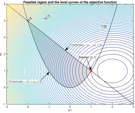
To explain the penalty trajectory intuitively, consider the following example HS7 from the Hock-Schittkowski (HS) test collection. The HS problems are an important subclass of the Constrained and Unconstrained Testing Environment (CUTEst) test collection, which is a commonly used environment for testing optimization algorithms (see Chapter 6 for more details). This example is used repeatedly throughout this chapter.
Example 3.2.1. Consider the following nonlinear equality constrained problem HS7 in two variables. minimize x∈R2 ln(1 +x21)−x2 subject to (1 +x21)2+x22−4 = 0. (HS7)
The unique isolated local (and also global) minimizer of HS7 is x∗ = (0,√3) with unique optimal Lagrange multipliers y∗ = −√3/6, computed from g(x∗) = J(x∗)Ty∗. The level curves of P(x;µ) for a sequence of decreasing µ are shown in Figure 3.1.
(a)µ= 10 (b) µ= 5
(c) µ= 1 (d)µ= 0.1
Figure 3.1: Level Curves of the Conventional Quadratic Penalty Function for Different Values ofµ.
of HS7. It can be observed that asµ→0+, the level curves ofP(x;µ) gradually resemble the
level curves of the constraint function and a sequence of its unconstrained local minimizers approach x∗ vertically from above.
Theorem 3.2.1 provides the main convergence result of the conventional quadratic function method, whose proof can be referred in Fiacco and McCormick [8].
Theorem 3.2.1. Suppose that f(x), c(x) ∈ C2, with y
k = −c(xk)/µk being the penalty multipliers, such that ||∇P(xk;µk)|| ≤ εk where εk → 0 as k → ∞, and that {xk}k≥0
converges to x∗ for which J(x∗) has full rank. Then x∗ satisfies the first-order optimality conditions for (NEP) (see Theorem 2.1.1) and{yk}k≥0 converges to the associated Lagrange
multipliers y∗.
3.2.2
Augmented Lagrangian Method
The augmented Lagrangian method was first proposed by Hestenes [30] and Powell [36], and then developed by Rockafellar [42], Bertsekas [5] and others. Powell derived the augmented Lagrangian method as a shifted penalty function method for which the penalty parameter µdoes not need to converge to zero. The price that has to be paid for keepingµ
bounded away from zero is the need to update the estimated Lagrange multipliers at each iteration. The augmented Lagrangian method is known to be robust in the case where J(x) does not have full rank, i.e., gradient of the constraints are linearly dependent.
The relation of the penalty function method and the augmented Lagrangian method can be understood by considering a problem in which the equality constraint c(x) = 0 is replaced by the shifted constraint c(x)−µyE = 0, i.e.,
minimize x∈Rn
f(x) subject to c(x)−µyE
= 0, (PNEP)
problem (PNEP) is given by b P(x;yE , µ) =f(x) + 1 2µ||c(x)−µy E ||2 =f(x) + 1 2µ ||c(x)|| 2−2µc(x)TyE +µ2||yE||2 .
For a fixed pair (yE, µ), minimizing
b
P(x;yE, µ) is equivalent to minimizing the
aug-mented Lagrangian function defined as
LA(x;y E , µ) = f(x)−c(x)TyE + 1 2µ||c(x)|| 2 .
The main theoretical basis of the conventional augmented Lagrangian method is stated in Theorem 3.2.2, which also indicates thatµy∗ would be the optimal shift, where y∗
is the optimal Lagrange multipliers of (NEP).
Theorem 3.2.2. Supposex∗ satisfies the second-order sufficient conditions for a minimizer of (NEP) (see Theorem 2.1.3). Let y∗ be the corresponding optimal Lagrange multipliers at
x∗. Then there must exist a finite µ >¯ 0, for every 0< µ <µ¯, a solution x∗ of (NEP) is an isolated unconstrained minimizer of LA(x;y
∗, µ).
Proof. By definition, LA(x;y
∗
, µ) =f(x)−c(x)Ty∗+21µ||c(x)||2, the gradient and Hessian of
LA are given by ∇LA(x;y ∗ , µ) = g(x)−J(x)T(y∗− 1 µc(x)) ∇2L A(x;y ∗ , µ) = H(x, y∗ − 1 µc(x)) + 1 µJ(x) TJ(x). (3.8)
The first-order optimality condition implies that if x∗ is a solution of (NEP), then
c(x∗) = 0 and g(x∗)−J(x∗)Ty∗ = 0, which further implies that ∇L
A(x ∗;y∗, µ) = 0 and ∇2L A(x ∗;y∗, µ) = H(x∗, y∗) + 1 µJ(x
∗)TJ(x∗). The second-order sufficient conditions (see
Theorem 2.1.3) imply that the reduced Hessian ZTH(x∗, y∗)Z must be positive definite, where the columns of Z form the basis of null(J(x∗)). According to Debreu’s Lemma (see Lemma 1.4.2), ∇2L
0< µ <µ¯ with some ¯µ >0. Thus x∗ must be an isolated local minimizer of (NEP).
Based on Theorem 3.2.2, Hestenes and Powell proposed thatx∗ be found by minimiz-ing LA(x;y
E
, µ) for a sequence of values of (yE
, µ). For a given pair (yE
, µ),LA(x;y
E
, µ) may be minimized by either a line-search or trust-region method for unconstrained optimization. Once the minimization is complete, (yE, µ) are updated to encourage convergence. Ideally,
the update should allow yE →y∗ in the limit, with µbounded below.
From the proof of Theorem 3.2.2, we know that when minimizing LA(x;y
E, µ), the
associated Newton equation can be expressed by
H(x, π(x)) + 1 µJ(x) TJ(x) p=− g(x)−J(x)Tπ(x). (3.9) A comparison of (3.1) with (3.9) indicates that although they share the “same” structure, the multiplier estimateπ(x) is different, with π(x) =−c(x)/µin the quadratic penalty function method and π(x) = yE −c(x)/µ in the augmented Lagrangian method. The primal-dual
form of the Newton equations (3.9) may be written as
H(x, π(x)) J(x)T J(x) −µIm ∆x −∆y =− g(x)−J(x)Ty c(x) +µ(y−yE) , (3.10) where ∆y = −1 µ(J(x)∆x+ (c(x) +µ(y−y
E))). The diagonal matrix −µI
m in the (2, 2)-block of the KKT matrix serves as a regularization of the KKT system (3.10).
A complete description of the augmented Lagrangian method is given in Algorithm 3.2. The modification of ∇2L
A(xk;yEk, µk) by adding some positive definite Ek is used to guar-antee that pk is a descent direction for LA(x;y
E
, µ). In practice, Ek can be computed “on the fly” while computing the symmetric indefinite factorization of Kµ (See Forsgren and Gill [10]). Given the decreasing sequence {βk}k≥0, if ||c(xk+1)||> βk, then µk is reduced to penalize the constraint violations and enforce feasibility (see Step 13). For efficiency, the multiplier estimate yE is frequently updated in Step 17 if the constraint violations are less
Algorithm 3.2 Augmented Lagrangian Method for (NEP)
1: Choose constants ηs, γc, γ, α, ε with 0< ηs < 12, 0< γc, γ, α <1, and 0< ε1; 2: Choose x0, y0,yE0, µ0 >0, and β0 =α||c(x0)||;
3: Initial iterationk ←0; 4: while not converged do
5: Define positive definite matrixEksuch that∇2LA(xk;ykE, µk)+Ekis positive definite; 6: Solve ∇2L A(xk;y E k, µk) +Ek pk=−∇LA(xk;y E k, µk); . Newton step 7: Set initial step αk ←1;
8: while LA(xk+αkpk;y E k, µk)> LA(xk;y E k, µk) +ηsαk∇LA(xk;y E k, µk)Tpk do
9: αk←γcαk; .Line search along pk
10: end while 11: xk+1 ←xk+αkpk; 12: if ||∇LA(xk+1;y E k, µk)|| ≤εk then 13: if ||c(xk+1)||> βk then
14: µk+1 ←γµk; .Decrease µ to enforce feasibility
15: βk+1 ←α||c(xk+1)||, εk+1 ← 12εk;
16: else
17: yE
k+1 ←y
E
k, µk+1 ←µk; . Update multipliers estimate
18: βk+1 ←βk, εk+1 ←εk;
19: end if
20: end if
21: k ←k+ 1; 22: end while
again. Figure 3.2 shows the level curves of LA(x;y
E, µ) for yE = −0.289, which is the
approximation of the optimal multipliers y∗ =−√3/6, and a decreasing sequence of µ.
(a) yE =−0.289, µ= 10 (b)yE =−0.289, µ= 5
(c)yE =−0.289, µ= 1 (d)yE =−0.289, µ= 0.1
Figure 3.2: Level Curves of augmented Lagrangian Function for Different Values of µ.
In Figure 3.2, the colored level curves of the augmented Lagrangian functionLA(x;y
E, µ) are given for a decreasing sequence of µ. The red elliptic is the feasible region and the blue point represents the solution of HS7. It can be shown that when µ is sufficiently small, then
x∗ is an unconstrained local minimizer of LA(x;y
∗, µ). This implies that x∗ is “contained”
in the center of level curves of LA(x;y
E, µ) and there is no need for reducing µto zero. The
3.3
Motivation of The Proposed Algorithm
This section describes a primal-dual path-following method for (NEP), proposed by Armand et al. [2], which is a Newton-like method applied to a sequence of perturbed opti-mality systems that follow naturally from the quadratic penalty approach. Their algorithm has a “two-level”structure in which the outer iteration involves solving a perturbed KKT linear system and monitoring the residual. If the residual is not sufficiently small, a quadratic penalty function is minimized in the inner iteration to obtain global convergence. It has been shown that whenever the primal-dual pair (xk, yk) converges to a regular solution (x∗, y∗), if µk converges to 0 with a superlinear rate of convergence, then the algorithm reduces asymptotically to Newton iterations and the inner iteration is no longer needed.
The first-order optimality condition for minimizing P2(x;µ) is given by
g(x) + 1
µJ(x)
Tc(x) = 0. (3.11) If y = −c(x)/µ is used as an auxiliary variable, then (3.11) is equivalent to the perturbed optimality condition for (NEP):
F(x, y;µ) = g(x)−J(x)Ty c(x) +µy = 0. (3.12)
Define the primal-dual pairv(µ) = (x(µ), y(µ)), thenF(x, y;µ) = 0 implicitly defines a trajectory µ → v(µ) which passes through the solution (x∗, y∗) as µ → 0. The main idea is to define a sequence of primal-dual iterates (xk, yk) that closely path-follows this trajectory. Specifically, in the outer iteration, the idea is to apply a Newton-like method on F(x, y;µk) = 0 for some decreasing sequence µk > 0. A steadily decreasing sequence of
εk >0 is defined so that if the trial step ||F(x+k, y
+
k;µk)|| ≤εk, then (x+k, y
+
k) is accepted as the next iterate. Otherwise the inner iteration is called where a penalty type merit function that measures the distance of the current iterate to the trajectory is minimized by applying a backtracking line search to obtain global convergence.
The merit function ψµ(v) used in the inner iteration is the primal-dual penalty func-tion proposed by Forsgren and Gill [11]. This funcfunc-tion is the convenfunc-tional quadratic penalty function plus a term that measures the distance of the current iterate to the path-following trajectory. ψµ(v) =f(x) + 1 2µ||c(x)|| 2+ ν 2µ||c(x) +µy|| 2, (3.13)
where ν > 0 is a scaling parameter to balance the penalty of the constraint violations and the distance to the path-following trajectory. v is the primal-dual pair defined as v = (x, y). The gradient and Hessian of ψµ(v) are given by
∇ψµ(v) = g(x) +J(x)T(µ1c(x) + µν(c(x) +µy)) ν(c(x) +µy) ∇2ψ µ(v) = H(x,−(1µc(x) + νµ(c(x) +µy))) νJT νJ νµIm .
It is immediate that every primal-dual pairv = (x, y) on the trajectory defined by the path-following equation (3.12) is a stationary point ofψµ(v). Furthermore, if the second order sufficient conditions of (NEP) (see Theorem 2.1.3) hold at the primal-dual pairv∗ = (x∗, y∗), then ∇2ψ
µ(v∗) must be positive definite, which guarantees that the local minimum could be found.
In a subsequent paper [3], Armand and Omheni extended this method to a primal-dual augmented Lagrangian method for solving the equality constrained minimization problem. This is also a Newton-type method applied to the perturbed optimality conditions but it based on the properties of the augmented Lagrangian function.
The next section describes an alternative perturbed optimality condition that may also be regarded as defining an implicit penalty trajectory. A primal-dual augmented La-grangian merit function is minimized to keep the iterates within a certain neighborhood of the trajectory.
3.4
Description of the Proposed Algorithm
In this section, a detailed description of the proposed primal-dual path-following aug-mented Lagrangian method (PDAL) is given. This method shares a similar “two-level” structure containing both the outer and inner iterations. The idea is to define a trajectory by a perturbed first-order optimality condition and then define a merit function with the potential of giving limit point that satisfies the second-order necessary optimality condi-tions. PDAL is also in part motivated by the Forsgren and Gill primal-dual interior method (See [10]), but is intended to solve only equality constrained problems from a path-following perspective.
In the outer iteration of PDAL, a trial iterate (x+k, yk+) is obtained by applying the modified Newton’s method for finding the approximate solution of F(x, y;yE, µ) = 0, which
is defined by F(x, y;yE , µ) = g(x)−J(x)Ty c(x) +µ(y−yE) , (3.14)
where yE is the current Lagrange multipliers estimate and µ is the penalty parameter. If
(x+k, yk+) reduces ||F(x, y;yE, µ)|| sufficiently, then it is accepted as a new iterate.
Oth-erwise, the inner iteration is called where an augmented Lagrangian type merit function
M(x, y;yEk, µ) defined in (3.17) is minimized to restrict next iterate back to the neighbor-hood of the path-following trajectory.
In fact, the path-following equation (3.14) can be obtained by considering the gra-dient of the conventional augmented Lagrangian function LA(x;y
E, µ) = f(x)−c(x)TyE + 1 2µ||c(x)|| 2, which is given by ∇LA(x;y E , µ) = g(x)−J(x)T yE− 1 µc(x) . If y = yE − c(x)/µ, then ∇LA(x;y E , µ) = 0 is equivalent to F(x, y;yE , µ) = 0, which is exactly (3.14). So the idea is to find zeros of F(x, y;yE, µ) = 0 while updating parametersµ
3.4.1
Description of The Outer Iteration
In the outer iteration of PDAL, a Newton-like method is used for finding the zeros of F(x, y;yE, µ) = 0. At the current iterate (x
k, yk), the linearization of F(x, y;yE, µ) at (xk, yk, µk) with respect to (x, y, µ) is given by:
H(xk, yk) −J(xk)T J(xk) µkIm x+k −xk yk+−yk + 0 yk−yEk (µ + k −µk) =− g(xk)−J(xk)Tyk c(xk) +µk(yk−ykE) ,
whereH(xk, yk) is the Hessian of Lagrangian at (xk, yk), and (x+k, y
+
k) is the next trial iterate. An equivalent butsymmetric linear system can be rewritten as
H(xk, yk) J(xk)T J(xk) −µkIm x+k −xk yk−y+k + 0 yk−yEk (µ + k −µk) = − g(xk)−J(xk)Tyk c(xk) +µk(yk−ykE) .
A simple rearrangement gives
H(xk, yk) J(xk)T J(xk) −µkIm x+k −xk yk−y+k =− g(xk)−J(xk)Tyk c(xk) +µ+k(yk−ykE) . (3.15)
If this KKT matrix is denoted by Kk, then (3.15) can be written as
Kk x+k −xk yk−yk+ =−F(xk, yk;y E , µ+k). (3.16)
Note that the (2,2)-block of Kk is −µkIm while an updated value of µ+k (µ+k < µk) is used on the right-hand side of (3.16).
If the second-order sufficient conditions hold at (x, y) (see Theorem 2.1.3), then the reduced HessianZ(x)TH(x, y)Z(x) must be positive definite. According to Debreu’s Lemma (see Lemma 1.4.2), there must exist a constant ¯µ > 0, such that H(x, y) + µ1J(x)TJ(x) is positive definite whenever 0 < µ < µ¯. The update rule of µk is based on this observation. Specifically, if H(xk, yk) + µ1kJkTJk is not sufficiently positive definite, then the trial µ+k = min µ1+k σ, aµk,1k , whereσ,a∈(0,1). This strategy is the same as the one used by Armand
et al. [2, 3], and it can be observed numerically that as µk →0+, the linear decrease of the formaµk is more acceptable.
Another important issue is that ifKk has more thanmnegative eigenvalues, then the (1,1)-block need to be modified to ensure that In(Kk) = (n, m,0) (and therefore that the reduced Hessian is positive definite). There are many techniques of modifying matrices of the form Kk. One example is to add a positive semidefinite matrix ηkIn to the (1,1)-block of Hk and increase ηk whenever Kk has more than m negative eigenvalues. This technique is applied in Algorithm 3.3. Other techniques include the use of the modified symmetric indefinite factorization of Kk (see, Forsgren, Gill and Murray [14], Gill and Wong [26, 27]).
Once the modified KKT system (3.16) has been solved and the next trial iterate (x+k, yk+) obtained, if ||F(x+k, y+k;yE
k, µ
+
k)||∞ ≤ ρs||F(xk, yk;yEk, µk)||∞ for some 0 < ρs < 1, then (x+k, y+k, µ+k) → (xk+1, yk+1, µk+1) and the Lagrange multiplier estimate is updated by
y+k →yE
k+1. Otherwise the inner iteration is used to reduce ||F(x, y;y
E, µ)||
∞ by minimizing
the merit function using a line-search method.
Note also that the maximum number of inner iteration is limited for efficiency. It is not worthwhile using too many inner iterations to force||F(x+k<