Machine Learning for Hand Gesture Classification from Surface Electromyography Signals

Gesture Classification from

Surface Electromyography Signals

A thesis submitted to the University of Sheffield for the degree of Doctor of Philosophy

Adam Hartwell

Department of Automatic Control and Systems Engineering

Abstract

Classifying hand gestures from Surface Electromyography (sEMG) is a process which has applications in human-machine interaction, rehabilitation and pros-thetic control. Reduction in the cost and increase in the availability of necessary hardware over recent years has made sEMG a more viable solution for hand ges-ture classification. The research challenge is the development of processes to ro-bustly and accurately predict the current gesture based on incoming sEMG data.

This thesis presents a set of methods, techniques and designs that improve upon evaluation of, and performance on, the classification problem as a whole. These are brought together to set a new baseline for the potential classification.

Evaluation is improved by careful choice of metrics and design of cross-validation techniques that account for data bias caused by common experimental techniques. A landmark study is re-evaluated with these improved techniques, and it is shown that data augmentation can be used to significantly improve upon the performance using conventional classification methods.

A novel neural network architecture and supporting improvements are pre-sented that further improve performance and is refined such that the network can achieve similar performance with many fewer parameters than competing designs. Supporting techniques such as subject adaptation and smoothing algorithms are then explored to improve overall performance and also provide more nuanced trade-offs with various aspects of performance, such as incurred latency and pre-diction smoothness.

A new study is presented which compares the performance potential of med-ical grade electrodes and a low-cost commercial alternative showing that for a modest-sized gesture set, they can compete. The data is also used to explore data labelling in experimental design and to evaluate the numerous aspects of perfor-mance that must be traded off.

ii

Acknowledgements

I’d first like to express my thanks to my supervisor Dr. Sean Anderson. His guid-ance has been invaluable in improving not just my research but also improving my own skill set, particularly with regards to writing. His enthusiasm was critical for helping me achieve this culmination of my work and helped motivate me during times where I struggled.

I also want to thank my second supervisor Professor Visakan Kadirkamanathan for his useful advice, suggestions and insight on the varied topics and problems I’ve consulted with him about. I’d also like to thank him for cajoling me into tak-ing a more active part in our research community and givtak-ing me the opportunity to do so.

I would like to thank my partner Dawn for her love and support and always knowing how to put a smile on my face when I needed it.

I’d like to thank the numerous other researchers and colleagues who gave me the opportunity to discuss interesting problems and gave me new insight or perspective. I’m also thankful for the opportunities given to me by same to teach and present which have been both fulfilling and a perfect opportunity to solidify my own knowledge base.

My friends, I thank for keeping me sane and reminding me to keep things in balance.

Lastly, I’d like to thank my parents Stephen and Ewa for their love, patience and understanding as well as their support, willingness to debate me on my ideas and instilling in me a desire to learn.

Abbreviations xi

Nomenclature xiv

1 Introduction 1

1.1 Background . . . 1

1.2 Aims and Objectives . . . 3

1.3 Thesis Structure . . . 4 1.4 Associated Publications . . . 5 2 Literature Review 7 2.1 Electromyography . . . 7 2.1.1 Biological Basis . . . 7 2.1.2 Characteristics of sEMG . . . 9

2.1.3 Signal Processing Issues . . . 9

2.1.4 Summarised History of EMG . . . 10

2.1.5 Electrode Types . . . 10

2.1.6 Skin Preparation and Electrode Placement . . . 11

2.1.7 Applications of sEMG . . . 12

2.1.8 Myo Armband . . . 13

2.2 Machine Learning Overview . . . 14

2.2.1 Feature Engineering . . . 14

2.3 Neural Networks and Deep Learning . . . 15

2.3.1 No Free Lunch Theorems . . . 16

2.3.2 The Neuron Model . . . 16

2.3.3 Training and Backpropagation . . . 17

2.3.4 Activation Functions . . . 23

2.3.5 Network Architectural Choices . . . 28

2.4 Hand Movement Classification . . . 34

2.4.1 Deep Learning Approaches . . . 37 iii

iv Contents

2.4.2 Key Issues . . . 38

3 Methods 40 3.1 Statistics for Comparison of Techniques . . . 40

3.1.1 Comparison of Two Techniques . . . 41

3.1.2 Comparison of Multiple Techniques . . . 41

3.2 Machine Learning Algorithms . . . 43

3.2.1 Support Vector Machines . . . 43

3.2.2 K Nearest Neighbours . . . 46

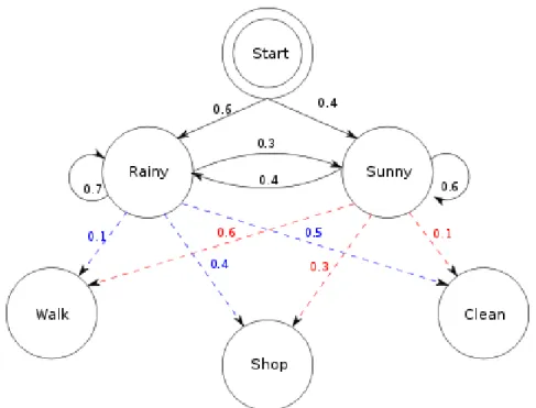
3.2.3 Hidden Markov Models . . . 46

3.3 Evaluation Metrics . . . 49

3.3.1 Binary Case . . . 49

3.3.2 Multiclass Case . . . 50

3.4 Data Labelling . . . 52

4 Robust Feature-Based Classification 55 4.1 Introduction . . . 55

4.2 Data Analysis . . . 57

4.3 Robust Preprocessing and Evaluation . . . 61

4.3.1 Windowing . . . 61 4.3.2 Metrics . . . 65 4.3.3 Validation . . . 67 4.4 Benchmark Details . . . 69 4.4.1 Preprocessing . . . 69 4.4.2 Features . . . 70 4.4.3 Classifiers . . . 71

4.4.4 Validation and Metrics . . . 72

4.4.5 Meta-Validation . . . 73

4.4.6 Data Resampling and Augmentation Techniques . . . 74

4.4.7 Primary Benchmark Variants . . . 75

4.4.8 Person-specific Movement Set Selection . . . 76

4.5 Results and Discussion . . . 79

4.5.1 Benchmark Results . . . 79

4.5.2 Metric Comparison . . . 79

4.5.3 Benchmark Performance Breakdown . . . 81

4.5.4 Feature Differences . . . 84

4.5.5 Comparison of Window Lengths . . . 86

4.5.6 Classifier Trends . . . 87

4.5.8 Movement Sub-selection Results . . . 90

4.6 Conclusion . . . 93

5 Deep Neural Networks for Person-Specific Classification 94 5.1 Introduction . . . 94

5.2 Methodology . . . 95

5.2.1 Baseline SVM-RBF . . . 97

5.2.2 Baseline CNN . . . 99

5.2.3 Temporal-to-Spatial Network . . . 101

5.2.4 Additional Design Choices . . . 103

5.2.5 Adam Algorithm . . . 105

5.2.6 Comparison to Contemporary Networks . . . 106

5.2.7 Filter Visualisation . . . 107

5.3 Results and Discussion . . . 108

5.3.1 Effect of Repetition Number . . . 110

5.3.2 Distribution of Classification Performance . . . 111

5.3.3 Filter Visualisations . . . 112

5.4 Conclusion . . . 113

6 Compact Deep Neural Networks with Comparison of Electrodes 119 6.1 Introduction . . . 119 6.2 Methods . . . 120 6.2.1 Experiment Overview . . . 120 6.2.2 Experiment Protocols . . . 122 6.2.3 Experiment Software . . . 126 6.2.4 Experiment Extensions . . . 127 6.2.5 Electrode Comparison . . . 127 6.2.6 Data Preprocessing . . . 128 6.2.7 Performance Baselines . . . 129

6.2.8 Compact Deep Neural Network . . . 130

6.2.9 Hardware Performance Comparison . . . 131

6.3 Results and Discussion . . . 132

6.3.1 Key Findings . . . 132

6.3.2 Performance on Hardware . . . 135

6.3.3 GLR vs Hold vs Expert Labelling . . . 136

vi Contents

7 Online Classification 141

7.1 Introduction . . . 141

7.2 Methods . . . 142

7.2.1 Improving Performance with Transfer Learning . . . 142

7.2.2 Motivation for Smoothing Predictions . . . 145

7.2.3 Latch Algorithm . . . 148

7.2.4 Majority Voting Algorithm . . . 148

7.2.5 The MSPRT Algorithm . . . 149

7.2.6 Smoothing with Hidden Markov Models . . . 149

7.2.7 Viterbi Algorithm . . . 150

7.3 Results and Discussion . . . 151

7.3.1 Subject Adaptation . . . 151

7.3.2 Prediction Smoothing . . . 153

7.4 Integration of Techniques . . . 159

7.5 Conclusion . . . 160

8 Closing Remarks 163 8.1 Summary and Conclusions . . . 163

8.2 Future Research Avenues . . . 165

2.1 Illustration of the formation of an EMG signal . . . 8

2.2 Ideal Bipolar Electrode Placement . . . 12

2.3 The Myo Armband . . . 13

2.4 Biological Neuron and Neural Network Neuron . . . 17

2.5 Visualisation of Chain Rule . . . 19

2.6 Comparison of Momentum and Nesterov Momentum . . . 21

2.7 Dropout Layer Visualisation . . . 24

2.8 Logistic Sigmoid Activation . . . 25

2.9 Tanh Activation . . . 26

2.10 Rectified Linear Unit Activation . . . 27

2.11 Basic Neural Network . . . 28

2.12 Visualisation of Convolutional Layer . . . 31

2.13 Visualisation of Stride . . . 32

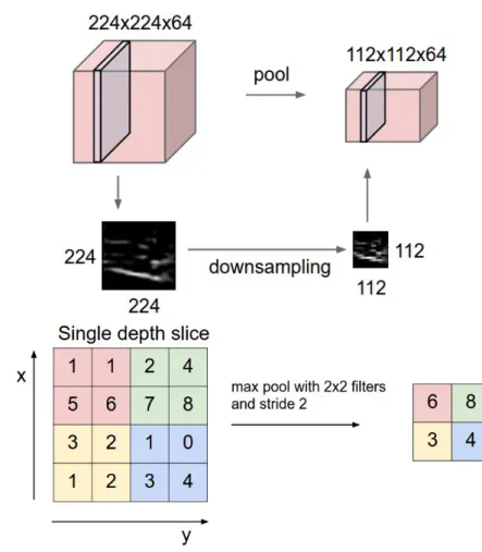
2.14 Pooling Layer Visualisation . . . 34

2.15 LSTM and GRU Visualisation . . . 35

3.1 SVM Mapping and Decision Boundary . . . 45

3.2 HMM Visualisation as Bayesian Network . . . 47

3.3 Hidden Markov Model . . . 48

4.1 Illustration of Data Imbalance . . . 59

4.2 PCA Visualisation . . . 60

4.3 t-SNE Visualisations . . . 62

4.4 Windowing Visualisation . . . 63

4.5 Visualisation of Windowed sEMG . . . 64

4.6 Histogram of Accuracies from NinaPro Study . . . 66

4.7 Example Comparison of Metrics . . . 83

4.8 Gesture Sub-selection Comparison . . . 91

5.1 Visualisation ofXω . . . 98

viii List of Figures

5.2 TtS Network Diagram . . . 101

5.3 Geng et al. Performance Per Class . . . 109

5.4 TtS Performance by Repetition Number . . . 115

5.5 Normalised Position in Movement Against Performance, NinaPro Study . . . 116

5.6 Normalised Position in Movement Against Performance . . . 116

5.7 Visualisation of Temporal Convolution Weights . . . 117

5.8 Visualisation of Temporal Convolution Maximum Activation Inputs 117 5.9 Visualisation of Spatial Reduction Maximum Activation Inputs . . . 118

6.1 Jetson TX2 . . . 120

6.2 Electrode Positioning . . . 123

6.3 Set of Gestures . . . 123

6.4 Normalised Position in Movement Against Performance . . . 126

6.5 Myo v Delsys Per Class Performance . . . 133

6.6 Myo v Delsys Per Subject Performance . . . 133

6.7 Myo v Delsys Performance Subject 1 . . . 134

6.8 Myo v Delsys Performance Subject 2 . . . 135

6.9 Comparison of Gesture Labelling Methods . . . 138

7.1 Classification Flicker . . . 145

7.2 Latency Definitions . . . 146

7.3 Pareto Frontier of Smoothing Algorithms (Onset) . . . 158

7.4 Pareto Frontier of Smoothing Algorithms (Tail) . . . 159

3.1 Binary Confusion Matrix . . . 49

3.2 Multiclass Confusion Matrix . . . 51

4.1 Table of Features . . . 70

4.2 Benchmark Training and Test Repetitions . . . 72

4.3 100ms Benchmark Results . . . 80

4.4 200ms Benchmark Results . . . 81

4.5 400ms Benchmark Results . . . 82

4.6 Average Rank Against Set Size . . . 92

5.1 Training and Test Sets . . . 96

5.2 Baseline CNN DB1 . . . 99 5.3 Baseline CNN DB2 . . . 99 5.4 Baseline Adapted CNN DB2 . . . 99 5.5 TtS DB1 . . . 102 5.6 TtS DB2 . . . 102 5.7 Adapted TtS DB2 . . . 102

5.8 Deep Learning Results Database 1 . . . 108

5.9 Deep Learning Results Database 2 . . . 108

6.1 Study Training, Validation and Test Repetitions . . . 129

6.2 Compact TtS (Myo Data) . . . 131

6.3 Compact TtS (Delsys Data) . . . 131

6.4 Network Performances and Run Time on Jetson TX2 . . . 136

6.5 Comparison of Labelling Techniques . . . 137

7.1 Updated TtS . . . 143

7.2 Study Training, Validation and Test Repetitions . . . 143

7.3 Subject Adaptation Results . . . 151 7.4 Subject Adaptation Results When Trained On Individual Repetitions 152

x List of Tables

7.5 Supplemental Smoothing Results (Expert Trained, Expert Tested) . . 154 7.6 Supplemental Smoothing Results (GLR Trained, Expert Tested) . . . 154 7.7 Supplemental Smoothing Results (Expert Trained, GLR Tested) . . . 155 7.8 Supplemental Smoothing Results (GLR Trained, GLR Tested) . . . . 155 7.9 Cross-Validated Smoothing Results . . . 157

ANOVA Analysis Of Variance. 42

API Applications Programming Interface. 14 AUC Area Under Curve. 50

CNN Convolutional Neural Network. 30, 32, 33, 99, 113 DSP Digital Signal Processing. 61

DT Decision Tree. 71, 87, 88

DWT Discrete Wavelet Transform. 70 ECG Electrocardiography. 7, 10 ECoG Electrocorticography. 1, 2 EEG Electroencephalography. 1, 103 EM Expectation Maximisation. 149 EMG Electromyography. 1, 7, 9, 10, 14, 23, 34, 36, 37, 53, 58, 61, 63, 65, 67, 68, 69, 70, 76, 101, 156, 166

FFT Fast Fourier Transform. 37 FN False Negative. 49, 50, 51, 65 FP False Positive. 49, 50, 51, 65

GLR Generalised Likelihood Ratio. 53, 57, 61, 120, 125, 127, 137, 138, 139, 140, 147, 153, 154, 155, 156, 157, 159

GPU Graphics Processing Unit. 18, 96, 107, 120 xi

xii Abbreviations

GRU Gated Recurrent Unit. 34, 35 HIST Histogram. 70, 84, 85, 86

HMM Hidden Markov Model. 46, 47, 48, 149, 150, 158 IMU Inertial Measurement Unit. 14

JSON Javascript Object Notation. 124 KL Kullback-Leibler. 78, 92

KNN K-Nearest Neighbours. 46, 71, 87, 88

L-BFGS Limited-Memory Broyden-Fletcher-Goldfarb-Shanno. 22 LDA Linear Discriminant Analysis. 36, 71, 84, 85, 87, 88

LSTM Long Short-Term Memory. 34, 35, 104 MAE Mean Absolute Error. 19, 20, 74, 89, 90

MAV Mean Absolute Value. 70, 77, 85, 86, 88, 92, 98, 103, 112, 113

mDWT Mariginal Discrete Wavelet Transform. 70, 73, 74, 77, 83, 84, 85, 86, 88, 89, 98, 112, 129

ML Machine Learning. 16

MLP Multilayer Perceptron. 16, 28, 71 MSE Mean Squared Error. 19, 20

MSPRT Multi-Hypothesis Sequential Probability Ratio Test. 149, 157, 158

NinaPro Non-Invasive Adaptive Hand Prosthetics. 35, 36, 37, 38, 57, 65, 66, 95, 106, 111, 125, 131, 156

PCA Principal Component Analysis. 59, 61 RBF Radial Basis Function. 46

ReLU Rectified Linear Unit. 26, 27, 28 RF Random Forest. 36

RMS Root Mean Squared. 57, 69

ROC Receiver Operating Characteristic. 50, 52

sEMG Surface Electromyography. i, 1, 2, 3, 4, 7, 8, 9, 10, 11, 12, 13, 14, 15, 35, 36, 37, 43, 52, 55, 57, 64, 89, 93, 94, 98, 99, 100, 103, 104, 106, 112, 137, 139, 140, 141, 145, 151, 159, 160, 162, 163, 164, 165, 166

SGD Stochastic Gradient Descent. 20, 21

SMOTE Synthetic Minority Oversampling Technique. 74, 75, 81, 82, 83, 84, 85, 89, 100, 132, 159, 160

SVM Support Vector Machine. vii, 36, 42, 43, 44, 113, 116 SVM-L Support Vector Machine - Linear Kernel. 71, 87, 88

SVM-RBF Support Vector Machine - Radial Basis Function Kernel. 45, 71, 73, 74, 83, 87, 88, 89, 97, 98, 108, 129, 132

t-SNE t-Stochastic Neighbour Embedding. 61, 107 TN True Negative. 49, 50, 51, 65 TP True Positive. 49, 50, 51, 65 TtS Temporal-to-Spatial. 101, 102, 108, 109, 110, 111, 112, 113, 115, 116, 117, 118, 119, 120, 126, 129, 130, 131, 132, 133, 134, 135, 136, 137, 139, 140, 143, 144, 159, 160, 161 VAR Variance. 70, 85, 86 WL Waveform Length. 70, 85, 86, 98

Nomenclature

A list of the variables and notation used in this thesis is defined below. The def-initions and conventions set here will be observed throughout unless otherwise stated.

[a,b] Closed interval betweenaandb

ˆ

x Estimate ofx

∈ Member of operator

∨ Logical "OR" operator

RD _{Real numbers of dimensionsD}

L Loss µ Mean σ Standard deviation b Bias term P(A) Probability of event A w Weight term

X A set of data points

x A data point

Y A set of outputs

y An output

Introduction

1.1

Background

Surface Electromyography (sEMG) records electrical signals from changes in mus-cle membrane potential with non-invasive electrodes placed on the skin [1]. These signals have applications in prosthetic control [2, 3], rehabilitation [4] and as a natural control interface for human-machine interaction [5]. Hand gesture classifi-cation plays an important role in both human-machine interaction and prosthetic control as a way of determining user intention. Therefore the accurate classifica-tion of hand gestures is a vital step towards realising these applicaclassifica-tions.

This work focuses on framing and solving the hand gesture classification prob-lem with an emphasis on practical considerations. The classification probprob-lem is tackled by improving upon current data preparation and evaluation methods, ap-plying novel deep learning methods, exploring methods for subject adaptation and gathering data to support hardware choices.

Gesture-based interaction or control has applications in many areas. This includes entertainment via games consoles such as the Wii [6], Kinect [7] and PlayStation Move [6], control of dashboard utilities in cars [8, 9], operating surgi-cal equipment [10], aiding in rehabilitation [11] and augmenting working environ-ments [12] amongst others.

Electroencephalography (EEG) and Electrocorticography (ECoG) are alterna-tive methods of extracting user intention from the brain directly via electrodes. These methods, however, are not currently practical for routine clinical or per-sonal use [13]. When using EEG or ECoG user intention needs to be extracted from among a multitude of other signals [14]. Meanwhile, Electromyography (EMG) allows focussing on specific groups of muscles as they are manipulated via the nervous system, which improves intention extraction relative to EEG and

2 1.1. Background

ECoG [13].

An alternate way of recognising gestures is by using a camera which has the benefit of being generalisable to tracking any part of the human body but can require markers to be worn for precise tracking [15]. Camera-based approaches suffer from occlusion problems and may be sensitive to environmental issues such as changes in lighting, obstructions or varying distance from the camera. Gloves with flex sensors have also been trialled [16] which alleviate many of the environ-mental issues of cameras but require substantial hardware adjustment for different users. These two approaches cannot be used with amputees.

In general, the major benefits of sEMG over other methods is that it is not inva-sive, adaptation to individuals can generally be performed in software, it does not suffer from normal changes in the environment, and it can be used on amputees. Having access to user intention via muscle contraction also allows remapping of muscle contraction and intention for prosthetic control [17], which makes sEMG a versatile data source.

This thesis focuses on the problem of classifying hand gestures from sEMG with a general view towards application as a human-machine interface but presents ideas relevant to any application. It aims to improve the overall performance of gesture classification in as generalisable way as possible.

Studies on hand gesture classification with sEMG generally focus on smaller sets of movements, e.g. 4-7 [18–28] or 9-12 movements [29–35]. Most studies, e.g. [20, 23, 27, 30, 34–40], by necessity, employ rest-movement-rest cycles as part of their experiment design and label their data as such which often causes significant data imbalance. Typically accuracy is then used to evaluate these experiments [25, 27, 37, 41–43] or "accuracy" / "classification accuracy" is stated without an equation [18, 20, 23, 26, 28, 29, 35, 37–40, 44, 45] which can lead to uncorrected bias in results.

The key challenges are the design of standard robust evaluation methods for ensuring representative performance reporting and comparability between stud-ies, improving the overall performance of classification techniques, tailoring so-lutions to individual subjects and addressing issues that arise when classifying online.

Therefore the first issue tackled is the improvements that can be made to eval-uation methods. It is shown that common experiment design paradigms lead to biased data sets and thus biased results. The macro-average accuracy is presented as a viable alternative metric that avoids the skew the typical accuracy metric in-troduces. It is combined with proper cross-validation (a technique that is missing in many studies [22–25, 30, 37, 39, 46–49]) and a new stratification technique that

produces a result more representative of the performance that would be found when evaluating all possible folds.

These evaluation techniques are then applied to a reproduction of a landmark open-data study with many hand gestures [37], 52, rather than the typical ≤ 12, to demonstrate the technique’s necessity and that effective classification can be achieved with this higher number of gestures. The study is further improved upon via data augmentation techniques which allow a new performance baseline to be established.

In order to further improve overall performance, a novel neural network ar-chitecture is then designed. It is shown that this arar-chitecture outperforms both the baseline and other neural network approaches to the problem [39, 47]. The network architecture is later refined such that it can produce a similarly high per-formance as the original while requiring an order of magnitude fewer parameters. The new compact design is evaluated on an embedded system, the Jetson TX2, to demonstrate the run time improvement it produces.

Supporting methods including gesture subselection, subject adaptation, and post-classification smoothing are explored as other viable ways to improve perfor-mance and to show the large decision space associated with defining perforperfor-mance outside of only an accuracy measure.

These techniques together present a reliable, robust way of improving overall classification performance and allowing researchers to make informed decisions regarding the trade-offs involved for any particular application. A new study is also presented that compares medical grade electrodes with a low-cost commercial alternative illustrating that the techniques can be used achieve similar performance levels with both helping to make the necessary hardware for classification more accessible.

1.2

Aims and Objectives

This thesis aims to improve sEMG-based gesture classification. Accordingly, the objectives are as follows:

• Reproduce and benchmark existing approaches for gesture classification us-ing conventional classifiers. Improve evaluation and cross-validation to lay the groundwork for robust benchmarking in this thesis and future studies • Investigate how the number of gestures classified affects performance to

es-tablish a realistic number of gestures on which high performance can be achieved and evaluate algorithms for person-specific gesture subselection

4 1.3. Thesis Structure

• Reproduce, benchmark and extend the design of the current state of the art in deep neural networks for EMG-based gesture classification using state of the art techniques along with robust evaluation and validation

• Extend the current state of the art by designing novel deep neural networks suited to embedded systems that exploit compression techniques and do-main knowledge

• Compare new generation low-cost consumer surface EMG electrodes to ex-pensive medical grade electrodes to establish the viability of low-cost elec-trodes

• Extend the state-of-the-art in online EMG classification by augmenting deep neural network classifiers with smoothing methods to prevent class ’jitter’ within the classification signal

1.3

Thesis Structure

This thesis is structured around the central idea of improving sEMG gesture clas-sification:

• Chapters 2 and 3 introduce the theories, techniques, and background this work is built upon. Particular attention is given to machine learning tech-niques and neural networks. These chapters are intended as a reference that supports the later chapters.

• Chapter 4 proposes a set of fundamental improvements to the classification process that are necessary to ensure that results are reproducible and repre-sentative. A landmark study is repeated and shown to have significantly bi-ased results, data resampling and augmentation methods are then applied to significantly improve performance over the original. Lastly, a novel evalua-tion of gesture sub-selecevalua-tion techniques is presented, which demonstrates the possibility for further performance improvement via patient-specific adapta-tion outside of the classifiers themselves.

• Chapter 5 introduces a novel neural network architecture that encodes do-main knowledge into its design, leading it to significantly outperform con-temporary designs. The network is evaluated across two data sets and against the top performing contemporary designs to demonstrate its im-provement.

• Chapter 6 introduces a new study that compares high- and low-cost elec-trodes finding that the low-cost elecelec-trodes have the potential to produce a similar or better performance on at least some variants of the classification problem. A new compact version of the network design is also introduced that greatly reduces the number of parameters necessary for similar levels of classification performance. The new study’s data is then used to evaluate the run time impact of the parameter reduction, demonstrating real-world run time reduction, which is vital for actual usage. Lastly, different labelling methods are explored to improve upon future experiment designs.

• Chapter 7 explores subject adaptation and online classification signal smooth-ing in order to further improve resultant classification performance. Subject adaptation results show that it is possible to fine-tune a network trained on other subjects to a new individual by freezing the feature extractor layers in a way that improves performance over training directly on a new subject. A variety of techniques are explored for signal smoothing, and it is shown that most lie on the Pareto frontier between smoothness and added latency, although different techniques have additional benefits and drawbacks. • Chapter 8 concludes the thesis. The development of improved classification

methods and techniques is summarised, and potential future avenues for research are presented.

1.4

Associated Publications

The following papers have resulted from work on this PhD:

• Person-Specific Gesture Set Selection for Optimised Movement Classification from EMG Signals

- A. Hartwell, V. Kadirkamanathan, and S.R. Anderson. Person-Specific Ges-ture Set Selection for Optimised Movement Classification from EMG Signals. InProceedings of the 38th Annual International Conference of the IEEE Engineer-ing in Medicine and Biology Society, pages 880–883, 2016

• Compact Deep Neural Networks for Computationally Efficient Gesture Clas-sification From Electromyography Signals

- A. Hartwell, V. Kadirkamanathan, and S.R. Anderson. Compact Deep Neu-ral Networks for Computationally Efficient Gesture Classification From Elec-tromyography Signals. InProceedings of the 7th IEEE RAS/EMBS International Conference on Biomedical Robotics and Biomechatronics, pages 891–896, 2018

6 1.4. Associated Publications

Further papers are under review and being prepared for publication at the time of submission.

The set of tools and utilities developed for this work will be made freely avail-able on GitHub [52], and specific libraries are availavail-able via Python’s package man-ager. The associated scripts and data will be available alongside this thesis via the University of Sheffield’s White Rose system.

The following papers resulted from collaborations with fellow researchers: • Multi-Compartmentalisation in the MAPK Signalling Pathway Contributes

to the Emergence of Oscillatory Behaviour and to Ultrasensitivity

- A. Shuaib, A. Hartwell, E. Kiss-Toth, and M. Holcombe. Multi-Compartmentalisation in the MAPK Signalling Pathway Contributes to the Emergence of

Oscilla-tory Behaviour and to Ultrasensitivity. PLOS ONE, 11(5):e0156139, 2016 • Top-Down Bottom-Up Visual Saliency for Mobile Robots Using Deep Neural

Networks and Task-Independent Feature Maps

- U. Jaramillo-Avila, A. Hartwell, and S. Anderson. Top-Down Bottom-Up Visual Saliency for Mobile Robots Using Deep Neural Networks and Task-Independent Feature Maps. In Proceedings of the 19th Annual Conference: To-wards Autonomous Robotic Systems, volume 10965, page 489. 2018

Literature Review

This chapter covers the necessary background information and relevant literature used to inform later chapters. The key topics covered here are the basis and char-acteristics of Electromyography (EMG) signals, the machine learning techniques used in this work along with a particular focus on modern neural networks and the current academic landscape of EMG based interaction and control.

2.1

Electromyography

2.1.1 Biological Basis

Electromyography (EMG) is the recording of electrical activity produced by mus-cle fibres when they contract [55]. Musmus-cles themselves are formed of bundles of muscle fibres which are a form of long tubular cell. The EMG signal is made up of a superposition of the signals from each muscle cell modified by a person’s physiology.

In a biomedical context, the recorded EMG waveform is known as an elec-tromyogram and is closely related to other bioelectrical signals such as Electrocar-diography (ECG). ECG deals specifically with the signals from heart muscles.

The electrical source for the readings is the change in muscle membrane poten-tial which causes muscle contraction and the associated movement of potassium and calcium ions [1]. Therefore a useful interpretation of the resultant electrical activity is an indirect measurement of movement intention modified by the local physiological and anatomical properties of a subject at the location(s) of interest. The reading is sometimes referred to as the myoelectric signal.

There are two main methods of acquisition for EMG signals: invasive (also referred to as intramuscular) and non-invasive. The non-invasive method is the focus of this thesis and is often referred to as Surface Electromyography (sEMG).

8 2.1. Electromyography

The non-invasive method is also the generally preferred method where possible since it is relatively free of discomfort and presents a much lower risk of infection [56, 57].

Acquisition of sEMG is generally achieved by placing electrodes on the surface of the skin to record the electrical activity. This is in contrast to invasive methods which require placement of electrodes under the skin. Invasive methods allow placement of electrodes closer to specific muscles of interest but are less practical for general usage. Invasive methods have also been shown to produce higher inter-subject variability as well a lower repeatability over extended periods of time [58].

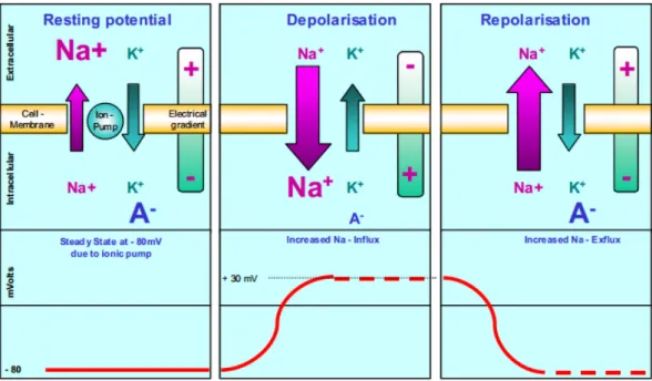
An illustration of the EMG signal in relation to a muscle cell membrane po-tential change is shown in figure 2.1. The figure shows a rough approximation of how the movement of Sodium and Potassium ions across cell membranes (via active transport) produces the observed electrical potential changes as might be viewed by an electrode.

Figure 2.1: Illustration of how an EMG signal is formed by the depolarization and repolar-ization of the muscle membrane in skeletal muscles. The model is simplified to highlight the important phases [59].

The resting potential of the muscle fibre membrane is ∼-80/-90mV [1, 59] rel-ative to the outside of the cell when not contracted. This difference is maintained by ion pumps, as shown in Figure 2.1, which provide the active transport. Then when alpha-motor anterior horn cell is activated either by reflex or via the central nervous system, the excitation is conducted along the motor nerve leading to an

electrical potential being formed at the motor endplates. This causes the diffusion characteristics of the muscle fibre membrane to change, leading to sodium ion in-flow. The membrane, therefore, becomes depolarized, which is quickly reversed via the ion pumps leading to repolarization [59].

2.1.2 Characteristics of sEMG

Figure 2.1 presents a simplified view of the EMG signal itself, which is also more complicated in practice. The key characteristics of sEMG signals are:

• Amplitudes in theµVto lowmVrange depending on muscle type and

con-dition [60, 61]

• The resting potential is typically∼-80/-90mV [1, 59]

• Two distinct phases: transient followed by a steady state[62]

– During contraction, voltages may be either positive or negative [55] • Bandwidth for most significant activity in the range 5-500Hz although other

bandwidths such as 20-450Hz are used depending on area and application of interest [59, 63–65]

– The entire usable range is 0-500Hz [66, 67] – The most significant spectrum is 50-150Hz [66]

• May be modelled as a non-stationary stochastic process [55, 66]

• Composite of all the muscle fibre potentials underneath or near each elec-trode [55]

2.1.3 Signal Processing Issues

From a signal processing standpoint, the major issues that must be considered are: • Motion artefacts caused by movement of electrode relative to the skin

(typi-cally 0-20Hz) [55, 66]

• Quasi-randomness of motor unit firing [55, 66]

• Electrode design (particularly self-interference from circuitry design) [37, 55, 66]

• Electrode placement determines which muscle fibres will be targeted and precise anatomy varies significantly between individuals [68]

10 2.1. Electromyography

• Cross-talk from nearby muscles [56]

• Muscle fatigue alters the action potentials of muscles [68, 69]

• Interference from Electrocardiography (ECG) signals [59] (when near the heart)

• Interference from nearby equipment or power supplies (generally 50-60Hz)

2.1.4 Summarised History of EMG

The term EMG was first used by French scientist Étienne-Jules Mare in 1890 how-ever work on what would now be called EMG is recorded as far back as 1666 when experiments were performed on the muscles of electric ray fish[70]. The beginnings of clinical usage began in 1922 when it was shown that the electrical signals from muscles could be recorded and analysed [71]. The first use of sEMG was in 1966 to monitor the activity of speech muscles [72]. This work was ex-panded upon in 1983 when a clinical method was introduced that demonstrated sEMG could be used to assess the neuromuscular contribution to pain states [73]. Since 1983 EMG and sEMG have mostly been used in clinical and research settings. Primary uses include robot control [74], identification of neuromuscular disorders [75], rehabilitation [76] and prosthetic control [77].

In late 2014 Thalmic Labs shipped an sEMG device called the Myo Armband [78] which provided a low cost, user-friendly way of gathering and using sEMG data in real time. The low cost of the device means that the electrode (and thus signal) quality is not comparable to medically certified devices. The commerciali-sation of an sEMG device, however, moved sEMG toward wider spread usage.

2.1.5 Electrode Types

Invasive EMG (intramuscular) data acquisition typically makes use of needle elec-trodes that use a pointed tip as a detection surface or fine wire elecelec-trodes that utilise small diameter wires typically made of a non-oxidising alloy [79]. Applica-tion of these kinds of electrodes often requires strict certificaApplica-tion and supervision to ensure no harm is done to the subject.

There are two types of electrode typically used when gathering sEMG data: Gelled electrodes and Dry electrodes [80].

Gelled electrodes use an electrolytic gel as an interface between skin and elec-trode, which acts to minimise electrical noise. In this setup, a redox reaction occurs at the metal junction of the electrodes producing the observed signal.

Gelled electrodes are also manufactured in single-use and reusable variants with the single-use variant being most common. The main drawback of gelled electrodes is the greater need for special skin preparation, such as hair removal and cleaning as well as the need to apply the gel to the subject, which can make usage cumbersome.

Dry electrodes forgo the gel interface and place the metal contact directly on the skin. These electrodes often contain multiple detecting surfaces and integrated pre-amplification/filtering circuitry to improve signal quality. Due to the desir-ability of local circuitry, dry electrodes are usually heavier than a gel counterpart. This added weight can lead to issues with keeping the electrodes affixed to the subject and in a stable relationship with the muscles. Engineering for platform stability is, therefore, seen as vital.

Furthermore, sEMG sensors may be classified as active or passive. Passive elec-trodes do not use any filtering/amplification circuitry prior to signal output while active sensors do; therefore, most dry electrodes fall under the active category.

The most common material for the metallic contact of electrodes is silver-silver chloride (Ag-AgCl) which in 2002 was estimated to be used in 80% of sEMG applications [80]. Ag-AgCl is popular because of its relatively low impedance and low half-cell potential [81]. It is considered "the gold standard" material for sEMG electrodes at the time of writing [82].

In general intramuscular electrodes provide better quality and better-targeted recordings since they can be placed closer to specific muscles (including muscles deeper within the body) thus reducing cross-talk and improving discrimination. However, for human-machine interaction purposes, it is highly undesirable to re-quire invasive procedures; therefore, surface electrodes are much better suited to the task.

2.1.6 Skin Preparation and Electrode Placement

Proper skin preparation improves the quality of the sEMG signal received when using any type of surface electrode. Specifically, skin preparation aims to provide impedance matching between skin and electrode. This maximises power transfer between the two by minimising signal reflection. Ideally, all hair and other dead skin cells, as well as moisture, would be removed from the electrode locations. The typical advice is to use an abrasive gel to reduce the dry layer of skin and then clean with alcohol to eliminate moisture [79].

Most surface electrodes utilise two detecting surfaces in a bipolar configura-tion. In this configuration, the detecting surfaces should be 1−2cm apart [66]. The ideal placement for this kind of electrode involves adjusting the electrode’s

longi-12 2.1. Electromyography

tudinal axis (that which intersects both detection surfaces) parallel to the length of the muscle fibres. The electrode should also be between the motor unit and tendon insertion of the muscle of interest, empirically placing detection surfaces on the belly of the muscle has proven to produce good results; likely due to this being the location of highest muscle fibre density [66]. Figure 2.2 shows this ideal placement; as can be seen in the figure this placement maximises intersection with muscle fibres, which results in an improved signal due to the electrical superposi-tion of the resultant signals.

Figure 2.2: Ideal positioning for a bipolar electrode maximising intersection with muscle fibres [66].

2.1.7 Applications of sEMG

Key sEMG applications are:

Human-Computer Interaction, which has the potential to provide a more nat-ural interface for controlling computers and devices. For users with a physical disability, sEMG also has the potential to improve the interaction experience con-siderably.

Physiotherapy and Rehabilitation, typically an electromyogram can be recorded to evaluate the activity of skeletal muscles that a doctor may analyse to determine whether a patient’s muscles are working correctly. Beyond this basic human-in-the-loop use, however, research is being conducted to automate this detection [83] and provide feedback not just to doctors making an assessment but also as part of neuro-rehabilitation where stimulation can be targeted to malfunctioning muscle tissue [84, 85].

interfaces that it does not cause neural scarring. Additionally, through techniques such as targeted muscle re-innervation, it is possible for new nerve clusters and muscles to be grown specifically for the control of a prosthetic [17].

Robotic Control, as it is possible to map EMG signals to control of humanoid robots, such as robotic arms, in a natural way. Interaction with robots in this more natural way is important to consider as it reduces the training time for operators. In exoskeleton robotics being able to control a device without the need for a tradi-tional interface has been shown to improve the utility of a system as well as user comfort [87].

Other uses for EMG being explored currently are: facial expression recognition for use in psychological studies and speech recognition without audio data [88, 89], new diagnostic tests for diseases [90], translation of sign language in real-time [91], and design of fall prevention mechanisms for lower-limb amputees [92].

2.1.8 Myo Armband

The Myo Armband [78] (pictured in Figure 2.3) is of particular relevance to this work as its attractive cost (£150) relative to other sEMG detection systems, e.g. Delsys Trigno Wireless System (∼ £15000) [93], and usability makes it ideal for widespread usage. Simultaneously the quality constraints imposed by such a low price make utilising the data a challenging problem.

Figure 2.3: The Myo Armband, a low-cost commercial sEMG device [78].

The Myo uses eight stainless steel electrodes in contrast to the more typical Ag-AgCl electrodes. The electrodes are active and make use of custom amplification

14 2.2. Machine Learning Overview

circuitry before outputting data via Bluetooth which can be read via an Applica-tions Programming Interface (API). The Myo samples sEMG at 200Hz, giving it a bandlimit for perfect reconstruction of≤100Hz [94]. This relatively low bandlimit would appear to limit its utility as the interesting range of EMG is generally held as 50-150Hz, and the useful range can extend up to 500Hz [66]. The following chapters, however, will demonstrate that despite its limitations, the Myo can be a valuable tool for sEMG classification.

The Myo also contains a nine axes Inertial Measurement Unit (IMU) which is made up of a gyroscope, accelerometer, and magnetometer, each of which has three axes. This data is sampled at 50Hz and is transmitted over Bluetooth and made available via the API.

Many other EMG acquisition systems exist, but the convenience and cost re-duction provided by the Myo significantly reduce the barrier to entry while also helping broaden the appeal of sEMG based interaction. Evidence of this can be seen in the diverse research directions taken by recent work on sEMG utilising the device [95–98].

For these reasons, considerable effort is devoted to utilising the Myo Armband.

2.2

Machine Learning Overview

Let the definition of "Machine Learning" in this thesis’ context be:

“The field of study that gives computers the ability to learn without being explicitly programmed.”

This definition is attributed to Arthur Samuel (1959); it allows explicit encod-ing of the role machine learnencod-ing plays in this work, which is to serve as the method for prediction. Related fields include statistics and data mining. This work often draws on machine learning literature while using statistical and analytical tech-niques to inform choices in how to choose and design learners to make predictions. This work focuses on the problem of classifying hand gestures from sEMG within the framework of "End-to-End" learning, that is taking in raw data and designing a process that predicts the current hand gesture.

2.2.1 Feature Engineering

The first step in the "End-to-End" pipeline is typically the design and extraction of useful features. The idea being to represent the underlying data in the most infor-mative way possible. This can aid interpretation of the data as well as reduce the informational, computational, and complexity load on any predictive algorithm used, which typically also improves the algorithm’s performance.

Feature extraction is closely related to dimensionality reduction as features that lead to high performance often remove redundant and collinear information in the data. Similarly, useful features often incorporate an aspect of dimension-ality reduction as this is an effective way of aiding algorithms in learning high-performance prediction.

The major downsides to feature design are the need for hand-crafting of the representation (often requiring domain-specific knowledge), the additional load incurred by extraction and the potentially complex trade-offs and interactions with prediction algorithms involved in the selection of individual features or combina-tions thereof.

The issue with features is well highlighted in sEMG classification by the large number of proposed features and the difficulty in attempts to compare them in the literature. The reason it is difficult is the diversity in experimental procedures and capture devices used, which reduces a researcher’s ability to make quantitative comparisons [68, 99, 100]. This is in addition to the standard issues of feature-classifier interaction and information loss from dimension reduction. Lack of data availability from many studies potentially further exacerbates these issues. In contrast, the computer vision community has made fast progress on the basis of shared data sets for the benchmarking of algorithms and competitions such as Imagenet [101].

2.3

Neural Networks and Deep Learning

A large component of this work focuses on leveraging the predictive power of neural networks. The first and foremost reason to use neural networks is their state-of-the-art performance on a diverse range of problems [102]. Given the dif-ficulties shown by previous work [37, 46] in reaching high levels of performance, neural network’s are, therefore, a natural research avenue. In the context of sEMG hand movement classification, the other key advantage is the ability to form a complete end-to-end classification solution by bypassing the difficulties posed by feature extraction described in Section 2.2.1. Finally, the recent emergence of low-cost, efficient hardware designed for running neural networks, e.g. the Jetson TX2 [103], enhances their appeal for situations where a general purpose computer is unavailable or undesirable.

The main disadvantages are the fact that the resultant model is typically a black box making interpretation of the model difficult without additional mea-sures. Training also requires potentially large amounts of data and significant computation time.

16 2.3. Neural Networks and Deep Learning

In the ∼ 7 years since Alexnet [104] the phrase "deep learning" has grown to encompass the majority of neural network based endeavours. There is no precise, universally agreed definition of "deep learning" however here it shall be defined as:

“Any neural network with an architecture more complex than a one hidden layer Multilayer Perceptron (MLP)”

Before exploring deep learning, however, it is necessary to ensure grounding in the fundamentals of neural networks. This section covers the fundamentals of neural network design and implementation in terms of the maths involved, archi-tecture choices and hyper-parameter choices as well as summarising the history of the field.

2.3.1 No Free Lunch Theorems

The "no free lunch" theorems for machine learning and optimisation were de-rived by David Wolpert in the 1990s and have proved contentious within the ma-chine learning community [105, 106]. The salient point of Wolpert’s work was that two optimisation algorithms will perform the same when their performance is averaged across all possible problems. The insight being that finding a tech-nique, method, algorithm or set thereof that can be applied in any circumstance is not possible, therefore making informed choices in solution design is necessary. The theorems are tempered by the fact that real problems are not randomly se-lected with uniform distribution from the set of all possible problems which leads to algorithms such as cross-validation performing better, on average, in practical problem-solving contexts [107].

2.3.2 The Neuron Model

A modern neural network is similar to most other ML algorithms in that it allows fitting a prediction function to a given set of input and outputs, provided sufficient quantity and quality of data is available.

Neural networks have a basis in the biology of the brain, which makes a useful starting point for the topic as well as providing intuitions into basic neural network operation.

Figure 2.4 shows a biological neuron and its counterpart model as used in neural networks. Both form the basic computational unit in their respective system although note that the mathematical model used is agross simplification of real neuron interaction, meaning direct comparisons to real brain action are not useful. Neural networks are biologically inspired as opposed to an attempt to model real

Figure 2.4: Drawing of an abstract biological neuron (top) and the mathematical neuron model used in neural networks (bottom) [108]. The analogy between the two is highlighted by the coloured text.

brain activity.

The model in Figure 2.4 is not immutable. For instance, it is possible to delay the application of the activation function or allow a neuron to reference its past outputs, however, unless otherwise specified, it is assumed the following equation describes a neuron’s output:

y(x) = f

∑

i

(w_ix_i) +b (2.1)

where f is the activation function,wi is a weight associated with the connectioni,

xi is the input on connectioniandbis a bias term.

2.3.3 Training and Backpropagation

Once an architecture has been selected it must then be "taught" via training on a given set of data. The dominant algorithm for accomplishing this training is the backpropagation algorithm.

Backpropagation itself is a special case of automatic differentiation with reverse accumulation and is used in conjunction with an optimisation algorithm and loss

18 2.3. Neural Networks and Deep Learning

function to adjust the weights of neurons in the network to minimise the loss function. The basis of backpropagation is to apply the chain rule through all possible paths through the network utilising dynamic programming to minimise the computation incurred by the vast number of possible paths [109, 110].

After a forward pass through the network, a loss value (error) is calculated for each output based on the selected loss function. The optimisation function defines how weights should be changed to reduce the error and backpropagation allows the error to be propagated backwards from the output to the input which makes it possible to update every weight in the network. This is why neural backpropagation is a supervised algorithm; it is necessary to have a target to compare against in order to compute the error.

Rather than passing a single input through the network and computing the er-ror, it is typical to use a batch. A batch consists of storing the error of multiple for-ward passes and using the mean (or another function) of those errors to compute the update to be backpropagated. Batching reduces the computational overhead of training as modern implementations, particularly when using GPUs, make the cost of additional forward passes, once the model is loaded, small. Batches also smooth out training by reducing the likelihood of substantial changes in direction between updates. Batch size then becomes a hyper-parameter for training which can be adjusted to improve training times but must be monitored as overly large batches can harm performance [104].

Batches also prevent all weight updates becoming strictly positive or negative in a particular update pass as can be caused by all the inputs becoming positive. This issue is most relevant when using non-zero mean activations, such as the sigmoid function (see section 2.3.4).

Using batch sizes that are powers of 2 may also improve computation time both for training and testing due to the alignment of virtual and physical processors in GPUs. However, this has not been explicitly studied and thus is better used as a guideline.

Once the error for a batch has been computed the backpropagation algorithm computation of the appropriate partial derivative of the loss to flow back to a neuron so it can be updated. Algorithmically for a given weight in a layerl:

δL δw(l) = Nl+1

∑

δw(l) is the partial derivative of the loss L with respect to the weight to

i indexes the weights in the layer l+1. This method can be applied recursively from the network output to reach any given weight with intermediates stored and reused to reduce computation. Figure 2.5 illustrates this visually with respect to the neuron model.

Figure 2.5: Backpropagation through a single neuron via application of change rule,L is an incoming loss or error signal ([108], edited).

Loss Functions

Correction selection or design of loss of function is essential to ensure training converges to a useful model. Where there are multiple objectives, it is generally necessary to hand design the loss function to account for the differences between the types of predictions and weightings of each objective. Particular attention must be paid to the relative scaling of objectives as if one objective has a broader range it can dominate training, therefore, each objective must be scaled to the same range or weighted appropriately for the problem. There are several common loss functions that can be used on the majority of problems and make useful bases for designing custom loss functions.

Mean Squared Error (MSE)is defined as

L= 1 N N

∑

where L is the loss, N is the number of output values, yi is the true output and

ˆ

yi is the predicted output. When targets are all in the same range computation is

often saved by omitting the divide by N, the function is then called the L2Loss.

in-20 2.3. Neural Networks and Deep Learning

stead of the square.

L= 1 N N

∑

Similar to MSE the division byN can be dropped in some cases, in which case it is called theL1Loss.

MSE or L2 loss is generally less robust than MAE or L1 loss since L2 squares the error making it much more sensitive to outliers than L1. L1, however, can suffer from instability in the solution making L2 generally a better solution when outliers can be accounted for. The instability in L1 loss is caused by the constant magnitude of its gradient, which can cause inappropriately large updates when close to minima.

Cross-entropyorlog lossis useful when using probabilistic predictions for class labels. It is defined as:

L=− N

∑

∑

where y(_ik) is the true probability of class k for sample i andy(_iˆk) is the predicted probability of classkfor the samplei. The cross-entropy is generally used with an output layer that uses the softmax activation function.

The primary benefit of the cross-entropy loss is that it accelerates learning by making the weight update rate proportional to the error in the output instead of the gradient of the error [111].

This setup is canonical with using a softmax activation function (see Section 2.3.5) in the output layer. When it is used there is a probabilistic interpretation of the output.

Optimisation Functions

Once the loss has been computed for a particular example, batch or mini-batch, an optimisation function is required to determine how to use that loss to update the weights of the neurons in the network. The Stochastic Gradient Descent (SGD) method with momentum is the typical starting point:

vt =γvt−1−η∇f(wt−1) (2.6)

wt =wt−1+vt (2.7)

where vt is a velocity term initialised at 0 and recomputed at each update step,

∇f(wt−1) is the gradient of the error signal at the weight wt−1. wt is the new

weight. The error term is computed from the cost function and backpropagated to the neuron being updated. The momentum termγis a value in the range[0, 1]

which adjusts the attenuation of the update velocity, making it act more similarly to a friction coefficient than momentum despite the naming.

The gradient term is often augmented to become Nesterov (accelerated) mo-mentum due to reliable, practical results and better convergence guarantees for convex functions [112]. Adding Nesterov momentum is done by modifying the weight update to the following three-step process:

wahead =wt−1+γvt−1 (2.8)

vt=γvt−1−η∇f(wahead) (2.9)

wt=wt−1+vt (2.10)

The idea is to evaluate the gradient update with the weight that would be pro-duced by the momentum update step alone, a "lookahead" on the gradient update portion of the equation. Figure 2.6 visualises this method.

Figure 2.6: Comparison of momentum and Nesterov momentum in terms of update rule [108].

There are many different optimisation functions that improve upon SGD, typ-ically by allowing for varying learning rate η (making selection of the value less

critical), speeding up convergence or introducing optimisations for different sets of problems. In this work, the Adam [113] algorithm is used as the choice of op-timisation function; it is covered in greater detail in Chapter 5, where it is first used.

22 2.3. Neural Networks and Deep Learning

Methods based on the Newton method [114] take the form

wt=wt−1−[H f(wt−1)]−1∇f(wt−1) (2.11) where H f(wt−1) is the Hessian matrix (square matrix of second-order partial derivatives) and ∇f(wt−1) is the gradient vector. These methods have the po-tential to improve convergence while reducing the necessary hyper-parameters (note no learning rate). In deep learning applications, however, explicit computa-tion and inversion of the Hessian is often infeasible due to its O(n2_)complexity in terms of the number of network parameters.

Quasi-Newton methods such as the Limited-Memory Broyden-Fletcher-Goldfarb-Shanno (L-BFGS) [115] attempt to bypass this issue by computing an approximate of the inverse Hessian however often have other limitations e.g. L-BFGS must be computed over the whole training set rather than batches. These limitations, the added complexity and lack of scaling to larger problems has meant these methods are not widely used.

Normalisation

An essential step in the training process is normalisation. While not strictly nec-essary, normalisation can provide a substantial speed up in convergence time and help guard against the finding of poor quality minima. Normalisation achieves this by ensuring that all features/inputs to the network have the same range pre-venting the learning rate effectively being adjusted proportionally to a feature’s relative range. This process helps ensure the resultant loss/error surface is con-ducive to learning.

One standard method is to normalise all data to mean 0 and variance 1, based on the mean and variance calculated from the training data set:

xi =

xi−µ

σ2 (2.12)

for all input data xi in the data being worked on. µ is the mean value for each

feature inxi calculated from the training data only andσis the standard deviation

also only calculated from training data.

An alternative approach is batch normalisation. Batch normalisation [116] nor-malises each output of a layer in a similar way to Equation 2.12 for each training batch. Utilising batch normalisation has the additional benefits of providing reg-ularisation and reducing internal covariate shift.

due to changes in the network parameters caused by training. It can be viewed as the coupling between outputs of earlier layers and later ones. Batch normalisation reduces this coupling by making the activation distribution more consistent.

Batch normalisation also adds regularisation to a network. The regularisation comes from the fact that the normalisation computes mean and variance from each batch, which effectively adds noise to the process.

Regularisation

Good regularisation is vital to prevent overfitting of a network to its training data, which will result in poor generalisability.

There are many possible ways to regularise a network. Popular choices are global L1 and L2 weight decay which add a term to weight updates of the form

−λ|w| (2.13)

in the L1 case and similarly in the L2 case:

−λw2 (2.14)

where λ is a hyperparameter. L1 decay allows weights to decay to near

zero values which allows for sparse representations analogous to feature selection within the network. L2 effectively punishes outliers usually leading to "diffuse" representations where all inputs are used by some small amount.

Dropout [117] is also a powerful technique to combat overfitting. It functions by (during training only) randomly removing or nullifying connections at each up-date step with the probability of a connection being dropped as a hyper-parameter. Dropout is shown in Figure 2.7.

Regularisation can also be domain-specific. For instance, when working with images, it is typical to rotate and crop them so that a network learns a represen-tation that is invariant of such transformations. These are likely to be irrelevant to the desired output but might cause bias depending on the data set available. In EMG classification filtering techniques to remove mains noise or known inter-ference perform a similar job preventing a network learning to classify based on signals known to be decoupled from the classes under investigation.

2.3.4 Activation Functions

An activation function (Figure 2.4, purple) is the non-linear portion of the neuron model, which allows fitting to any function. Appropriate selection of activation

24 2.3. Neural Networks and Deep Learning

Figure 2.7: Visualisation of Dropout’s effect on network architecture during training. Left is a standard neural network architecture; right is the same architecture after applying dropout [117].

function is critical to achieving the best results in practice [118].

Logistic Sigmoid

A logistic sigmoid is defined as:

f(x) = 1

1+e−x (2.15)

which effectively compresses any real-valued input into the range 0 to 1. Figure 2.8 shows this squashing effect as well as the function’s derivative.

The logistic sigmoid function is often referred to as, "sigmoid function" or, "sigmoid" in the neural network literature.

The choice to use the logistic sigmoid function, historically, was based on the biological analogy for neurons. It can be viewed as an interpretation of the firing rate real neurons exhibit, i.e. when the inputs multiplied by the weights reach a threshold, the real neuron will "fire" producing a voltage spike on its output. The logistic sigmoid represents this with an output of 0 indicating no firing and an output of 1 denoting firing at the maximum possible frequency.

In the computational model, however, the logistic sigmoid poses a significant issue. This can be seen in Figure 2.8; the gradient/derivative is close to zero for any high magnitude input. During training, this causes almost no error to flow back along the path resulting in little to no weight update and consequently, poor learning. This issue is known as the "Vanishing Gradient" problem and is covered

Figure 2.8: Logistic sigmoid activation function and its derivative.

in Section 2.3.3.

Another issue presented by the logistic sigmoid function is that its output is not centred at 0. If all inputs to a neuron (i.e. in the next layer) arex> 0 then the gradients on all the weights will all be strictly positive or strictly negative which further hinders the backpropagation algorithm. Specifically, it may be desirable to increase the value of one weight while reducing the value of another, which is not possible. This is mostly mitigated by the use of batches in training (since taking an average of the gradient allows positive and negative updates) this, however, must be accounted for when using any non-zero centred activation function.

Mathematically this issue can be shown by the following equations:

z =

∑

where Lis the incoming loss (alternatively, the error signal). Therefore, unless dE

dz = 0 which would preclude training, then if all x > 0 all the gradients will

have the same sign.

Consequently, because of these two issues, the logistic sigmoid function is now rarely used.

26 2.3. Neural Networks and Deep Learning

Tanh

Thetanhfunction is shown in Figure 2.9 and is another type of sigmoid function. For neural network purposes, it can be viewed as a scaled version of the logistic sigmoid function translated to centre on 0 fixing one of the issues of the logistic sigmoid function. It still suffers from the vanishing gradient problem, however.

Figure 2.9: Tanh activation function and its derivative.

Note that the tanh activation was taken from trigonometry as a replacement rather than as an evolution of the logistic sigmoid activation.

Rectified Linear Unit

Figure 2.10 shows the Rectified Linear Unit (ReLU) [119]. The ReLU is defined as

max(x, 0)or: y(x) =    x, x >0 0, x<0 (2.19)

The gradient at 0 is technically undefined; however, it is generally set to 0 to avoid computational issues.

This design introduces the necessary non-linearity for fitting any function while alleviating the vanish gradient problem by producing a gradient that is either 1 or 0. These attributes make the design very useful for training networks with many parameters.

Though a formal study does not exist, it is reasonable to assume that the ReLU and its extensions are the most popular choice of activation function for most applications, based on the prevalence of their usage in the literature e.g. [39, 113, 120–130]. The combination of alleviating the vanishing gradient problem while

Figure 2.10: Rectified Linear Unit activation and its derivative. The derivative shows the useful property of either being 0 or 1 and no other values.

being simple to compute and also improving the convergence rate of gradient descent [104] make the ReLU an attractive option.

The main issue with the ReLU is that of "dying" [131]. An improper update (too large and in the "wrong" direction) can cause a ReLU to never activate again on any data point in the dataset. This means that, during backpropagation, the gradient of the error with respect to the ReLU is always 0. Therefore the weights do not update, leading to the ReLU’s "death". Dying can be mitigated by careful selection of learning rate; however, it remains an issue that must always be monitored when using the ReLU.

Rectified Linear Unit Variants

Several variants on the ReLU have been proposed that deal with the issue of "dy-ing". Particularly popular is the Leaky Rectified Linear Unit (LReLU) which allows a small proportion of the input through below 0:

y(x) =    x, x>0 αx, x≤0 (2.20)

where α is small value often between 0.1 and 0.01 although this is generally a

global hyper-parameter for the network in question. This is equivalent tomax(x,αx).

Other variants include the Parametric Rectified Linear Unit (PReLU) [132] which makes theαvalue of the LReLU a learnable parameter and the Exponential

28 2.3. Neural Networks and Deep Learning

training times [131].

An alternative neuron design known as Maxout [133] generalises the idea of ReLUs to encompass the whole neuron by performing the computation:

y(x) =max(w1x+b1, w2x+b2) (2.21) This keeps the benefits of the ReLU but avoids the "dying" issue at the cost of doubling the number of parameters to learn in each neuron.

2.3.5 Network Architectural Choices

The Multilayer Perceptron (MLP) is a feed-forward network formed of sequential layers where each neuron in the layerLi−1is connected to each neuron in the layer

Li. This design is known as a dense layer. Figure 2.11 shows this design with two

hidden layers, although any non-zero number of hidden layers would qualify as an MLP. The term "hidden layer" is used to indicate that the layer’s outputs are not visible under normal operation and as such in most neural networks every layer except the input and output are considered to be "hidden layers".

Figure 2.11: A basic neural network model; this architecture is also known as an Multilayer Perceptron (MLP) [108].

Forward Pass

At run time, information in the network flows forward hence the name "forward pass". Exact programmatic implementation can vary depending on the hardware and network architecture in use; however, an appropriate model for most cases is that each layer is updated in turn using the neuron equation:

y(x) = f

∑

i

(wixi) +b

where the neuron outputy(x)in a layer becomes one of the neuron inputsxi for

the next layer.

In the architecture shown in Figure 2.11 this leads to a matrix of the inputs being read at the input layer, a matrix of outputs being computed for hidden layer 1, then a matrix of outputs for hidden layer 2 and finally the output being com-puted in the output layer. This output could be either classification or regression depending on how the output is treated.

Classification Output

When a classification is desired, a typical approach is to make the activation func-tion of the final layer the softmax funcfunc-tion [134].

In Figure 2.11, the output layer only has a single neuron which leads to a special case of softmax, making it equivalent to logistic regression in the output layer. The general (multinomial) form of the softmax function is:

y(z)_j = exp(zj) N

∑

forzbeing the pre-activation function output of a neuron where Nis the number of neurons andjis the output classj=1, . . . ,N.

The softmax function normalises the output such that all outputs sum to one, making it suited to probabilistic interpretation. If trained using cross-entropy loss (Section 2.3.3) the output can be interpreted as performing maximum likelihood estimation because the negative log-likelihood of the correct class is minimised.

Despite this probabilistic interpretation of the output it cannot be treated as a strict probability, i.e. if the network outputs 0.8 for a class this isnotequivalent to assigning a probability of 80% that the input represents that particular class.

Regression Output

If a regression on the output is desired, the most straightforward approach is to make the activation function of the output layer the identity function. Alterna-tively, a restriction may be imposed by using a different function depending on the application, e.g. constraining the output to non-negative numbers. If used, the alternate function must be chosen carefully to avoid issues with gradients and to ensure that it works with the chosen loss function (Section 2.3.3).