Nonparametric estimation in a mixed-effect
Ornstein-Uhlenbeck model
Charlotte Dion
To cite this version:
Charlotte Dion. Nonparametric estimation in a mixed-effect Ornstein-Uhlenbeck model. Metrika, Springer Verlag, 2016, 79 (8), pp.919-951. <10.1007/s00184-016-0583-y>. < hal-01023300v5>
HAL Id: hal-01023300
https://hal.archives-ouvertes.fr/hal-01023300v5
Submitted on 7 Feb 2016
HAL is a multi-disciplinary open access archive for the deposit and dissemination of sci-entific research documents, whether they are pub-lished or not. The documents may come from teaching and research institutions in France or abroad, or from public or private research centers.
L’archive ouverte pluridisciplinaire HAL, est destin´ee au d´epˆot et `a la diffusion de documents scientifiques de niveau recherche, publi´es ou non, ´emanant des ´etablissements d’enseignement et de recherche fran¸cais ou ´etrangers, des laboratoires publics ou priv´es.
Nonparametric estimation in a mixed-effect
Ornstein-Uhlenbeck model
Charlotte Dion(1),(2)
(1)LJK, UMR CNRS 5224, Université Joseph Fourier, 51 rue des Mathématiques, 38041 Grenoble
(2)MAP5, UMR CNRS 8145, Université Paris Descartes, 45 rue des Saints Pères, 75006 Paris
Abstract
Two adaptive nonparametric procedures are proposed to estimate the density of the random effects in a mixed-effect Ornstein-Uhlenbeck model. First a kernel estimator is introduced with a new bandwidth selection method developed recently by Goldenshluger and Lepski (2011). Then, we adapt an estimator from Comte et al.(2013) and we propose an estimator that uses deconvolution tools and depends on two tuning parameters to be chosen in a data-driven way. The selection of these two parameters is achieved through a two-dimensional penalized criterion. For both adaptive estimators, risk bounds are pro-vided in terms of integrated L2-error. The estimators are evaluated on simulations and
show good results. Finally, these non-parametric estimators are applied to neuronal data and are compared with previous parametric estimations.
KeywordsStochastic differential equations Ornstein-Uhlenbeck process Mixed-effect model Nonparametric estimation Deconvolution method Kernel estimator Neuronal data
MSC 62G07 MSC 62M05
1
Introduction
Stochastic differential models have been intensively surveyed in the theoretical literature with either continuous observations (e.g. Kutoyants, 2004) or discrete observations, both in the para-metric field (e.g. Genon-Catalot and Jacod, 1993) or in the nonparapara-metric field (e.g. Hoffmann, 1999; Comte et al., 2007). More recently, stochastic differential equations with random effects have been introduced with various applications such as neuronal modelling or pharmacokinetics (e.g. Picchiniet al., 2008; Delattre and Lavielle, 2013; Donnet and Samson, 2013). Mixed-effects models are used to analyse repeated measurements with similar functional form but with some variability between experiments (see Davidian and Giltinan, 1995; Pinheiro and Bates, 2000; Diggleet al., 2002). The advantage is that a single estimation procedure is used to fit the overall data simultaneously.
Estimation methods in stochastic differential models with random effects have been pro-posed, especially in the parametric framework (e.g. Donnet and Samson, 2008; Donnet et al., 2010; Picchini et al., 2010; Picchini and Ditlevsen, 2011; Delattre and Lavielle, 2013; Genon-Catalot and Larédo, 2013; Donnet and Samson, 2014; Delattreet al., 2014). All these parametric estimation methods of the density of the random effects are developed assuming a known model on the density, which is often Gaussian. However, one can wonder if this assumption is reason-able depending on the application context. We focus here on the nonparametric estimation of
the density of the independent identically distributed random effects. To the best of our knowl-edge, the only references in this context are Comteet al. (2013) and Dion and Genon-Catalot (2015). The first one provides a nonparametric estimator of the density under restrictive as-sumptions on the drift and diffusion coefficients. The second one studies the more general case of two linear random effects in the drift. It provides a kernel estimator of the bivariate density of the couple of random parameters. Assuming that the process is at its stationary regime, the authors obtainL2-convergence results.
The present work proposes two nonparametric estimation methods in the simpler model,
i.e. an Ornstein-Uhlenbeck stochastic differential model with one additive random effect, X, the time scale parameter being assumed known. More precisely, we consider N real valued stochastic processes (Xj(t), t ∈ [0, T]), j = 1, . . . , N, with dynamics ruled by the following SDEs: ( dXj(t) = φj−Xjα(t) dt+σdWj(t) Xj(0) =xj (1) where(Wj)1≤j≤N areN independent Wiener processes, and(φj)1≤j≤N areN unobserved inde-pendent and identically distributed (i.i.d.) random variables taking values inR, with a common density f. The sequences (φj)1≤j≤N and (Wj)1≤j≤N are independent. Here (x1, . . . , xN) are known values. The positive constants σ and α are supposed to be known; in practice they are estimated from experimental data. The estimation of σ can be done using the quadratic variation of the process. The constantαis a physical quantity. Picchiniet al.(2010) give an es-timator ofαfor the Ornstein-Uhlenbeck model (1) where the likelihood function is explicit and one can compute maximum likelihood estimators. Each process (Xj(t),0 ≤t ≤T) represents an individual and the variableφj is the random effect of individualj. Due to the independence of theφj and theWj, the Xj(t),for j = 1, . . . , N are i.i.d. random variables when t is fixed, also the N trajectories (Xj(t),0 ≤ t ≤ T), j = 1, . . . , N are i.i.d. Nevertheless, differences between observations are due to the realization of both Wj and φj. The Orsntein-Uhlenbeck model is very useful in practice: at first in physics to describe the movement of a particle, then in the econometric field, or for example in neuroscience to describe the membrane potential of a neuron.
The purpose of the present work is to build nonparametric estimators of the random effect density f, considering that only the processes are observed on [0, T] with T > 0 given. In practice we consider discrete observations of the Xj’s with a very small time step δ. We are able to evaluate the error made by this discretization. The main difficulty is that we do not observe theφj’s but only theXj(kδ)’s. Thus the first step is to find an estimator of the random effects φj and then to estimate f, taking into account the approximation introduced by the estimation of theφj.
In the context of stochastic differential equations with random effects, Comte et al. (2013) propose different nonparametric estimators with good theoretical properties for large T and
N. Here we adopt two different approaches. First we assume that T is large and we propose a direct estimation method of the density from the estimator of the φj’s. This is the kernel estimator. Then, assuming thatT may be small (due to the chosen units for example but still with high frequency data) we focus on the deconvolution estimator.
The kernel estimator depends on a bandwidth to be chosen from the data. Several selection methods of the bandwidth of kernel estimators are known. The originality here is that we use a method, proposed by Goldenshluger and Lepski (2011), which provides an adaptive estimator. This kind of non-asymptotic result is new in this context.
Then we study an estimator built by a deconvolution method (see Butucea and Tsybakov, 2007; Comte et al., 2013, for example). The novelty lies in the introduction of an additional tuning parameter to control the variance of the noise. The value of T is then allowed to be small but we still need high frequency observation meaning a small time step. We obtain a collection of estimators depending on two parameters. To select the final estimator among this collection, we extend the Goldenshluger and Lepski method for a two-dimensional model selection (Goldenshluger and Lepski, 2011). Finally we have a consistent estimator satisfying an oracle inequality, for any value ofT. This estimator is likely to be applied to experimental data with smallT.
We illustrate the properties of the proposed estimators with a simulation study. Especially, we compare them with standard bandwidth selection method of cross-validation type. Then, the estimators are applied to neuronal data. They are intracellular measurements of the neuronal membrane potential between two spikes which can be modelled with an Ornstein-Uhlenbeck model with one random effect as in (1). The potential being reset at a fixed initial value after a spike, we consider that the measure between two spikes is an independent experimental unit with a different realization of the random effect. This assumption has already been considered with parametric strategies in Picchiniet al.(2008) and Picchiniet al.(2010), where it is assumed that the random effect is Gaussian and proven that the Ornstein-Uhlenbeck model with one random effect fits better the data than the model without them. Our goal is to estimate nonparametrically the density of the random effect. This estimated density could be used in further works to model this phenomenon (instead of using the Gaussian density systematically.) The paper is organized as follows. Section 2 is dedicated to giving definitions and presenting the estimators investigated in this work. Then in Section 3 we set up a method of bandwidth selection for the kernel estimator. In Section 4 we define and study the final data-driven estimator built by deconvolution. In Section 5 we calibrate the selection methods and illustrate the good performances of both estimators on simulated data. In Section 6 we experiment the procedures on real data. We conclude this article with a discussion in Section 7. All proofs are gathered in Section 8, and the computation of the error made by discretization is done in Appendix A.
2
Presentation of the strategies
2.1 Notation and assumptions
Let us introduce some notations. For two functionsg1 andg2 inL1(R)∩L2(R), the convolution product ofg1 andg2 for allx∈R, isg1? g2(x) =
R
Rg1(x−y)g2(y)dy and the scalar product is: < g1, g2 >=
R
Rg1(x)g2(x)dx. Then the Fourier transform ofg1 is g
∗ 1(x) = R Re iuxg 1(u)du for
allx∈Rand the L2-norm iskg1k2 =
R
R|g1(x)|
2dx. Finally we recall the Plancherel-Parseval’s
formula: 2πkg1k2 =kg∗1k2.
We assume(A)f ∈L2(R),f∗ ∈L1(R)∩L2(R).
2.2 Initial idea
As previously mentioned, the first step of the procedure is to estimate the random effect φj which are not observed, in order to recover their density, in a second time.
For this purpose, we introduce the following random variables forj= 1, . . . , N and τ ∈]0, T],
Zj,τ := Xj(τ)−Xj(0)− Rτ 0(− Xj(s) α ds) τ =φj+ σ τWj(τ). (2)
The (Zj,τ)τ are estimators of theφj based on the trajectory (Xj(t)). They correspond to the maximum in ϕ of the conditional likelihood of (1) given φj = ϕ. Moreover random variables
E[Zj,τ] =E[φj] and whenτ goes to infinity, the noiseσWj(τ)/τ goes to zero. This attests the goodness of the estimator. Notice that the(Zj,τ)j=1,...,N arei.i.d. whenτ is fixed, with density
fZτ, due to the independence of (φj)j=1,...,N and (Wj)j=1,...,N. These new random variables are available, depending only on the observations and known parameters. Nevertheless, we only have discrete observations of the process. Thus we discretize the integral:
Z τ 0 Xsds ≈ δ bτ /δc X k=1
X(k−1)δ. The error dues to this approximation is studied in Section A.3. At this point, two strategies materialize which we explain in the following Section.
2.3 Estimation strategies
Let us present the two investigated methods. Kernel strategy
The first idea is to reduce the noise which appears in formula (2). Indeed, Var(σWj(τ)/τ) =
σ2/τ leads to focus on the largestτ: τ =T. Moreover, whenT is largeZj,T clearly approximates
φj without needing to remove the noise. Then we are able to build a kernel estimator of the density f of the φj’s based on the Zj,T using directly the Zj,T as an approximation of the non-observed random effectsφj. These N random variables are i.i.d. and the resulting kernel estimator is given for allx∈R,by
b fh(x) = 1 N N X j=1 Kh(x−Zj,T) (3)
whereh >0is a bandwidth, and K:R→Ris aC2 kernel such that
Z K(u)du= 1, kKk2= Z K2(u)du <+∞, Z (K00(u))2du <+∞, Kh(x) = 1 hK x h . (4) This natural estimator is studied in detail in Section 3.
Deconvolution strategy
The other idea is to build an estimator of f using all variables Zj,τ for different τ ∈ [0, T]. Recoveringf from the observations(X1(t), . . . , XN(t))t∈[0,T]is called the deconvolution problem
because the common density of (Zj,τ)j=1,...,N is a convolution product between two densities. Indeed, the two members of the sum (2) are independent whenτ is fixed, which implies for all
j= 1, . . . , N,
fZτ(u) =f ? fσ
τW1(τ)(u).
Then the characteristic function of φj is recoverable from that of Zτ. Taking the Fourier transform under assumption(A)gives the simple product
fZτ∗ (u) =f∗(u)f∗σ τW1(τ)(u), with f∗σ τW1(τ) (u) = e−u 2σ2
2τ . In this particular case the noise is Gaussian and this convolution problem has been investigated in the literature, see Fan (1991); Butucea and Tsybakov (2007) for example. However it has been proven in Carroll and Hall (1988) that the best rates of
convergence obtained in this case are logarithmic. This suggests to improve the deconvolution procedure and this is the reason why we choose not to use previous estimators but to propose a new method, based on repeated observations and new parameters chosen carefully.
We havef∗(u) =fZτ∗ (u)eu2σ2/2τ. Finally the Fourier inversion gives the closed formula, for allx∈R, f(x) = 1 2π Z R e−iuxfZτ∗ (u)eu 2σ2 2τ du. (5)
Then, we estimate fZτ∗ (u) by its empirical estimator fbZτ∗ (u) = (1/N) PN
j=1eiuZj,τ.
How-ever, plugging this in formula (5) involves integrability problems. Indeed the integrability offbZτ∗ (u)eu
2σ2/2τ
is not ensured. Therefore, we have to introduce a cut-off. The nonparametric estimation using a deconvolution method in the Gaussian case commonly yields bad speeds of convergence. To improve the rates, an idea of Comte and Samson (2012), for linear mixed models, was to link this cut-off and the time of the process. Comteet al. (2013) link the time of the processτ and the cut-off as follows:
b fτ(x) = 1 2π Z √ τ −√τ e−iux 1 N N X j=1 eiuZj,τeu 2σ2 2τ du. (6)
Then the timeτ is chosen by a Goldenshluger and Lepski’s method and the final estimator is denotedfe
e e
τ.
Nevertheless, when τ is small (which is the case for the real dataset we investigate when we change the units), the integration domain is not large enough, and the estimators of f are not satisfactory (cf an explicit example in Section 6). We adapt Comte et al.(2013) estimator introducing a new parametersin the cut-off:
b fs,τ(x) = 1 2π Z s √ τ −s√τ e−iux 1 N N X j=1 eiuZj,τeu 2σ2 2τ du.
Then, in order to simplify the theoretical study, we replace s√τ in the integral by a new parameterm. The resulting estimatorfem,s is defined when m2/s2 ∈]0, T], by
e fm,s(x) = 1 2π Z m −m e−iux 1 N N X j=1 eiuZj,m2/s2e u2σ2s2 2m2 du (7)
withmand sin two finite setsMand S that we will precise later. In the following we survey in detail the two strategies.
3
Study of the kernel estimator
The kernel estimator given by (3) has been investigated in Comteet al. (2013). First we recall the MISE bound that the kernel estimatorfbhsatisfies. Then we develop the bandwidth selection
procedure we are interested in in this work.
3.1 Risk bound
Let us definefh :=Kh? f, for h >0. We denote for all p∈R,kfkp= (
R
|f(x)|pdx)1/p and for
p = 2 we still use kfk2 =kfk. Notice that kKhk =kKk/
√
h and kKhk1 = kKk1. We recall
Proposition 1 Considering estimator fbh given by (3), we have E[kfbh−fk2]≤2kf −fhk2+ kKk2 N h + 2σ4kK00k2 3T2h5 . (8)
The right-hand side of (8) involves three terms, and the middle one is the integrated variance. The integrated bias iskE[fbh]−fk2 ≤2kf−fhk2+ 2kE[fbh]−fhk2, with
kE[fbh]−fhk2 ≤
σ4kK00k2
3T2h5 . (9)
Therefore, the first termkf−fhk2is a bias term, which decreases whenhdecreases. The second term is the term of variance which increases when h decreases. Finally, the third term, also given in (9), is an unusual error term due to the approximation of the φj’s by the Zj,T also increasing whenh decreases. We see on this bound that the rateσ2/T must be small to obtain a small risk.
3.2 Adaptation of the bandwidth
Now that we have at hand a collection of estimators depending on a bandwidthh, we focus on the crucial matter namely how to choose the bandwidth from the data. The best choice of h
is the one which minimizes the sum of these three terms. The selection of the bandwidth can be done for example using cross validation, seee.g. the R-function density which is commonly used. However, the only theoretical results known for cross-validation procedure are asymp-totic and to the best of our knowledge there is no adaptive result on the final estimator. In the present work, we propose to adapt a selection method due to Goldenshluger and Lepski (2011) mentioned before, which provides a data-driven bandwidth for which we provide non-asymptotic theoretical results.
We denote HN,T the finite set of bandwidths h, to be defined later. The best theoreti-cal choice of the bandwidth is the h which minimizes the bound on the MISE given by (8). Nevertheless, in practice, the bias term is unknown, and this bound has to be estimated.
To chooseh adequately, we use a Goldenshluger and Lepski’s criterion introduced in Gold-enshluger and Lepski (2011). The idea is to estimatekf−fhk2 by theL2-distance between two estimators defined in (3). But this induces an error which has to be corrected by the variance term. Then the estimator of the bias term is
A(h) = sup h0∈H N,T kfbh,h0 −fbh0k2−V(h0) + (10) where b fh,h0(x) :=Kh0?fbh(x) = 1 N N X j=1 Kh0? Kh(x−Zj,T)
andV correspond to the two terms of variance
V(h) =κ1 kKk2 1kKk2 N h +κ2 σ4kKk2 1kK00k2 T2h5 (11)
withκ1 and κ2 two numerical positive constants. We will prove thatA(h) has the order of the
bias term (see equation (24)). Finally the bandwidth is selected as follows:
bh= argmin
h∈HN,T
with HN,T a finite discrete set of bandwidths h such that h > 0,
1
N h ≤ 1, 1
h5T2 ≤ 1 and
Card(HN,T) ≤ N. It must be chosen such that when N goes to infinity, for all c ∈ C
P
h∈HN,T h
−1/2e−c/√h ≤S(c) with S(c) a positive constant depending on c. For example no-tice that takingHN,T ={1/k2, k= 1, . . . ,
√
N}, the sum P
h∈HN,T h
−1/2e−c/√h ≤P
k≥1ke−ck
converges, which is a necessary condition for the proof. Then we can prove the following Theorem.
Theorem 2 Consider estimator fbh given by (3) with h∈ HN,T. Then, there exist two penalty
constantsκ1, κ2 such that
E[kfb b h−fk 2]≤C 1 inf h∈HN,T kf−fhk2+V(h) + C2 N
whereC1, C2 are two positive constants such thatC1= max(7,30kKk21+ 6) andC2 depends on
kfk,kKk,kKk1, kKk4/3.
The theoretical study gives κ1 ≥ max(40/kKk21,40) and κ2 ≥ max(10/3,10/(3kKk21)). But
in practice these two constants are calibrated from a simulation study (and always smaller than the theoretical ones). Theorem 2 is an oracle inequality: the bias variance compromise is automatically obtained and in a data-driven and non-asymptotic way.
This strategy requires largeT as we assume 1/h5 ≤T2. The error implied by the discrete observations and the use of Riemann sums to compute the Zj,T are detailed in Comte et al. (2013).
4
Study of the deconvolution estimator
4.1 Risk bound
Let us emphasize that the estimator fem,s given by (7) depends on two parameters which have
to be selected from the data. This is not usual in the deconvolution setting, where only one cut-off parameter is often introduced. The selection of these two parameters(m, s) among the finite sets M,S is thus more difficult. It is even more challenging here because the cut-off m
appears both in the integral and in the integrand. But this will induce gains in the rates of the estimators. Before proposing a selection method of(m, s) we start by evaluating the quality of the estimator with the mean integrated squared error (MISE):
E h kfem,s−fk2 i =kf −E[fem,s]k2+E h kfem,s−E[fem,s]k2 i .
In Proposition 3 we prove thatE[fem,s] =fm wherefm is defined by its Fourier transform fm∗ :=f∗1[−m,m].
It means that the bias does not depend ons. We obtain the following bound on the MISE of
e fm,s.
Proposition 3 Under(A), the estimatorfem,s given by (7) is an unbiased estimator offm and
we have E h kfem,s−fk2 i ≤ kfm−fk2+ m πN Z 1 0 eσ2s2v2dv. (13)
The proofs are relegated to Section 8. Let us look at the risk bound. The first term of the bound (13) is the bias term. It represents the error resulting from estimating f by fm and it decreases whenm increases, indeed:
kfm−fk2 = 1 2π Z |u|≥m |f∗(u)|2du.
The second term is the variance term, and it increases withmand s. One can notice that it is bounded as soon assis bounded andm≤N.
We specify the two sets M and S. We notice that the quality of the estimate in the Fourier domain is good on an interval around zero with length related withσ. The chosen set for sis
S :={sl =
1 2l
2
σ, l= 0, . . . , P}.
Notice that forsl∈ S,1/2P−1 ≤σsl≤2. Moreover with this chosen collection S, the order of the variance term ism/N. With the idea thatm2/s2 is homogeneous to a time, we choose m
in the finite collection:
M:={m= √ k∆ σ , k∈N ∗ , 0< m≤N}
with0<∆<1 a small step to be fixed. The collection of couples of parameters is
C:={(m, s)∈ M × S, m2/s2≤T}.
The final estimator is the estimator from the collection C which achieves the bias-variance compromise. Choosing the final estimator is not an easy task except if we know the regularity of f. Indeed, let us assume that f is in the Sobolev ball with regularity parameter b, i.e. f
belongs to the set defined by
Ab(L) ={f ∈L1(R)∩L2(R),
Z
R
|f∗(x)|2(1 +x2)bdx≤L}
withb >0,L >0. For example the standard normal distribution is in a space Ab(L) for some
Land for allb >0, an exponential distribution is in someAb(L)for b <1/2 or more generally a Gamma distribution with shape parameterkis in someAb(L)for b <(k−1/2). Thus when
f ∈ Ab(L), the bias term satisfies:
kfm−fk2 = 1 2π Z |u|≥m |f∗(u)|2du≤ L 2πm −2b.
Consequently, theL2-risk offem,s is bounded by
E[kfem,s−fk2]≤ L 2πm −2b+ m πNe σ2s2.
Therefore, the best theoretical choice ofsissP the smallest sin our collection, and
m=m∗ =KbN
1 (2b+1)
Corollary 4 If f ∈ Ab(L), and if we choose s =sP and m = m∗, there exists a constant K
depending onb, L, P, such that
E[kfem∗,sP −fk2]≤KN
− 2b
2b+1.
The order of the risk in this case is N−2b/(2b+1) for a large N, and it is the nonparametric estimation rate of convergence obtained when the observations areN realizations of the variable of interest. Nevertheless, it is not easy to see that (m, s) ∈ C and this choice is theoretical because it depends on the regularity b of f, which is unknown. The next section provides a data-driven method to select(m, s).
4.2 Selection of the final estimator
In this Section we deal with the choice of the best estimator among the available collection of fem,s. In the previous work Comte et al. (2013), s was fixed to s= 1 and m was selected.
But we saw empirically that it did not work in the setting corresponding to the data. This is why we experimented different values fors. But then we did not find any reliable criterion to selectm for any givens. On the contrary, if we look at the bound and try to select sfirst, we just get s = 0, which is not of interest if we are looking to improve the estimator through s
in particular. This implies to select the couple(m, s) minimizing the MISE and realizing the compromise between the two terms, in a data-driven way. This is a crucial issue. Indeed, the role of the two parameters is not the same. Thus we propose a new criterion adapted from the Goldenshluger and Lepski (2011) method.
The idea is to select the couple which minimizes the MISE: E
h
kfem,s−fk2
i
. As it is un-known, we have to find a computable approximation of this quantity. We define the best couple
(m, s)as the one minimizing a criterion defined as the sum of a squared bias term and a variance term called penalty. We define the penalty function, which has the same order as the bound on the variance term:
pen(m, s) =κm Ne
σ2s2
,
whereκ is a numerical constant to be calibrated. Note that form∈ Mand s∈ S, the penalty function is bounded.
To estimate the bias term, we generalize Goldenshluger and Lepski’s criterion for a two-dimensional index. The method is inspired by the ideas developed for kernel estimators by Goldenshluger and Lepski (2011) and adapted to model selection in one dimension in Comte and Johannes (2012) and in two dimensions by Chagny (2013). The idea is to estimatekf−fmk2 by the L2-distance between two estimators defined in (7). But this induces a bias which has to be corrected by the penalty function. We consider the following estimator of the bias, with
(m0, s0)∧(m, s) := (m0∧m, s0∧s), Γm,s = max (m0,s0)∈C kfem0,s0 −fe(m0,s0)∧(m,s)k2−pen(m0, s0) + (14)
for(m, s)∈ C. Finally the selected couple is:
(m,e es) = arg min
(m,s)∈C{Γm,s+pen(m, s)}. (15) We are now able to obtain the following result.
Theorem 5 Under (A), consider the estimator fe
e
m,es given by (7) and (15). There exists κ0 a
numerical constant such that, for all penalty constants κ≥κ0,
E[kfe e m,es−fk 2]≤C inf (m,s)∈C kf −fmk2+pen(m, s) + C0(P + 1) N (16)
where C >0 is a numerical constant andC0 is a constant depending on kfk, σ, ∆, and P+ 1
the cardinality ofS.
The key of the proof is to prove that
E[Γm,s]≤18kf−fmk2+
C0(P + 1) N
(see the proof in Section 8.3.) Inequality (16) means that fe
e
m,es automatically makes the
bias-variance trade-off. Moreover, our result is of non asymptotic nature w.r.t. N.
One should notice that this new parameter sgeneralizes the results of Comte et al. (2013) even if T is large. We choose the two parameters in an adaptive way, thus this gives more flexibility in the choice of the estimator.
It follows from the proof that κ0 = 24 would suit. But in practice, values obtained from
the theory are generally too large and the constant is calibrated by simulations. Once chosen, it remains fixed for all simulation experiments. Besides the cardinalityP of the setS is chosen small in practice (P = 3 or 10 for example).
In Appendix A.3 we investigate the error implied by the discrete observations and thus of the discretization ofZj,τ given by (2).
5
Simulation study
In the following section we compare on simulations the two procedures we computefb
b
handfem,e es,
the estimator of Comteet al.(2013) fe
e e
τ and we compare our bandwidth selection method with the estimator from the R-function density with the cross-validation option "bw=ucv", on the
Zj,T, j = 1, . . . , N, we denote itfbcv.
We simulate data by computing the exact solutions of (1) given by Itô’s formula,
Xj(t) =Xj(0)e−t/α+φjα(1−e−t/α) +σe−t/α
Z t
0
es/αdWj(s) (17) at discrete timestk ∈ T :={kδ, k∈ {0, . . . , J}, J δ =T}. For the simulation study, we have to fixN, δ, T, σ, α,and the densityf. We takeσ= 0.0135, 0.05, 1andσ= 0.05,α= 0.039, 1, 39. For the timeT, we chooseT = 0.3, 10, 50, 100, 300with different values ofδ the discrete time step at which observations are recorded. The value ofJ, the number of observations for one trajectory ranges from 150 to 5000 for Table 1 and is fixed toJ = 2000 for Table 2. All these parameter values are chosen in relation with the parameters of the real dataset. In this study we hope to highlight the influence of each one. Forf, we investigate four different distributions:
•Gaussian distribution N(0.278,(0.041)2) •Gamma distributionΓ(1.88,0.148)
•mixed Gamma distribution 0.4Γ(3,0.08) + 0.6Γ(30,0.035)
where we writeΓ(k, θ) withkthe scale parameter and θthe shape. First, we implement the two collections of estimators: fb
b
h andfem,e es. We begin by computing
the random variables used by both estimators: Zj,τ given by (2), with Riemann sums approx-imations (see Appendix A.3 for details). For the deconvolution estimator given by (7) we also use Riemann sums to compute the integral. For the collection of m, we choose ∆ = 0.08 and
δ changes. Furthermore, for the kernel estimator given by (3), we choose a Gaussian kernel:
K(u) = (1/√2π)e−u2/2. In this casekKk1 = 1,kKk2
2= 1/(2 √ π),kK00k2 2= (1 + 1/ √ 2)/(√2π). Then, the selected bandwidthbhis given by Equation (12). Note that for all (h, h0)∈ H2,
Kh0? Kh(x) =√ 1
2π√h02+h2e
−x2/[2(h02+h2)]
.
We use this relation to compute thefbh,h0.
Secondly, we have to calibrate the penalty constants: κ1, κ2 for the kernel estimator and κ for the deconvolution estimator. Classically, the constants are fixed thanks to preliminary simulation experiments. Different functions f have been investigated with different parameter values, and a large number of replications. Comparing the MISE obtained as functions of the constantsκ1, κ2 and κ yield to select values making a good compromise over all experiments.
Finally we chooseκ1 = 1,κ2= 0.0001andκ= 0.3. A recent work Lacour and Massart (2015)
proposes to change the calibration constants in the variance termV(h): takingκ in the term
Γ(m,s) (14) and 2κ for the second V(h) in the selection criterion (12). It has been done in
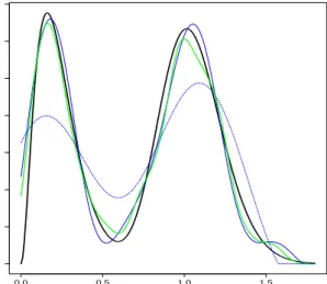
practice for the kernel estimator. We notice that this strategy produces very good results in practice, better than choosing the sameκ for the two apparitions of termV(h). On Figure 1 25 estimatorsfb
b
h are plotted and on Figure 2 25 estimatorsfem,e es, for the 4 investigated densities
f . The batch of estimators is close to the estimated density.
In order to evaluate the performances of each estimator on the different designs, we compare their empirical MISE computed from 100 simulated data sets.
Table 1 summarises the results for different parameters values. It shows the bad perfor-mances of the estimator of Comte et al. (2013) fe
e e
τ when T is small compared to fem,e es. It
performs clearly better when T is increasing. Besides we notice that both kernel estimators have good results. Nevertheless these results are satisfying because it appears that our esti-mator fb
bh fits slightly better the true density thanfbcv. The computation time is close for both
selection method. We show the results for different values of α do not seem to influence the quality of estimators (while the selectedh, m, sare very different). During the simulation study, we noticed that the parameter α is important is the sense that when the value ofα does not have the same order as the values of φ, the estimation is harder. Except when T = 300 the ratio signal noise which is the standard deviation of the random effect divided by σ is larger than one thus the settings are favourables. But for both gamma and mixed gamma cases, the standard deviations are respectively 0.2 and 0.15, which is not small compared toσ or to their mean. The mixed gamma case is difficult for the nonparametric estimation: Figure 3 illustrates the performances of estimators for this choice. Finally, it is interesting to note that when the standard deviation of the random effect of interest has a larger variance, the density estima-tion is easier, which is the case of the chosen gamma density for example compared with the Gaussian case.
In the following as the two kernel estimators seem very close, we only show the results for
b f
bh which is of interest here. Besides we no longer investigate the previous estimator
e f e e τ in light of Table 1 forT < N.
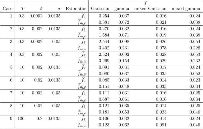
Table 1: Empirical MISE computed from 100 simulated data sets, withN = 200, with various
T,δ,σ andα for two kernel estimatorsfbcv,fb
b
h and two deconvolution estimators fbe e τ andfem,e es b fcv fb b h feeeτ e f e m,es Casef Gamma T = 0.3 δ= 0.0005σ = 0.0135α= 0.039 0.043 0.037 1.547 0.071 T = 300δ = 0.5 σ= 0.5 α= 39 0.048 0.039 0.049 0.055 T = 50δ = 0.1σ = 0.05 α= 1 0.042 0.039 0.218 0.050 Casef mixed Gamma
T = 0.3 δ= 0.0005σ = 0.0135α= 0.039 0.033 0.030 0.712 0.035
T = 300δ = 0.5 σ= 0.5 α= 39 0.032 0.030 0.035 0.043
T = 50δ = 0.1σ = 0.05 α= 1 0.033 0.031 0.145 0.043
We further compare fb
bh and fem,e es. The two estimators seem close to the true density on
graphs, see Figure 1 and 2. In Table 2 on the MISE it is clear that the kernel estimator is the best. Furthermore, we can point out some differences. The first row of the Table corresponds to simulations with the parameters of the real dataset. In the first column, the Gaussian case, the MISE are 10 times larger than the ones for other cases. This can be easily explained: the values of the estimated density are 10 times larger than others. Nevertheless, on lines 3 and 4 for the Gaussian case, the MISE are very large. This is due to the bad estimation of the φj by theZj,T with σ = 0.05 and T = 0.3 1. The quality of the estimation is significantly better when we try a N(0.278,0.2) (0.2 is the variance of the mixed Gaussian density we implement for example). In general one can notice that when σ is larger than the standard deviation of the density of the random effectsf, the estimation is less precise, which is coherent in term of signal to noise ratio.
Table 2 shows that if T increases, it improves the results for σ = 0.05, compare cases 2 and 5 with 4 and 7 for example. IfJ is large enough, meaning if δ is small enough (which is the case even forJ = 150 when T = 0.3), the deconvolution estimator fits well the density. In practice, whenT increases, the selected value of sdecreases, which could have been predicted. The results are still satisfying for large T. For the kernel estimator, although the theoretical condition1/h5< T2 is not satisfied, the numerical results are good.
Another point is, as expected, that the larger N is, the better the estimators fb
b
h and fe
e
m,es.
We can refer to Comte et al. (2013) for a study with different values for N. It highlights the influence ofN when the estimated density has two modes; for example with N = 50 the estimation is clearly less precise than forN = 200.
A main difference between our two estimators fb
b
h and fem,e es is the computation time: a few
seconds for the first one and ten minutes for the second one. Thus the kernel estimator with the method of bandwidth selection is very efficient, especially in the case of multi-modal densities, and performs often better than the deconvolution one.
1We insist that this bad estimation is not due to the fact that the noise is Gaussian. Indeed even if Fan
(1991) proves the rates to be logarithmic in that case, the rates are improved and can be polynomial when the density under estimation is of the same type as the noise (see Lacour (2006), Comteet al.(2006)).
(a)fGaussian (b)f mixed Gaussian density
(c) fGamma (d)f mixed Gamma density
Figure 1: Simulated data. In plain black (red) 25 estimators fb
b
h with parameters: N = 240,
(a)fGaussian (b) f mixed Gaussian
(c) fGamma (d) fmixed Gamma
Figure 2: Simulated data. In plain black (red) 25 estimators fe
e
m,es with parameters: N = 240,
T = 0.3, δ= 0.00015,σ= 0.0135,α= 0.039and the true densityf in bold plain black line
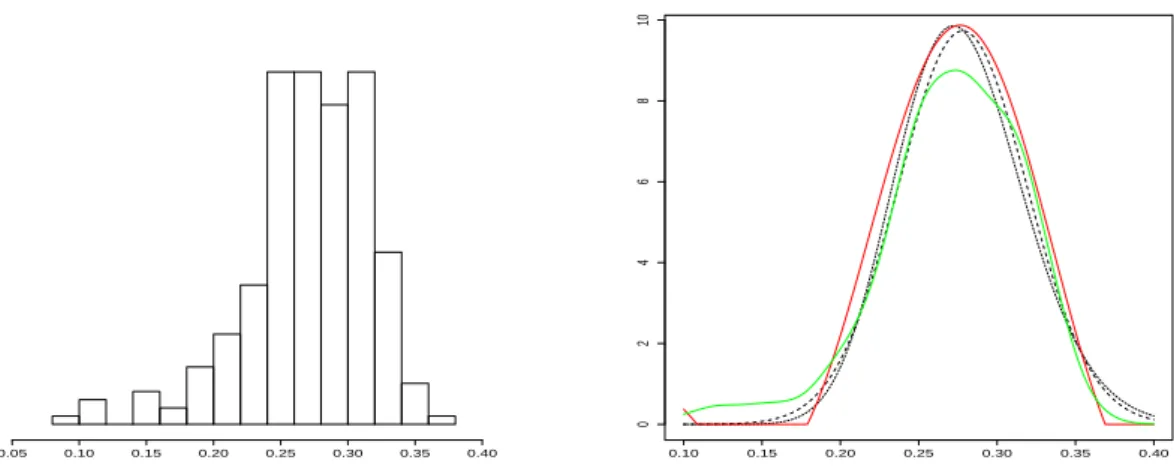
0.0 0.5 1.0 1.5 0.0 0.2 0.4 0.6 0.8 1.0 1.2 1.4
Figure 3: Simulated data. In bold plain black curve is the true density f mixed Gamma, the estimatorfbcv estimatorfb
b
h are superposed is in plain grey (green), estimatorfee e
τ is dotted black (blue) and estimator fe
e
m,es is plain black (blue), with N = 200, T = 50, δ = 0.05, σ = 0.05,
Table 2: Empirical MISE computed from 100 simulated data sets, with N = 240, α = 0.039
and variousT,δ,σ for the kernel estimatorfb
b
h and the deconvolution estimatorfem,e es
f
Case T δ σ Estimator Gaussian gamma mixed Gaussian mixed gamma 1 0.3 0.0002 0.0135 fb b h 0.254 0.037 0.016 0.024 e f e m,es 0.381 0.072 0.021 0.038 2 0.3 0.002 0.0135 fb b h 0.270 0.032 0.016 0.024 e f e m,es 1.584 0.071 0.019 0.038 3 0.3 0.0002 0.05 fb b h 2.544 0.098 0.026 0.054 e f e m,es 3.402 0.231 0.078 0.226 4 0.3 0.002 0.05 fb b h 2.524 0.092 0.028 0.053 e f e m,es 3.269 0.154 0.029 0.232 5 10 0.002 0.0135 fb b h 0.091 0.031 0.017 0.024 e f e m,es 0.080 0.037 0.035 0.052 6 10 0.02 0.0135 fb b h 0.085 0.033 0.014 0.023 e f e m,es 0.151 0.048 0.033 0.034 7 10 0.002 0.05 fb b h 0.111 0.031 0.016 0.025 e fm,e es 0.687 0.061 0.016 0.034 8 10 0.02 0.05 fb b h 0.121 0.035 0.014 0.025 e f e m,es 0.181 0.053 0.023 0.040 9 100 0.2 0.0135 fb b h 0.106 0.032 0.014 0.024 e f e m,es 0.123 0.062 0.091 0.046
6
Application to neuronal data
6.1 Dataset
We describe quickly the data but we refer to Yuet al.(2004); Lanskyet al.(2006) for example for details on data acquisition. The data are intracellular measurements of the membrane potential in volts along time, for one single neuron of a pig between the spikes. This is the depolarization phase. In this neuronal context, between the (j−1)th and the jth spike, the depolarization of the membrane potential receiving a random input can be described by the Ornstein Uhlenbeck model with one random effect (1). The spikes are not intrinsic to the model but are generated when the voltage reaches for the first time a certain thresholdS, then the process is reset to a fixed initial voltage. Thus each trajectory is observed on an interval
[0, Tj] where Tj = inf{t > 0, Xj(t) ≥ S}. The initial voltage (the value following a spike) is assumed to be equal to the resting potential. The present dataset has been normalised to obtain
N trajectories which begin in zero: xj = 0.
The positive constant parameterαis called the time constant of the neuron (the coefficient of decay in the exponential, when there is no noise), which is intrinsic to the neuron and fixed to α = 0.039 [s] (Lansky et al., 2006). The diffusion coefficient σ [V/√s]has been estimated using the estimator cσ2 = (1/N)PN
j=1 (1/J)PJ k=1((Xj(δ(k+ 1))−Xj(δk))2/δ . We obtain
σ = 0.0135, which is the same value as that used in Picchini et al. (2008). The φj represents the local average input that the neuron receives during thejth inter-spike interval. We assume that φj changes from one trajectory to another because of other neurons or the influence of the environment, for example. So parametersφand σ characterize the input, whileα, xj (the resting potential) andS (the firing threshold) describe the neuron irrespectively of the incoming signal (Picchiniet al., 2008).
Data are composed of N = 312 inter-spike trajectories. For each interval [0, Tj] the time step is the same: δ = 0.00015 [s]. We decide to keep only realizations with more than 2000 observations (Tj/δ ≥2000). Finally we haveN = 240 realizations withJ = 2000 observations and for j = 1, . . . , N, T =Tj = 0.3 [s]. Also the data are normalized in order to begin with zero at the initial time. The study of the units of measurement can highlight the collections given in Section 4. One can notice that the unit of measurement ofv in the integrand must be
[s/V] (same unit as1/Zj,τ) such that the exponential terms are without unit. The unit of sis
[√s/V], and the choice ofMwith the same unit asv seems natural.
In is interesting to note that the normality of theZj,T is rejected by Shapiro and Wilk test (p-value 10−7) and Kolmogorov-Smirnov test (p-value 10−3). This suggests that the φ
j’s are not Gaussian. Thus we want to estimate nonparametrically their density. In the following we compare our results to the estimation obtained in Picchiniet al. (2010) under the parametric Gaussian assumption.
6.2 Comparison of estimators
The estimation of the densityf obtained by Picchiniet al.(2010) under the Gaussian assump-tion on these data areN(µ= 0.278, η2= (0.041)2). Using a maximum-likelihood estimator on
the(Zj,T)’s we obtain for the mean 0.270 and for the standard deviation 0.046. We notice that these two estimations are close to that of Picchiniet al. (2010) even if theZj,T are noisy when
T is small. We use our two nonparametric estimators to see how close to a Gaussian density they are.
On Figure 4 we represent both estimators fb
b
h and fem,ese applied on the real data and the
(2010). However, it is also legitimate to think about a Gamma distribution to model the random parametersφj’s because, as the data have been normalised, the estimated random effects are positive. Then it seems reasonable to use a non-negative random variable to model this local average input. Thus, a Gamma distribution may seem more appropriate than a Gaussian distribution, even if the chosen Gaussian has small probability to be negative. We look for the Gamma distribution which has for meanµ= 0.278and for standard deviation η= 0.041. This corresponds to a Gamma distribution with the shape parameter 46.3 and the scale parameter
0.006. We notice the similarity between the previous Gaussian curve and the new one. Thus this distribution seems also suitable to fit the distribution of theφj’s, as Figure 4 shows.
The Gaussian assumption is strong and leads to parametric tractable models. The present work confirms that this approximation is acceptable. However, the nonparametric estimation gives a density for theφj’s that can be used to simulate the random effect and could be closer to the true one.
Notice that, as mentioned in introduction, Comte et al. (2013)’s estimator cannot handle small values ofT while our new proposals are successful in such case. Let us precise this point. The Zj,T ≈ Xj(T)−Xj(0) + δ α J X l=1 X((l−1)δ) ! 1 T
is unchanged when we change the units: V,s to mV,ms thus T = 0.3to T = 300. However, the deconvolution estimator of Comte et al. (2013) for τ = T is changing when the value of T is changing. In fact, the estimator is
b fT(x) = 1 2π Z √ T −√T e−iux1 N N X j=1 eiuZj,Teu 2σ2 2T du ≈ 1 2π npas X k=1 (uk+1−uk)e−iukx 1 N N X j=1 eiukZj,Te u2kσ2 2T
and according to T = 0.3 or T = 300 the values of u and thus the interval of integration and the three exponential terms are changing. Finally estimatorfbT is changing with the units. And
the interval of integration is not large enough in the caseT = 0.3to gave a good estimation. To solve this problem we have proposed a new estimatorfe
e
m,esto allow the user to deal with
data with the units he/she wants and to not oblige him/her to change it.
But one can wonder if the new estimators are robust when increasingT. Indeed, our method works for larger T. Precisely changing volts in millivolts and seconds in milliseconds implies
T = 300,σ = 0.426, and on simulated data we adequately reconstruct the shape of the density.
7
Discussion
In this work we study a stochastic differential Ornstein-Uhlenbeck mixed-effects model. We propose two estimators of the density of the random effect. Both estimators are not very sensitive to the effect of the time of observationT. Indeed the kernel strategy corresponds to a context with large T while we built a deconvolution estimator especially for small values of T. Both are data-driven and satisfy an oracle-type inequality. According to the numerical study, the kernel estimator seems to be the efficient one: the numerical results are convincing and close to the ones obtained by cross-validation. Besides we provide non-asymptotic theoretical results. Furthermore we study neuronal data with nonparametric estimation strategy. Instead
0.05 0.10 0.15 0.20 0.25 0.30 0.35 0.40 0 2 4 6 8 10 0.10 0.15 0.20 0.25 0.30 0.35 0.40 0 2 4 6 8 10
Figure 4: Real data. In green estimatorfb
b
h, in redfem,e es, the black dotted and bold line the density
N(µ, η2)from Picchini et al. (2010) and the black dotted thin line the densityΓ(46.3,0.006)
of making any parametric assumptions for the random effect distribution, we build an estimator of its density. Future work based on this estimation could be more precise and closer to the real neuronal data. To complete the study, the method for different times of observation Tj could be settled up. Besides, some goodness-of-fit tests could be produced; we refer to Bissantz
et al. (2007) who construct confidence bands for an estimator of f in the ordinary smooth deconvolution problem.
The model can be completed by adding another random effect: the time constant of the neuron. Picchini and Ditlevsen (2011) have investigated this model in a parametric way and Dion and Genon-Catalot (2015) in a nonparametric way. A recent work Delattre et al. (2015) assumes that the density of the random effect is a Gaussian mixture and uses data clustering method, which is an interesting approach for the data described in the present paper. The question of a random effect in the diffusion coefficient also is open (see Delattreet al. (2014)). Moreover, a model with a driftb(Xj(t)) +φj, where bis a known function, can be treated with the same method. However, dealing with a diffusionσ(Xj(t))whereσ is a known function is a more complex problem.
AcknowledgementsThe author would like to thank Fabienne Comte and Adeline Samson for very useful discussions and advice.
8
Proofs
8.1 Proof of Theorem 2 Givenh∈ HN,T, we denote: V(h) =κ1 kKk2 1kKk2 N h +κ2 σ4kKk2 1kK00k2 T2h5 =:V1(h) +V2(h).Using the definition ofA(h) and ofbh we obtain kfb b h−fk 2 ≤ 3k b f b h−fbh,bhk 2+ 3k b fh, bh−fbhk 2+ 3k b fh−fk2 ≤ 3 A(h) +V(bh) + 3 A(bh) +V(h) + 3kfbh−fk2 ≤ 6A(h) + 6V(h) + 3kfbh−fk2.
Thus, E[kfb b h−fk 2]≤6 E[A(h)] + 6V(h) + 3E[kfbh−fk2],
hence, we only have to study the termE[A(h)]. We can decomposekfbh,h0 −fbh0k2 as follows:
kfbh,h0−fbh0k2≤5kfbh,h0−E[fbh,h0]k2+5kE[fbh,h0]−fh,h0k2+5kfh,h0−fh0k2+5kfh0−E[fbh0]k2+5kE[fbh0]−fbh0k2 thus A(h)≤5(D1+D2+D3+D4+D5) with: D1 := sup h0∈H N,T kfh,h0−fh0k2, D2:= sup h0∈H N,T kfbh0 −E[fbh0]k2− V1(h0) 10 + , D3 := sup h0∈H N,T kfbh,h0 −E[fbh,h0]k2− V1(h0) 10 + D4 := sup h0∈H N,T kE[fbh0]−fh0k2− V2(h0) 10 + , D5 := sup h0∈H N,T kE[fbh,h0]−fh,h0k2− V2(h0) 10 + .
According to Young’s inequality (see Theorem 7), we obtain
kfh,h0 −fh0k2 =kKh0 ?(fh−f)k2 ≤ kKh0k21kfh−fk2 =kKk21kfh−fk2
thus
D1 ≤ kKk21kfh−fk2. (18) Let us study the termD2. We denoteB(1) ={g∈L2(R),kgk= 1}. We define
νN,h(g) :=< g,fbh−E[fbh]>
then|νN,h(g)| ≤ kgkkfbh−E[fbh]k thus, the estimatorfbh satisfies:
kfbh−E[fbh]k2= sup
g∈B(1)
(νN,h(g))2.
We can also compute the scalar product which definesνN,h and we obtain
νN,h(g) = 1 N N X j=1 g ? Kh−(Zj,T)−E[g ? Kh−(Zj,T)] (19)
withKh−(x) :=Kh(−x). This finally conducts to:
E[D2]≤ X h0∈H N,T E " sup g∈B(1) (νN,h0(g))2−V1(h 0) 10 # + .
This bound and Equation (19) leads to apply Talagrand’s Theorem (8). We have to compute 3 quantities: M,H2 and v.
First: sup g∈B(1) kg ? Kh−0k∞ = sup g∈B(1) sup x∈R Z g(y)Kh−0(x−y)dy = sup g∈B(1) sup x∈R |< g, Kh−0(.−x)>| ≤ sup g∈B(1) kgkkKh0k= kKk √ h0 :=M. (20)
Secondly, the bound of Proposition 1 gives
E " sup g∈B(1) (νN,h(g))2 # =E[kfbh−E[fbh]k2]≤ kKk2 N h :=H 2. (21) Thirdly: sup g∈B(1) Var(g ? Kh−0(Z1,T)) ≤ sup g∈B(1) E[(g ? Kh−0(Z1,T))2] ≤ 2 sup g∈B(1) E[(g ? Kh−0(φ1))2] + 2 sup g∈B(1) E[(g ?(Kh−0(Z1,T)−Kh−0(φ1))2].
Let us investigate the two terms separately. Young’s inequality gives:
E[(g ? Kh−0(φ1))2] = Z (g ? Kh−0(x))2f(x)dx≤ kfkkg ? Kh−0k24 = kfkkKk2 4/3 √ h0 :=v1. (22)
Then, one can write: Kh0(x−Z1,T)−Kh0(x−φ1) = (φ1−Z1,T)R1
0(Kh0) 0(x−φ 1+u(φ1−Z1,T))du, thus (g ? Kh−0(Z1,T)−g ? Kh0(φ1))2 = (φ1−Z1,T)2 Z g(x) Z 1 0 (Kh0)0(x−φ1+u(φ1−Z1,T))dudx 2 ≤ (φ1−Z1,T)2 Z g2(x) Z 1 0 (Kh0)02(x−φ1+u(φ1−Z1,T))du dx ≤ (φ1−Z1,T)2kgk2 Z (Kh0)02(y)dy= (φ1−Z1,T)2k(Kh0)0k2. WithE[(φ1−Z1,T)2] = σ 2 T2E[W1(T)2] = σ 2 T , the assumptionT −1 ≤h5/2 leads to E[(g ? Kh−0(Z1,T)−g ? Kh0(φ1))2]≤ kK0k2σ2 h03T ≤ kK0k2σ2 √ h0 :=v2. (23) Finallyv=v1+v2 =A0/ √ h0 withA 0=kfkkKk24/3+kK0k2σ2.
Ifκ1kKk21 ≥40, with the assumption1/(N h) ≤1, Talagrand’s inequality (under the
assump-tions of the Theorem 2) gives
E sup g∈B(1) (νN,h0(g))2−V1(h 0) 10 ! + ≤ C1 N√h0e −C2/ √ h0 +C3 1 h0N2e −C4 √ N ≤ C5 N X h0∈H N,T 1 √ h0e −C6/ √ h0 ≤ C5S(C6) N .
One can lead the study of D3 as we have done for D2, using the same steps and tools.
HoweverKh? Kh0 instead of Kh0, addskKk1 inM andkKk21 inH2 andv.
Then, let us study the termD4. Ifκ2≥10/(3kKk21), the bound (9) leads us to
D4 = sup h0∈H N,T kE[fbh0]−fh0k2− V2(h0) 10 + ≤ sup h0∈H N,T k K00k2σ4 3h05T2 − κ2kKk21kK00k2σ4 10T2h05 + = 0
thusD4 = 0. Finally, similarly, if κ2 ≥10/3, we obtain
D5 = sup h0∈H N,T kE[fbh,h0]−fh,h0k2− V2(h0) 10 + ≤ sup h0∈H N,T kK00k2kKk2 1σ4 3h5T2 − κ2kKk21kK00k2σ4 10T2h05 + = 0.
Thus finally we obtained that:
E[A(h)]≤5 kKk21kfh−fk2+ c N (24) with c a constant depending on kfk,kKk1,kKk,kKk4/3. Finally we have shown that for all
h∈ HN,T: E[kfb b h−fk 2] ≤ 6κ 1 kKk2 1kKk2 N h + 6κ2 kKk2 1kK00k2σ4 T2h5 + 3 2kf −fhk2+ kKk2 N h + 2kK00k2σ4 3T2h5 + 30kKk2 1kf−fhk2+ c N ≤ 6 + 3 kKk2 1κ1 V1(h) + 6 + 9 2kKk2 1κ2 V2(h) + (30kKk21+ 6)kfh−fk2+ C N ≤ C1 inf h∈HN,T {kf −fhk2+V(h)}+ C2 N.
whereC1 = max(7,30kKk12+ 6)and C2 depends on kfk,kKk1,kKk,kKk4/3.
8.2 Proof of Proposition 3
The bias term iskf−E[fem,s]k2. Let us computeE[fem,s]. As theZj,τ arei.i.d.. whenτ is fixed
and due to the independence ofφ1 and W1, we obtain:
E[fem,s(x)] = 1 2π Z m −m e−iuxE h eiuZ1,m2/s2+u 2σ2s2/(2m2)i du = 1 2π Z m −m e−iuxE h eiuφ1+iuσW1(m2/s2)s2/m2+u2σ2s2/(2m2)idu = 1 2π Z m −m e−iux+u2σ2s2/(2m2)f∗(u)E h eiuσW1(m2/s2)s2/m2idu = 1 2π Z m −m e−iux+u2σ2s2/(2m2)f∗(u)e−u2σ2s2/(2m2)du = 1 2π Z m −m e−iuxf∗(u)du=:fm(x).
Therefore this givesE[fem,s(x)] =fm(x), andkf−E[fem,s]k2=kf−fmk2 = 21π R
|u|≥m|f
∗(u)|2du.
The variance term is:
E h kfem,s−fmk2 i = 1 2πE Z m −m 1 N N X j=1 eiuZj,m2/s2eu 2σ2s2 2m2 −f∗(u) 2 du = 1 2πN Z m −m eu 2σ2s2 m2 Var eiuZ1,m2/s2du ≤ 1 2πN Z m −m eu 2σ2s2 m2 du= m πN Z 1 0 es2σ2v2du. 8.3 Proof of Theorem 5
Let us study the termkfe
e
m,es−fk
2. We decompose it into a sum of three terms and the definition
of(m,e es) (15) implies for all(m, s)∈ C kfe e m,es−fk 2 ≤ 3k e fm,e es−fe(m,ees)∧(m,s)k 2+k e f(m,e es)∧(m,s)− e fm,sk2+kfem,s−fk2 ≤ 3 (Γm,s+pen(m,e es)) + 3 Γm,e es+pen(m, s) + 3kfem,s−fk2 ≤ 6Γm,s+ 6pen(m, s) + 3kfem,s−fk2 (25)
Now we studyΓm,s. First:
kfe(m,s)∧(m0,s0)−fem0,s0k2≤3 kfem0,s0 −fm0k2+kfm0−fm∧m0k2+kfm∧m0−fe(m0,s0)∧(m,s)k2 . Thus: Γm,s ≤ max (m0,s0)∈C 3kfem0,s0−fm0k2+ 3kfm0 −fm∧m0k2+ 3kfm∧m0−fe(m0,s0)∧(m,s)k2−pen(m0, s0) + ≤ 3 max (m0,s0)∈C kfem0,s0−fm0k2−1 6pen(m 0, s0) + + 3 max (m0,s0)∈C kfe(m0,s0)∧(m,s)−fm∧m0k2−1 6pen(m 0, s0) + + 3 max m0∈Mkfm 0 −fm∧m0k2.
The last maximum can be explicit. If m0 ≤ m, then kfm0 −fm∧m0k2 = kfm0 −fm0k2 = 0.
Otherwise, kfm0 −fm∧m0k2=kfm0 −fmk2 = Z m≤|u|≤m0 |f∗(u)|2du≤ kf −fmk2. Finally: max m0∈Mkfm 0 −fm∧m0k2 ≤ kf−fmk2.
Γm,s ≤ 3 max (m0,s0)∈C kfem0,s0−fm0k2− 1 6pen(m 0, s0) + + 3 max (m0,s0)∈C kfe(m0,s0)∧(m,s)−fm∧m0k2−1 6pen(m 0, s0) + + 3kf −fmk2. (26)
Then we gather Equations (25) and (26):
kfe e m,es−fk 2 ≤ 6pen(m, s) + 3k e fm,s−fk2+ 18kf −fmk2+ max (m0,s0)∈C18 kfem0,s0−fm0k2− 1 6pen(m 0, s0) + + max (m0,s0)∈C18 kfe(m0,s0)∧(m,s)−fm∧m0k2− 1 6pen(m 0, s0) + .
We first notice that our penalty function is increasing in s and m, thus we get the following bound for the last term:
E " max (m0,s0)∈C kfe(m0,s0)∧(m,s)−fm∧m0k2− 1 6pen((m 0, s0)∧(m, s)) + # ≤ E " max m0≤m,s0≤s kfem0,s0−fm0k2− 1 6pen(m 0, s0) + # +E " max m≤m0,s≤s0 kfem,s−fmk2− 1 6pen(m, s) + # +E " max m≤m0,s0≤s kfem,s0−fmk2− 1 6pen(m, s 0) + # +E " max m0≤m,s≤s0 kfem0,s−fm0k2− 1 6pen(m 0, s) + # ≤ 4 X m0∈M X s0∈S E kfem0,s0−fm0k2− 1 6pen(m 0, s0) + .
Moreover, according to Proposition 3 and using the inequalityR01eσ2s2v2dv≤eσ2s2, we obtain, for all
(m, s)∈ C, E[kfe e m,es−fk 2] ≤ 5×18 X m0∈M X s0∈S E kfem0,s0−fm0k2− 1 6pen(m 0, s0) + + 6pen(m, s) + 3 m πNe σ2s2+ 21kf −f mk2.
Then we obtain the announced result with the following Lemma.
Lemma 6 There exists a constant C0 >0such that for pen(m, s) defined by pen(m, s) =κmNeσ2s2,
X m0∈M X s0∈S E kfem0,s0−fm0k2− 1 6pen(m 0, s0) + ≤C 0(P+ 1) N .
According to Lemma 6, to be proved next, we choose pen(m, s) = κmNeσ2s2, thus, there exist two
constantsC= 145, C0 >0 such that,
E[kfe e m,es−fk2] ≤ 5×18 X m0∈M X s0∈S E kfem0,s0−fm0k2− 1 6pen(m 0, s0) + + (6κ+3 π) m Ne σ2s2+ 21kf −f mk2 ≤ C inf (m,s)∈C{kf−fmk 2+m Ne σ2s2 }+C 0 N.
Proof of Lemma 6
For a couple(m, s)∈ Cfixed, let us consider the subsetSm:={t∈L1(R)∩L2(R),supp(t∗) = [−m, m]}.
Fort∈Sm, νN(t) = 1 N N X j=1 ϕt(Zj,m2/s2)−E[ϕt(Zj,m2/s2)] withϕt(x) := 21πR t∗(u)eiux+σ 2u2s2/(2m2)
du, thenνN(t) =21π < t∗,(fem,s−fm)∗>. This leads to
kfem,s−fmk2= sup t∈Sm,ktk=1
|νN(t)|2. (27)
We also have by Cauchy-Schwarz inequality kϕtk∞ ≤ 1 2π Z |t∗(u)|eσ2u2s2/(2m2)du≤ 1 2π Z m −m |t∗(u)|2du 1/2Z m −m eσ2u2s2/m2du 1/2 ≤ √ 2m √ 2πe σ2s2/2 thus sup t∈Sm,ktk=1 kϕtk∞≤ √ m √ πe σ2s2/2 :=M. Then, by Proposition 3, E " sup t∈Sm,ktk=1 |νN(t)|2 # =Ehkfem,s−fmk2 i ≤ m πN Z 1 0 eσ2s2v2dv≤ m πNe σ2s2 :=H2.
Using Fubini and Cauchy-Schwarz inequalities we obtain for all(m, s)∈ C:
4π sup t∈Sm,ktk=1 Var(ϕt(Zj,m2/s2)) ≤ sup t∈Sm,ktk=1 Z Z t∗(u)t∗(−v)E h ei(u−v)Zj,m2/s2ie(u2+v2)σ2s2/(2m2)dudv ≤ 2π Z Z [−m,m]2 |f∗(u−v)|2e(u2+v2)σ2s2/m2dudv !1/2 ≤ 2π e2σ2s2 Z Z [−m,m]2 |f∗(u−v)|2dudv !1/2 ≤ 2πeσ2s2√2m( Z 2m −2m |f∗(z)|2dz)1/2≤2√2m√2π√πeσ2s2kfk=: 4π2v, v:= √ meσ2s2kfk √ π .
Finally using that m ≤ N, s ≤ 2/σ and P
s∈Ss = (4/σ)(1−(1/2)P+1) < 4/σ, the Talagrand’s inequality withα= 1/2 if4H2≤pen(m, s)/6implies,
X s∈S X m∈M E kfem,s−fmk2− 1 6pen(s, m) + ≤X s∈S X m∈M C 1kfk N e σ2s2√ me−C2 √ m kfk+C 3 m N2e σ2s2 e−C4 √ N ≤ X s∈S C1kfk N e σ2s2 X m∈M √ me−C2 √ m kfk ! +X s∈S X m∈M C3e4 1 Ne −C4 √ m ≤ C1kfk(P+ 1)e 4 N X m∈M √ me−C2 √ m kfk ! +C3e4 P+ 1 N X m∈M e−C4 √ m ≤ C 0(P+ 1) N
because with the definition ofM,P m∈M √ me−C2 √ m kfk ≤a 1Pk∈Nk 1/4e−a2k1/4 <+∞, andP m∈Me− C4m1/2 ≤ P k∈Ne −a3k1/4 <+∞, witha
1, a2, a3 three positive constants. Notice thatC0 >0 depends on σ,kfk,
∆.
We choose pen(m, s) =κmeσ2s2/N withκ≥24.
A
Appendix
A.1 Young inequality
This inequality can be found in Briane and Pagès (2006) for example.
Theorem 7 Letf be a function belonging toLp(R)andgbelonging toLq(R), letp, q, rbe real numbers
in[1,+∞]and such that
1 p+ 1 q = 1 r + 1. Then, kf ? gkr≤ kfkpkgkq.
A.2 Talagrand’s inequality
The following result follows from the Talagrand concentration inequality given in Klein and Rio (2005) and arguments in Birgé and Massart (1998).
Theorem 8 Consider n∈N∗,F a class at most countable of measurable functions, and(Xi)i∈{1,...,N}
a family of real independent random variables. One defines, for allf ∈ F,
νN(f) = 1 N N X i=1 (f(Xi)−E[f(Xi)]).
Supposing there are three positive constantsM,H andv such that sup f∈F kfk∞≤M, E[sup f∈F |νNf|]≤H, and sup f∈F (1/N)PN
i=1Var(f(Xi))≤v, then for all α >0,
E " sup f∈F |νN(f)|2−2(1 + 2α)H2 ! + # ≤ 4 a v N exp −aαN H 2 v + 49M 2 aC2(α)N2exp − √ 2aC(α)√α 7 N H M !! withC(α) = (√1 +α−1)∧1, anda= 16. A.3 Discretization
Indeed, if we assume that the times of observations are the tk =kδ, k = 1, . . . , N and0 < δ < 1, we
must study the error applied by discretization of theZj,τ. Then, for any0< m2/s2≤T we use:
b Zj,m2/s2 = s2 m2 Xj(δ[m2/(s2δ)])−Xj(0) + δ α [m2/(s2δ)] X k=1 Xj((k−1)δ) (28)
to approximateZj,m2/s2 given by (2). The corresponding estimator off is
be fm,s(x) = 1 2π Z m −m e−iux 1 N N X j=1 eiuZbj,m2/s2eu 2σ2s2 2m2 du. (29)
We investigate the error: E[kfbe m,s−fk 2]≤2 E[kfbe m,s−fem,sk2] + 2E[kfem,s−fk2]
where the second term of the right hand side is bounded by Proposition 3. Then, Plancherel-Parseval’s Theorem implies: E[kb e fm,s−fem,sk2] ≤ 1 2πE Z m −m 1 N N X j=1 eu2σ2s2/m2 e iuZbj,m2/s2 −eiuZj,m2/s2 2 du ≤ 1 2π Z m −m eu2σ2s2/m2E e iuZb1,m2/s2−eiuZ1,m2/s2 2 du and E e iuZb1,m2/s2 −eiuZ1,m2/s2 2 ≤ |u|2 E Zb1,m2/s2−Z1,m2/s2 2
thus we study the last term. For all(m, s)∈ C,m2/s2≤T,
Z1,m2/s2−Zb1,m2/s2 = s2 m2 Xj(m 2/s2)−X j(δ[m2/(s2δ)]) + s 2 αm2 [m2/(s2δ)] X k=1 Z kδ (k−1)δ (Xj(s)−Xj((k−1)δ))ds
then by Cauchy-Schwarz’s inequality we obtain
(Z1,m2/s2−Zb1,m2/s2)2 ≤ 2s4 m4 Xj(m 2/s2)−X j(δ[m2/(s2δ)]) 2 + 2s 4 α2m4 [m2/(s2δ)] X k=1 Z kδ (k−1)δ (Xj(s)−Xj((k−1)δ))ds 2 .
Höder’s inequality yields hm2 s2δ i X k=1 Z kδ (k−1)δ (Xj(s)−Xj((k−1)δ))ds 2 ≤ hm2 s2δ i X k=1 " Z kδ (k−1)δ (Xj(s)−Xj((k−1)δ))ds #2 m2 s2δ ≤ m2 s2δ δ h m2 s2δ i X k=1 Z kδ (k−1)δ (Xj(s)−Xj((k−1)δ))2ds.
Let us studyE[(Xj(s)−Xj((k−1)δ))2], for(k−1)δ≤s≤kδ:
Xj(s)−Xj((k−1)δ) = Z s (k−1)δ φj− Xj(u) α du+ Z s (k−1)δ σdWj(u)
and Cauchy-Schwarz’s inequality gives
E[(Xj(s)−Xj((k−1)δ))2] ≤ 2E Z s (k−1)δ φj− Xj(u) α du !2 + 2E Z s (k−1)δ σdWj(u) !2 ≤ 2E " Z s (k−1)δ φj− Xj(u) α 2 du # + 2δσ2 ≤ 4δ2 E(φ2j) + 1 α2sup s≥0E [Xj(s)2] + 2δσ2. (30)
Finally, after simplification and using for allx∈R+,[x]≤x, E h (Z1,m2/s2−Zb1,m2/s2)2 i ≤ 2s 4 m4E[ Xj(m 2/s2) −Xj(δ[m2/(s2δ)]) 2 ] + 2 α2 4δ2 E(φ2j) + 1 α2sup s≥0E [Xj(s)2] + 2δσ2
and we can deal with the term E[ Xj(m2/s2)−Xj(δ[m2/(s2δ)])
2
] using formula (30) and m2/s2−
δ[m2/(s2δ)]≤δ. Thus: E h (Z1,m2/s2−Zb1,m2/s2)2 i ≤ 2s4 m4 + 2 α2 4δ 2 E(φ2j) + 1 α2sup s≥0E [Xj(s)2] + 2δσ2 .
Besides, for model (1), Equation (17) implies E[Xj(s)2] ≤ 3x2j + 3α
2 E[φ2j] + 3σ 2, and 0 < δ < 1 implies E h (Z1,m2/s2−Zb1,m2/s2)2 i ≤ Cδ 2s4 m4 + 2 α2
withCa positive constant which does not depend onδorm2/s2. Finally,
E[kb e fm,s−fem,sk2] ≤ Cδ 2s4 m4 + 2 α2 1 2π Z m −m u2eu2σ2s2/m2du ≤ C0δ Z 1 0 v2ev2σ2s2dv s 4 m + m3 α2 .
Buts≤2/σandm=√k∆/σ, withk∈N∗ and0<∆<1, thus we obtain
E[kb e fm,s−fem,sk2] ≤ C0 σ3 Z 1 0 v2ev2σ2s2dv 24√k δ √ ∆ +k 3/2 α2 δ∆3/2 .
Proposition 9 Under (A), assumingE[φ2j]<+∞, the estimatorbfem,s given by (29) satisfies
E h kfem,s−fk2 i ≤ kfm−fk2+ √ k∆ σπNe σ2s2 +C 0 σ3 eσ2s2 2σ2s2 24√k δ √ ∆ +k 3/2 α2 δ∆3/2 .
Finally if∆ is fixed andδ is small, the error is acceptable. For example ifδ= ∆ the error is of order √
δ.
For study on the kernel estimator we refer to Comteet al.(2013).
References
Birgé, L. and Massart, P. (1998). Minimum contrast estimators on sieves: exponential bounds and rates of convergence. Bernoulli 4, 329–375.
Bissantz, N., Dümbgen, L., Holzmann, H. and Munk, A. (2007). Nonparametric confidence bands in deconvolution density estimation. Journal of the Royal Statistical Society: Series B (Statistical Methodology)69, 483–506.
Butucea, C. and Tsybakov, A. (2007). Sharp optimality in density deconvolution with dominating bias. II. Teor. Veroyatnost. i Primenen.52, 336–349.
Carroll, R. and Hall, P. (1988). Optimal rates of convergence for deconvolving a density. Journal of the American Statistical Association 83, 1184–1186. ISSN 01621459.
Chagny, G. (2013). Warped bases for conditional density estimation.Mathematical Methods of Statistics 22, 253–282.
Comte, F., Genon-Catalot, V. and Rozenholc, Y. (2007). Penalized nonparametric mean square estima-tion of the coefficients of diffusion processes. Bernoulli 13, 514–543.
Comte, F., Genon-Catalot, V. and Samson, A. (2013). Nonparametric estimation for stochastic differ-ential equation with random effects. Stochastic Processes and their Applications 7, 2522–2551. Comte, F. and Johannes, J. (2012). Adaptive functional linear regression. The Annals of Statistics 40,
2765–2797.
Comte, F., Rozenholc, Y. and Taupin, M.-L. (2006). Penalized contrast estimator for adaptive density deconvolution. Can. J. Stat.34, 431–452.
Comte, F. and Samson, A. (2012). Nonparametric estimation of random-effects densities in linear mixed-effects model. J. Nonparametr. Statist.24, 951–975.
Davidian, M. and Giltinan, D. (1995). Nonlinear models for repeated measurement data. Chapman and Hall.
Delattre, M., Genon-Catalot, V. and Samson, A. (2014). Estimation of population parameters in stochas-tic differential equations with random effects in the diffusion coefficient. Preprint MAP5-2014-07 . Delattre, M., Genon-Catalot, V. and Samson, A. (2015). Mixtures of stochastic differential equations
with random effects: application to data clustering Preprint MAP5-2015-36 .
Delattre, M. and Lavielle, M. (2013). Coupling the SAEM algorithm and the extended Kalman filter for maximum likelihood estimation in mixed-effects diffusion models. Statistics and Its Interface 6, 519–532.
Diggle, P., Heagerty, P., Liang, K. and Zeger, S. (2002).Analysis of longitudinal data. Oxford University Press.
Dion, C. and Genon-Catalot, V. (2015). Bidimensional random effect estimation in mixed stochastic differential model. Stochastic Inference for Stochastic Processes .
Donnet, S., Foulley, J. and Samson, A. (2010). Bayesian analysis of growth curves using mixed models defined by stochastic differential equations. Biometrics66, 733–741.
Donnet, S. and Samson, A. (2008). Parametric inference for mixed models defined by stochastic differ-ential equations. ESAIM P&S 12, 196–218.
Donnet, S. and Samson, A. (2013). A review on estimation of stochastic differential equations for pharmacokinetic - pharmacodynamic models. Advanced Drug Delivery Reviews 65, 929–939. Donnet, S. and Samson, A. (2014). Using PMCMC in EM algorithm for stochastic mixed models:
theoretical and practical issues. Journal de la Société Française de Statistique 155, 49–72.
Fan, J. (1991). On the optimal rates of convergence for nonparametric deconvolution problems. Ann. Statist.19, 1257–1272.
Genon-Catalot, V. and Jacod, J. (1993). On the estimation of the diffusion coefficient for multi-dimensional diffusion processes. Annales de l’institut Henri Poincaré (B) Probabilités et Statistiques 29, 119–151.