University of Wollongong University of Wollongong
Research Online
Research Online
Faculty of Engineering and Information
Sciences - Papers: Part B Faculty of Engineering and Information Sciences
2018
Modelling Group Heterogeneity for Small Area Estimation Using
Modelling Group Heterogeneity for Small Area Estimation Using
M-Quantiles
M-Quantiles
James DawberUniversity of Southampton, [email protected]
Raymond L. Chambers
University of Wollongong, [email protected]
Follow this and additional works at: https://ro.uow.edu.au/eispapers1
Part of the Engineering Commons, and the Science and Technology Studies Commons
Recommended Citation Recommended Citation
Dawber, James and Chambers, Raymond L., "Modelling Group Heterogeneity for Small Area Estimation Using M-Quantiles" (2018). Faculty of Engineering and Information Sciences - Papers: Part B. 1824.
https://ro.uow.edu.au/eispapers1/1824
Modelling Group Heterogeneity for Small Area Estimation Using M-Quantiles
Modelling Group Heterogeneity for Small Area Estimation Using M-Quantiles
Abstract Abstract
Small area estimation typically requires model-based methods that depend on isolating the contribution to overall population heterogeneity associated with group (i.e. small area) membership. One way of doing this is via random effects models with latent group effects. Alternatively, one can use an M-quantile ensemble model that assigns indices to sampled individuals characterising their contribution to overall sample heterogeneity. These indices are then aggregated to form group effects. The aim of this article is to contrast these two approaches to characterising group effects and to illustrate them in the context of small area estimation. In doing so, we consider a range of different data types, including continuous data, count data and binary response data.
Disciplines Disciplines
Engineering | Science and Technology Studies
Publication Details Publication Details
Dawber, J. & Chambers, R. (2018). Modelling Group Heterogeneity for Small Area Estimation Using M-Quantiles. International Statistical Review, Online First 1-14.
Modelling group heterogeneity for small area
estima-tion using
M
-quantiles
James Dawber
1and Raymond Chambers
21Southampton Statistical Sciences Research Institute, Social Statistics & Demography, University of Southampton, Southampton SO17 1BJ, UK.
E-mail: [email protected]
2National Institute for Applied Statistics Research Australia, University of Wollongong, Wollongong, NSW 2522, Australia.
E-mail: [email protected]
Summary
Small area estimation typically requires model-based methods that depend on isolating the contribution to overall population heterogeneity associated with group (i.e. small area) membership. One way of doing this is via random effects models with latent group effects. Alternatively, one can use an M-quantile ensemble model that assigns indices to sampled individuals characterising their contribution to overall sample heterogeneity. These indices are then aggregated to form group effects. The aim of this article is to contrast these two approaches to characterising group effects, and to illustrate them in the context of small area estimation. In doing so we consider a range of different data types, including continuous data, count data and binary response data.
Key words: Small area estimation; random effects model; M-quantile regression.
1
Introduction
Sample surveys are commonly used to measure characteristics of a population within a large region, such as a country. These regions are often divided into subregions (or
subpopulations) for which estimates may also be required. Due to cost and time con-straints the sample sizes within the subregions may not be large enough to give reliable estimates based just on the sample data from the subregion. In such cases indirect meth-ods must be used for inference. For an indirect estimate to be useful it is crucial that there are strong predictors available from a reliable population level data source such as a national census. Small area estimation (SAE) then combines these predictors with an appropriate model for between-subregion heterogeneity. In many cases the subregions are geographically defined, such as provinces within a country. However, they can also correspond to socio-economic and demographic classifications of the population. Because of this generality, we refer to these subregions of interest as “groups” in what follows. For a comprehensive overview of modern SAE methods see Rao & Molina (2015).
SAE can be divided into two broad methodological areas corresponding to whether inference is based on unit-level or area-level models. The models used in the latter case rely on group-specific covariates and characterise the stochastic behaviour of the direct estimate for a group. In contrast, the models used in the former case characterise the stochastic behaviour of the unit-level population values and assume the availability of unit-level covariates. For simplicity, this article focusses on unit-level models, and in particular how one can characterise the group effect associated with each population unit as well as the within-group variation of these units.
It is fundamental to SAE that the covariates used in the indirect estimators define a “good” predictor of the within-group values of the population characteristic of interest, where by “good” we mean that this predictor is at least unbiased for these values. The purpose of the group effect is then to “explain” the between-group component of the variance of the resulting prediction errors, in the sense that it reflects or characterises the (unobserved) variability of a group-level contextual variable that has been omitted from the prediction model. In effect, it corrects for contextual misspecification in the prediction model, but not unit-level misspecification. In practice there are many ways in which these models can be specified so that they include group effects, depending on data types and measurement scales. In all cases, however, it is clear that a fundamental
purpose of these models is to characterise the heterogeneity between the groups.
Typically it is expected that two randomly chosen members of a group will possess attributes that are more similar than two randomly chosen members of the population. In other words, there will be significant between-group variation. Most of this variation will be due to variability in known population covariates. However, in many cases there will be residual group variability even after allowing for covariate induced individual variability. A good SAE model will ensure that both the within and between-group variation are appropriately characterised. A common approach to doing this is via a random effects specification where the group effects characterise the heterogeneity between groups. Note that term random effects model is used to refer to any model with random effects, including those which also have fixed effects; these models are also known as mixed models. In this case the fixed effects in the model correspond to model covariates, and are used to distinguish individual predictions within each group.
There are alternative approaches to SAE which do not require a random effects model. One such approach utilises an ensemble approach based on fitting robust M-quantile regression models. M-quantiles were introduced in Breckling and Chambers (1988) and are a generalised form of “quantile-like” estimators which include quantiles as a subclass. Using ensemble models for SAE offers a different way of characterising between-group heterogeneity. A suitable ensemble regression function that covers the full spectrum of variability for the characteristic of interest is first used to index the population. Group heterogeneity is present if these index values cluster within groups, and SAE is based on the particular regression function within the ensemble that corresponds to a group-specific “average” index. There is no random group effect, with its consequent distributional assumptions, to complicate matters, and the estimators are robust.
It is worth noting that model-based SAE is not restricted to random effects models and M-quantile regression models. Another approach reweights data from the entire sample to reflect census or known group characteristics and then bases group-specific estimation on these weights. In this case between-group heterogeneity for the variable of interest is purely reflected in the between-group heterogeneity of the group-level characteristics
underpinning these weights. This approach is referred to as spatial microsimulation by Rahman and Harding (2016).
This article focuses on comparing the random effects and M-quantile approaches to capturing group-level heterogeneity in SAE. Simple examples are provided which high-light the practical differences between the two approaches in this context. Various data types are explored, including continuous, count and binary data, and the advantages and disadvantages of the different approaches for SAE are discussed and contrasted. Through-out we assume that the sampling method used is non-informative for within-group vari-ability given information about group membership and the within-group distribution of population covariates. This allows us to fit population-level models with group-level het-erogeneity to sample data, and to then calculate population-level predicted values using the resulting parameter estimates.
2
Random effects models for characterising group
heterogeneity
We start by assuming that the variable of interest is continuously distributed. A com-mon approach to characterising group heterogeneity in SAE for a continuous variable is through a linear random effects model. Such a model specifies conditional means for a group specific random effect, which then serve to distinguish the groups in the popula-tion, and which are predicted for each group in the sample. Let yij be the continuous
variable of interest for the i-th unit in group j. The vectors xij and zij represent rows
from the respective fixed and random effects design matrices, which are known for the entire population. In practice, zij is usually specified as the binary vector that “picks
out” group j. The fixed and random effects parameters are given by β and γj respec-tively, where the latter specifies the random effect for thej-th group. Finally, ij denotes
the unit-level residual. The linear mixed model with random intercepts is then
yij =x0ijβ+z
0
whereγj andij are independently distributed random effects, each with an expectation
of zero. It is common to assume that each of these effects is normally distributed, but other distributional assumptions are possible. Between group and between unit independence is also often assumed, but this is not always the case.
Since the fixed effects component of the model is the same for all population units, the γj parameter (i.e. the group effect) can be seen to adjust the intercept in the linear
specification to allow the group conditional mean for yij to deviate from its population
average. As a consequence it makes sense to refer to γj in (1) as the parameter that
characterises group heterogeneity.
In some cases it may be reasonable to assume that group heterogeneity also depends on differences in the distribution of the covariates within the groups. In this case a linear mixed model with random slopes can be used,
yij =x0ij(β+γ1j) +z
0
ijγ0j+ij (2)
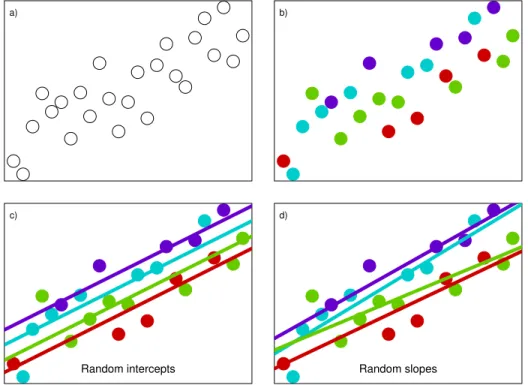
which is similar to (1) except with an additional random effects term γ1j that adjusts the slope parameter for each group (and also has distributional constraints). A simple conceptual depiction of how these two types of random effects models capture group heterogeneity is shown in Figure 1. This figure uses simulated data and can be used to compare and contrast to the M-quantile approach in Figure 2, introduced in a later section.
2.1
Random effects models for discrete data
Random effects models for continuous response variables can be extended to other data types, such as count and binary data, through the use of a generalised linear mixed model (GLMM). Letg(·) be a link function, yij be the random variable of interest, assumed to
follow a distribution from the exponential family with E(yij) = µij. The GLMM with
random intercepts is then specified by
g(µij) =x0ijβ+z
0
a) b)
c)
Random intercepts
d)
Random slopes
Figure 1: Characterising group heterogeneity through random effects models in a simple scalar y and scalar x scenario: random intercepts and/or slopes allow for group-level fitted lines. Note that the four groups in these plots are indicated by different colours. Plot a) shows the raw data; b) superimposes group membership on these data; c) shows group specific means under a linear random intercepts specification; and d) shows these means under a linear random slopes specification.
Random slopes can be added to the model in exactly the same way as in the continuous case, see (2). A GLMM is typically used to characterise group heterogeneity in count and binary data, in which it is common to assigng(·) =logit(·) andg(·) = log(·) respectively.
2.2
Small area estimators using random effects models
The most common indirect approach to SAE is through the use of random effects models (Rao and Molina, 2015). Once a random effects model is fitted using the sample data, it is relatively straightforward to calculate a predicted value of the population mean ¯yj
for small areaj, a standard objective in small area estimation. The only additional data required to compute this predicted value are the auxiliary variables for the non-sampled units in the small areas; often extracted from Census data. The usual predictor of ¯yj
under the linear mixed model is its empirical best linear unbiased predictor or EBLUP under this model, which for a linear random intercepts specification is of the form
ˆ ¯ yjEBLU P =Nj−1 X i∈sj yij + X i∈rj x0ijβˆ+z0ijγjˆ (3)
where a “hat” denotes a sample estimate (or predicted value),Nj is the population size
of small area j, sj denotes the labels of the nj sampled units in area j, and rj denotes
the labels of the Nj −nj non-sampled population units in area j. It is straightforward
to modify (3) to accommodate a random slopes model for the population data.
Since the GLMM is just a linear mixed model specification for the group-conditional mean of y, it is simple to write down a plug-in empirical predictor (EP) of the area j mean ofy under the GLMM that is almost identical to the EBLUP shown in (3),
ˆ ¯ yjEP =Nj−1 X i∈sj yij + X i∈rj g−1x0ijβˆ +z0ijγˆj . (4)
2.3
Random effects models for categorical data
Small area estimators for categorical data can be defined by extending estimators based on binary data models. In the context of a random effects approach this requires a random
effects model for a categorical response. Hartzel et al. (2001) unified multinomial logistic random effects model ideas and presented a model for hierarchical non-ordered categorical data. Molina et al. (2007) used a multinomial logistic random effects model for SAE applied to labour force status, with three categories: unemployed, employed and inactive. However the model they used had exactly the same area effect for each category, which is restrictive. A random effects structure without this constraint was described by Hartzel et al. (2001), and was utilised for SAE by Scealy (2010) and Saei and Taylor (2012). Here there is a different random effect for each response category with no restriction on the covariance structure of the effects. Generally, this more general model yields improved results compared with the constrained model suggested by Molina et al. (2007). L´ opez-Vizca´ıno et al. (2013) also applied the multinomial logistic random effects model to SAE, but with the assumption of an independent random effect for each category of the variable of interest.
3
M
-quantile models for group heterogeneity
M-quantile models (Breckling and Chambers, 1988) offer an alternative way of charac-terising group heterogeneity. TheM-quantile of order q defined by an influence function ψ for a variable Y with density function f(y) is the value mq satisfying the functional
equation
E[ψq(Y −mq)] =
Z ∞
−∞
ψq(y−mq)f(y)dy= 0. (5)
Here ψq denotes the “quantile version” of ψ, i.e. ψq(u) = 2 [(1−q)Iu≤0+qIu>0]ψ(u).
Note that when ψ(u) =sgn(u), mq is the quantile of order q for the distribution of Y.
Conversely, whenψ(u) = u,mqis the so-called “expectile” of orderqfor this distribution.
It is easy to see that whenq= 0.5 andψ(u) = sgn(u),mqis the median of the distribution
of Y, while when q = 0.5 and ψ(u) = u, mq is the mean, or expected value, of Y. For
arbitrary influence functionψ, mq is therefore the quantile generalisation of the location
parameter for Y defined by q = 0.5 and this influence function. It is well known that choosing ψ so that it is a bounded skew-symmetric function is equivalent to defining a
location parameter forY that is robust to f(y) being “outlier-prone”. Consequently the M-quantiles forf(y) defined by the same ψ will also be outlier robust.
Extending (5) to the regression case is straightforward. In the same way that the regression ofY on a vector of covariatesxis defined as the expectation ofY givenx, the regressionM-quantile of orderqforY givenxis defined as the correspondingM-quantile of the conditional distribution of Y given x. More formally, it is the function mq(x) of
xthat is the solution to the functional equation
E[ψq(Y −mq(x))|x] =
Z ∞
−∞
ψq(y−mq(x))f(y|x)dy= 0. (6)
One can specify a model for a regression M-quantile function in exactly the same way as one can specify a model for a regression function. This naturally leads to the concept of a linear regression M-quantile function, where we put mq(x) =x0βq. Note that the
regression parameter βq in this model depends on the quantile index q, which can take any value in the unit interval (0,1). Consequently this linear specification for the regres-sion M-quantiles of Y corresponds to an “ensemble” model for the complete conditional distribution ofY givenx, which makes it particularly useful for modelling the sources of heterogeneity in this conditional distribution.
Estimation of linear regression M-quantiles is usually carried out by solving an em-pirical version of (6), assuming mq(x) = x0βq. Let (yi,xi;i= 1, . . . , n) be the observed
values ofY andx, withx0i = (xi,0, . . . , xi,p) denoting thei-th row of then×(p+ 1) design
matrix X. Without loss of generality we assume xi,0 = 1 ∀i, with the other columns of
this matrix defined by the values of the explanatory variables or covariates. The estimate ˆ βq of βq then satisfies n−1 n X i=1 ψq(yi−x0iβˆq)xi =0. (7)
In practice, (7) is usually solved via iteratively reweighted least squares (IRLS), with weights
wiq =
ψq(yi−x0iβˆq)
yi−x0iβˆq
.
speci-fication, see Huber (1981). This depends on a tuning constant k and is given by ψk(u) = −k, if u≤ −k u, if −k < u < k k, if u≥k. (8)
Put ψq,k(u) = 2 [(1−q)Iu≤0+qIu>0]ψk(u). The corresponding estimate of the
Huber-type regressionM-quantile function of order q is then the function ˆmq,k(x) satisfying
n−1 n X i=1 ψq,k yi−mˆq,k(xi) σq,k xi =0. (9)
whereσq,k is a nuisance scale parameter required to ensure that ˆmq,k(x) is scale invariant,
i.e. ˆmq,k(cx) =cmˆq,k(x) whenc is a constant. It is standard to set this scale parameter
equal to the median absolute deviation (MAD) of the residuals yi −mˆq,k(xi), and to
solve (9) using IRLS as previously described. Note that under a linear specification, ˆ
mq,k(xi) =x0iβˆq,k and furthermore, survey weights are easily incorporated into the fitting
process by multiplying wiq above by the survey weight for unit i.
The Huber influence function is often favoured as it depends on a tuning constant k which provides a balance between robustness and efficiency when (9) is used to estimate the M-quantile. It also provides an intuitive middle ground between quantile regression (Koenker and Bassett, 1978) and expectile regression (Newey and Powell, 1987). In par-ticular we obtain the regression expectile whenk → ∞and the regression quantile when k →0. With any finite choice of k, the Huber influence function remains bounded, and so estimation remains robust. Furthermore, continuity ofψk(u) guarantees the existence
of a unique solution to the M-quantile functional equation for every value of q ∈ (0,1) for any variable with support over the real line. We therefore focus on this definition of ψ from now on. Throughout the remainder of the article the term “M-quantile” will im-ply a Huber M-quantile unless otherwise stated, with the M-quantile of order q defined by tuning constant k denoted by mq,k. Furthermore, we sometimes do not distinguish
between the estimated M-quantile and M-quantile itself, referring to both as the M -quantile. This is done to be concise, and only when the context makes the distinction clear.
3.1
Using
M
-quantile q-scores to characterise group
hetero-geneity
One of the earlier applications of M-quantile modelling was Kokic et al. (1997). In this article, M-quantile regression was used to calculate a performance measure which had very practical uses. The data set used for this purpose contained variables measuring productivity for Australian dairy farms. The response variable of interest was the gross returns from each farm, with five covariates: labour, land, livestock, capital and materials. The performance measureqi∗ that was calculated for thei-th farm was based on a fitted M-quantile regression model and was defined by the equation
ˆ
mq∗
i,k(xi) = yi.
These q∗i performance measures have since been referred to as M-quantile coefficients, q-values and q-scores; the latter nomenclature will be used throughout this article. These q-scores can be thought of as ordered indices between 0 and 1, where the larger (smaller) the q-score, the further “to the right (left)” the observed value yi lies on the conditional
distribution ofY given xi. When the influence function underpinning the M-quantile is
sgn(u) (so M-quantile regression is just quantile regression), this q-score is the order of that quantile of the conditional distribution whose value equalsyi. It immediately follows
thatqi∗ is uniformly distributed over (0,1) in this case. More generally, a q-score derived from fitted regression M-quantiles can be viewed as being a random variable whose distribution defines an indexing over the interval (0,1) of the conditional distribution of Y givenxi, but not necessarily one with a uniform distribution over this interval.
The q-scores defined by the conditional distribution ofY givenxon a sample can be calculated by first fitting regression M-quantiles to the sample data withq varying over a fine grid, e.g. q = 0.001, . . . ,0.999. In general, the collection of these fitted regression M-quantile models is referred to as an ensemble regressionM-quantile model, or just an ensembleM-quantile model. Such an ensemble fit allows calculation of a fitted regression M-quantile value ˆmq,k(xi) for each value ofqon the grid at each xi. The value ofqi∗ can
yi. In some instances when q is very close to 0 or 1 a solution to the estimating equation
for ˆmq,k(xi) may not exist, in which case this grid of q-values may need to be bounded
away from 0 and 1, for example, ranging from q= 0.05 to 0.95.
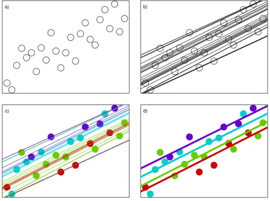
Chambers and Tzavidis (2006) exploited the fact that q-scores characterise the marginal heterogeneity of the conditional distribution of Y given x in the sample, and so can be used to do SAE based on the fit of the ensembleM-quantile model. In particular, they argued that if grouping structure underpins this heterogeneity than q-scores would tend to be more similar in groups, and could therefore be suitably “averaged” within groups or areas to obtain “group-specific” q-scores. These group-averaged indices could then be used to distinguish between the conditional distributions of Y given x in the different groups by using the component regression M-quantile fit with index equal to group q-score to characterise within group behaviour. In effect, the group q-q-score plays the same role as the group effect in a mixed effects model, but without the need to pre-specify the grouping structure. This use of q-scores for effectively modelling group heterogeneity opened up a new area of possible applications. Chambers and Tzavidis (2006) suggested that the robustness properties of the regressionM-quantile models, as well as their semi-parametric nature (no distributional assumptions) make them particularly useful with the small sample sizes found in SAE. They can also be easily adapted to multilevel es-timation problems, as was done by Tzavidis and Brown (2010) in their application to modelling pupil performance in London schools. Figure 2 provides a simple explanation of how heterogeneity is characterised usingM-quantile regression and q-scores.
In the linear case, with continuous Y, the M-quantile estimators of the small area means for this variable are simply their predicted values based on the linearM-quantile fits corresponding to the group q-scores. More precisely, let ˆq∗j be the group q-score for groupj, e.g. ˆq∗j =n−j1P
i∈sjq
∗
i if there are sampled group members, otherwise ˆq∗j = 0.5.
The M-quantile estimator for the group mean of Y is then
ˆ ¯ yjM Q =Nj−1 X i∈sj yij + X i∈rj x0ijβˆˆqj∗,k . (10)
a) b)
c) d)
Figure 2: Characterising group heterogeneity through linear regressionM-quantile mod-els: The data and set-up here are the same as those set out in Figure 1, with plot a) identical. In plot b) an ensemble M-quantile regression model with k = 1.345 is fitted where each observation has a corresponding line of exact fit and q-score equal to the index of that line. These q-scores and associated fitted regressionM-quantile lines are grouped by colour in c) and the mean q-score calculated for each group. The fitted lines shown in plot d) then characterise the four groups, i.e. they correspond to the M-quantile fits with indices equal to these group q-scores.
approach. That is, there is a parametric assumption (linearity) about the behaviour of the regression M-quantiles in the population, but no further distributional assumptions after that.
The obvious advantage of theM-quantile estimator over the EBLUP is its robustness to outliers and its lack of distributional assumptions. These are useful attributes, espe-cially under small sample sizes which can often be the case. However, the EBLUP does minimise the mean squared error (MSE) under an assumed mixed model, and so must be more efficient if this model is true (which is rather unlikely in practice). Nevertheless, Chambers and Tzavidis (2006) report results from a simulation study that shows the M-quantile small area estimator (10) performs similarly to the EBLUP (3) even when the random effects model underpinning the EBLUP is used to generate the population data.
3.2
A real data example: farm data
We illustrate the differences in the two approaches to characterising group heterogeneity for continuous variables using a real data set, rather than the simulated data presented in Figures 1 and 2. These data are from 1,652 broadacre farms spread across 29 climatic regions of Australia. The response variable of interest is the total value of the farm in dollars, with the farm area in hectares the only explanatory variable. The aim is to characterise differences in the relationship between these variables between the 29 regions. We can characterise this regional heterogeneity using either a random effects model or an M-quantile model. Two random effects models were fitted to these data; a random intercepts model and a random slopes model. Figure 3 shows the fit of these two models, as well as the fit of an ensemble-based set of regional M-quantile regression models with k = 1.345. The colourful fitted lines represent estimates of the conditional mean for each of the 29 regions. It seems clear that the random intercepts model fit fails to adequately reflect the regional heterogeneity in these data, while the random slopes model fit appears rather unstable. In contrast, theM-quantile ensemble fit seems stable and does a reasonable job of characterising regional heterogeneity in the relationship
between farm value and farm area.
4
M
-quantile models for discrete data
The definition and interpretation of M-quantiles, as well as their estimation, requires more care when applied to discrete-valued variables. To start, we note that the discretised version of the defining functional equation (6) always has a solution provided ψ is a continuous influence function, soM-quantiles specified in this way always exist. However, there are issues with developing an appropriate empirical version of (6) for this case. Chambers et al. (2014) develop M-quantile estimation for disease mapping, based on estimating the M-quantiles of the negative binomial distribution, while Tzavidis et al. (2015) consider the modelling of counts more generally, based on the M-quantiles of the Poisson distribution. Chambers et al. (2016) focus on the important case of binary data and extend these approaches to define M-quantiles for the Bernoulli distribution. In all of these developments, the M-quantile estimates are obtained by extending the Cantoni and Ronchetti (2001, referred to as CR below) quasi-likelihood approach to defining robust estimating equations for a generalised linear model. In addition to using a bounded influence function to control sample outliers, and weights to control sample leverage values, the CR approach includes an additional term in the estimating function to ensure Fisher consistency for the estimates. The CR estimating equations are of the form n X i=1 ψ(ri) 1 σ(µi) µ0i−a(β) =0, (11)
whereri = (yi−µi)/σ(µi), µi =g−1(x0iβ),µ0i =∂µi/∂β, g(·) is a link function,σ(µi) is
the standard deviation of the fitted value and
a(β) = n X i=1 E[ψ(ri)]σ−1(µi)µ0i . (12)
CR argue that addition of the consistency term a(β) is necessary to protect against inconsistent estimators of the mean, particularly for asymmetric distributions.
12 14 16 Random intercepts 12 14 16 F ar m V alue (log $) Random slopes 4 6 8 10 12 14 12 14 16
Farm Area (log ha)
M−quantile
Figure 3: Characterising regional heterogeneity in the relationship between farm value and farm area (both expressed in logs) using random effects models and M-quantile models. Each of the 29 regions, and its fitted linear model, is represented by a different
The quasi-likelihood approach of CR can be extended to estimation of regression M-quantiles for discrete data through solution of the estimating equations
n X i=1 ψq,k(ri,q,k) 1 σ(mq,k(xi)) m0q,k(xi)−a(βq,k) =0 (13) withri,q,k = (yi−mq,k(xi))/σ(mq,k(xi)),mq,k(xi) =g−1(x0iβq,k),m0q,k(xi) = ∂mq,k(xi)/∂βq,k,
σ(mq,k(xi)) is the standard deviation of the fitted value, and
a(βq,k) = n X i=1 E[ψq(riq)]σ−1(mq,k(xi))m0q,k(xi) . (14)
This a(βq,k) term ensures that mq,k(xi) is Fisher consistent for the corresponding
re-gression expectile regardless of choice of the tuning constant k. The necessity for this constraint in the discrete case is debatable, however, and there are strong arguments for omitting it from (13) on the basis that the resulting estimates have better qualitative robustness properties. Further research is ongoing in this area.
4.1
Discrete data and q-scores
We have already seen that q-scores offer a way of characterising group heterogeneity in continuous data without requiring the assumption of group-specific random effects. In particular, q-scores can be computed very simply for continuous data since their estimating function yi = mq∗
i,k(xi) will always have a solution. However this is not necessarily the case when the response is discrete such as with count and binary data. In both these cases this estimating function will not always have a solution because when yi = 0 there is no such estimated M-quantile that equals 0. This is a direct
consequence of the fact that the link function ensures that all M-quantile estimates are greater than 0. One could argue that in this case q∗i should equal 0, but then problems arise when one considers that every yi = 0 will likely have a different xi. This means
that their correspondingq∗i values be 0 regardless of their varying xi values, which is an
undesirable property.
Tzavidis et al. (2015) and Chambers et al. (2014) suggest almost identical approaches to calculating q-scores given data from a Poisson and a negative binomial distribution
respectively. The q-score q∗i for a count datum yi is obtained as the solution to mq∗ i,k(xi) = min 1−, 1 exp(x0iβq=0.5,k) , if yi = 0 yi, if yi = 1,2, . . . (15)
where >0 is a small prespecified constant. This is essentially the same definition as in the continuous case except when yi = 0, where an adjustment is made. Unfortunately,
there are two issues with this approach. Firstly, adjusting only when yi = 0, and not a
general adjustment to all values of yi, creates an artificial skewness in the q-scores, and
secondly solution of (15) requires a subjective selection of a nuisance parameter . A similar problem with defining q-scores for zero valued response data arises in the context of binary data. Chambers et al. (2016) suggest three methods to calculate q-scores in this case, but (for logistic link functions) focus on one that defines q∗i as the solution to yi∗ =x0iβq∗ i, where yi∗ = logit 1 2[mq=0.5,k(xi) +yi] . (16)
This equation corresponds to finding a halfway point between the estimated probability and the yi ∈ 0,1, from which the estimate of qi∗ can be made. This ensures that the
less probable the value ofyi given mq=0.5,k(xi), the more extreme the q-score which is an
intuitive property of the q-score.
As in the continuous response case, M-quantile approaches to SAE for discrete data use an averaged q-score within a small area to define an area level q-score, which then defines an appropriate regression M-quantile to use for predicting the average of the unobserved responses from the small area, see (10). This corresponds to a predictor of the area j mean of the discrete valued response Y of the form
ˆ ¯ yjM Q =Nj−1 X i∈sj yij + X i∈rj ˆ mqˆ∗ j,k(xij) (17) where ˆmqˆ∗ j,k(xij) = g −1(x0
ijβˆqˆ∗j,k). In the case of binary data the M-quantile estimate
ˆ
mqˆ∗j,k(xij) can be viewed as a robust estimate of the probability that yi = 1 given xij
4.2
A real data example (contd.): binary responses
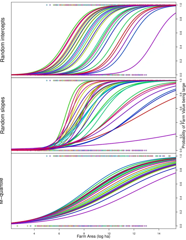
In Figure 3 we illustrated the differences in the mixed model andM-quantile approaches for characterising regional heterogeneity for continuous responses using a farm survey data set. These same farm data can also be used to display the differences between these modelling approaches in the case of a binary response. In particular, we transformed the continuous response variable corresponding to total farm value to a binary valued variable, replacing it by the indicator for whether this value is large or not. That is, we put yi = 1 when it was greater than 12×105 and set yi = 0 otherwise. Again, the
focus is on modelling the conditional distribution of this binary Y given the covariate, farm area. Two random effects models (GLMMs) were therefore fitted to these data; both based on a logistic specification with random effects on the linear scale, one with random intercepts and the other with random slopes. In addition, we fitted an M -quantile ensemble regression model withk = 1.345 based on a linear logistic specification for the M-quantile regression functions. Figure 4 compares the fit of these three models in terms of the different fitted regional models for the probability that a farm is valued highly given its size. It is again clear that the random intercepts model does not fit well, while the random slopes model exhibits considerable instability. The M-quantile model fits on the other hand seem to provide a good compromise between stability and adequately reflecting regional heterogeneity in these probabilities.
4.3
M
-quantile models for categorical data
Research is ongoing on an appropriate way of defining M-quantiles for categorical data that follow a multinomial logistic distribution. This is mainly due to the fact that with more than two categories the intuitive restriction that the sum of the M-quantiles at a particular value of xi should equal one for all values of q is inappropriate. This research
0.0 0.2 0.4 0.6 0.8 1.0 Random intercepts 0.0 0.2 0.4 0.6 0.8 1.0 Probability of F ar m V
alue being large
Random slopes 4 6 8 10 12 14 0.0 0.2 0.4 0.6 0.8 1.0
Farm Area (log ha)
M−quantile
Figure 4: Using random effects models and M-quantile models to characterise regional heterogeneity in the probability that a farm is valued highly given its size. The actual binary data are shown aty= 1 and y= 0 in each plot, with regions denoted by different
5
Conclusion
This article outlines two distinct ways in which group-level heterogeneity in data can be characterised, and then applied in SAE. The random effects approach assumes group differences are essentially due to a latent group effect. That is, group heterogeneity is a consequence of the distribution of values of these group effects. On the other hand, ensembleM-quantile regression models require no a priori specification of a group effect structure. The M-quantile approach to characterising group level heterogeneity in this case first associates an index of individual level heterogeneity with each sample response. These indices are then averaged appropriately within groups to define a group level index which can be used to identify an appropriateM-quantile model for the group within the M-quantile ensemble model. Simply put, the random effects model assumes group effects a priori, whereas the M-quantile model develops group effects a posteriori. These two approaches to characterising group effects can be utilised for a wide range of data types; including continuous, count and binary data. The preferable method will depend on the data available, with random effects models having superior theoretical properties under ideal model conditions. However M-quantile methods for characterising heterogeneity, particularly in the context of SAE, provide a useful alternative, as well as a superior approach when distributional assumptions are not met or when outliers are present.
Acknowledgements
The first author would like to acknowledge that the research reported in this article was conducted with the support of an Australian Government Research Training Program Scholarship. This scholarship was administered by the University of Wollongong on behalf of the Department of Education and Training, Australia.
References
Cantoni, E. and Ronchetti, E. (2001). Robust inference for generalized linear models.
Journal of the American Statistical Association,96, 1022-1030.
Chambers, R. and Tzavidis, N. (2006). M-quantile models for small area estimation.
Biometrika, 93, 255-268.
Chambers, R., Dreassi, E., and Salvati, N. (2014). Disease mapping via negative binomial regression M-quantiles. Statistics in Medicine, 33, 4805-4824.
Chambers, R., Salvati, N., and Tzavidis, N. (2016). Semiparametric small area estimation for binary outcomes with application to unemployment estimation for local authorities in the UK. Journal of the Royal Statistical Society: Series A (Statistics in Society),
179, 453-479.
Hartzel, J., Agresti, A., and Caffo, B. (2001). Multinomial logit random effects models.
Statistical Modelling, 1, 81-102.
Huber, P. J. (1981). Robust statistics. New York: John Wiley & Sons, Inc.
Koenker, R. and Bassett, G. (1978). Regression quantiles. Econometrica,46, 33-50. Kokic, P., Chambers, R., Breckling, J., and Beare, S. (1997). A measure of production
performance. Journal of Business & Economic Statistics,15, 445-451.
L´opez-Vizca´ıno, E., Lombard´ıa, M. J., and Morales, D. (2013). Multinomial-based small area estimation of labour force indicators. Statistical Modelling, 13, 153-178.
Molina, I., Saei, A., and Lombard´ıa, M. J. (2007). Small area estimates of labour force participation under a multinomial logit mixed model. Journal of the Royal Statistical Society: Series A (Statistics in Society), 170, 975-1000.
Newey, W. K. and Powell, J. L. (1987). Asymmetric least squares estimation and testing.
Econometrica, 55, 819-847.
Rahman, A. and Harding, A. (2016). Small Area Estimation and Microsimulation Mod-elling. Chapman and Hall/CRC Press.
Rao, J. N. K. and Molina, I. (2015). Small Area Estimation - Second Edition. John Wiley & Sons, Inc.
Saei, A. and Taylor, A. (2012). Labour force status estimates under a bivariate random components model. Journal of the Indian Society of Agricultural Statistics, 66, 187-201.
Scealy, J. (2010). Small area estimation using a multinomial logit mixed model with category specific random effects. Research Paper 1351.0.55.029, Australian Bureau of Statistics,http://www.abs.gov.au/ausstats/[email protected]/cat/1351.0.55.029. Tzavidis, N. and Brown, J. (2010). Using M-quantile models as an alternative to random
effects to model the contextual value-added of schools in London. DoQSS Working Paper No. 10-11, Institute of Education, University of London,
http://repec.ioe.ac.uk/REPEc/pdf/qsswp1011.pdf.
Tzavidis, N., Ranalli, M. G., Salvati, N., Dreassi, E., and Chambers, R. (2015). Robust small area prediction for counts. Statistical Methods in Medical Research,24, 373-395.