Clustering financial time series

University of Tartu

Faculty of Science and Technology

Institute of Mathematics and Statistics

Nshan Potikyan

Clustering Financial Time Series

Actuarial and Financial Engineering

Master’s Thesis (30 ECTS)

Supervisor: Raul Kangro, Assoc. Prof.

Clustering Financial Time Series

Nshan Potikyan

Abstract. Time series clustering is heavily based on choosing a proper dissimilarity measure between a pair of time series. We present several dissimilarity measures and use two synthetic datasets to evaluate their performance. Hierarchical clustering and network analysis methods are used to perform cluster analysis on stock price time series of 594 US-based companies in order to verify whether stock prices of companies operating within an industry have common fluctuations. The results of the thesis show that some companies within the same industry do form clusters, while others are relatively scattered.

CERCS research specialisation: P160 Statistics, operation research, program-ming, actuarial mathematics

Keywords: Time Series Analysis, Dissimilarity Measures, Cluster Analysis, Mini-mum Spanning Trees

Finantsaegridade klasterdamine

Nshan Potikyan

L¨uhikokkuv˜ote. Aegridade klasterdamise tulemused s˜oltuvad oluliselt sobiva kahe ae-grea erinevuse m˜o˜odu valikust. T¨o¨os tutvustatakse mitmeid kasutatavaid erinevusm˜o˜otusid ning hinnatakse nende abil saadavaid tulemusi kahe genereeritud andmestiku korral. Seej¨arel rakendatakse p¨ustitatud eesm¨argi jaoks sobivaimaid m˜o˜otusid koos hierarhilise klasterdamise ja v˜orgustiku anal¨u¨usi meetoditega selleks, et uurida 594 Ameerika ¨ Uhend-riikides baseeruva firma aktsiahindade aegridade puhul k¨usimust, kas t¨o¨ostusharude sis-eselt on nende aegridade k¨aitumine sarnasem kui t¨o¨ostusharude vaheliselt. Saadud tule-mused n¨aitavad, et mitmete t¨o¨ostusharude sees on sarnaste hinnamuutustega firmade r¨uhmasid, kuid on ka palju ¨ulej¨a¨anutest erineva k¨aitumisega ettev˜otteid.

CERCS teaduseriala: P160 Statistika, operatsioonanal¨u¨us, programmeerimine, finants-ja kindlustusmatemaatika

M¨arks˜onad: Aegridade Anal¨u¨us, Erinevusm˜o˜odud, Klasteranal¨u¨us, Minimaalsed Aluspuud

Contents

3 Time Series Clustering 15

3.1 Hierarchical Clustering . . . 15 3.2 Clustering Evaluation . . . 18

4 Network Analysis Methods 20

4.1 Minimum Spanning Trees . . . 20 4.2 Friedman-Rafsky test . . . 21

5 Numerical Experiments 23

5.1 Dissimilarity Selection . . . 24 5.2 Clustering Stock Prices . . . 30

6 Conclusion 36

References 38

1

Introduction

Cluster analysis or clustering is an unsupervised learning task that aims to group a set of unlabeled objects into homogeneous clusters such that the objects of the same cluster are similar to each other, and objects that belong to different clusters are dissimilar according to some pre-defined criterion. Clustering methods have been developed since the 1930s with main applications on static (non-temporal) data. In many real world applications, one needs to perform cluster analysis on time series data, which explains the growing popularity of time series clustering in recent years.

A central component of cluster analysis is the selection of a suitable dissimilarity mea-sure for a pair of data objects. In literature, there are a wide range of such meamea-sures proposed for comparing temporal data, however there is not a single dissimilarity mea-sure that suits to all types of problems. For example, a dissimilarity meamea-sure designed for detecting similar time series in shape, may not be much helpful when detecting time series with common autocorrelation structures. This means that the choice of a par-ticular dissimilarity measure should be based on the kind of similarity it captures and whether that idea of similarity is aligned with one’s clustering objective. Once the unique characteristics of the subject data are clear, one may also design an appropriate similar-ity/dissimilarity measure accordingly. Hennig and Hausdorf [14] give useful guidelines for the choice and design of dissimilarity measures.

In this work, we are interested in clustering financial time series data, such as stock prices, interest rates, exchange rates, bond yields, monthly profits or losses of a company etc. The motivation behind cluster analysis in the financial domain can be diverse, ranging from identifying groups of countries with similar dependence structures in their long-term interest rates, to detecting companies whose stock prices evolve similarly through a certain time horizon. The latter problem will be mainly discussed as a base example in this thesis, but the overall analysis can be extended to other types of financial data considering the problem-specific notion of similarity.

Portfolio analysis of large number of securities is of primary interest in financial risk management. The purpose of the analysis is to select an ensemble of securities that pro-vides both protection and opportunities to the investor, despite the future uncertainties.

One of the key strategies when building portfolios is diversification, that is investing in securities which are expected to be strongly negatively correlated in order to minimize the overall risk of the portfolio. There is a general belief that the returns on a security are more correlated with those in the same industry than those of unrelated industries [22]. Therefore, one basic strategy for diversification could be taking securities from dif-ferent industrial sectors and hence manage the risks associated with potential crises in a certain sector. While the assumption of similarly behaving returns within an industry is somewhat naive, it is worth testing whether there is any empirical evidence supporting or rejecting this line of thought. Cluster analysis with an appropriate dissimilarity measure can be used to explore this problem.

The clustering objective of this thesis is to group time series that move up and down synchronously, with possibly some short-term time delay. The idea is that an unknown random process may affect several securities at the same time, but the influence of that factor may have small latency on each of them. For example, some news may affect many agricultural companies or a natural disaster in certain region may cause solvency issues to insurance companies, leading to a downgrade in their security prices. The ideal dissimilarity measure should capture this kind of common fluctuations in the historical time series of securities.

Once the clustering objectives and the assumption of similarity/dissimilarity are fixed, the next step of the analysis should be the selection of a suitable clustering algorithm. There is not a single established distinction between many clustering methods in the liter-ature. Two popular types of methods are partitional and hierarchical clustering methods. In case of partitional clustering all observations in the data are partitioned into k dif-ferent clusters by solving an optimization problem for minimizing within-cluster distance while maximizing between-cluster distance. The number of clustersk needs to be defined in advance. Two commonly used algorithms for partitional clustering are k-means and

k-medoids that build clusters around the means (centroid) and medoids (central data point) of observations, respectively. In this work we base our attention on hierarchical clustering methods, which do not require the number of clusters to be defined in advance and build a nested hierarchy of clusters, letting the user examine potential clusters with graphical means, such as dendrograms. The idea of nested clusters is well-aligned with

our clustering objective, since two companies may belong to the same industrial sector according to a standard classification system, but we can further specify their activities within a sector, thus making a sub-sector distinction between them.

When the number of data objects (time series) gets large, dendrograms may not be much informative and minimum spanning trees (MST) may be used from graph theory in order to visualize the hierarchy of clusters, as well as to obtain clusters by removing some of its edges.

1.1

Literature Review

The pioneering work in clustering financial time series belongs to Mantegna (1999) [21], in which the author constructed a minimum spanning tree on a portfolio of stocks from S & P index, using their daily closure prices. The author investigated the resulting clusters and spotted groups of stocks operating in the same industry or sub-industry. Mantegna used a dissimilarity measure based on Pearson’s correlation coefficient on the log returns of the stock prices, which only detects synchronous similarity between time series, without considering any possible time delays in the common fluctuations.

Since the seminal paper of Mantegna, many works have followed with different method-ologies. Plerou et al. [28] introduced a clustering method based on Random Matrix Theory (RMT) with an application on stock price time series. The authors analyse the eigenvalue statistics of the empirically-measured correlation matrix against a random cor-relation matrix, in order to distinguish genuine corcor-relations from “apparent” corcor-relations that are present in random matrices. The results suggest that the eigenvalue statistics can be used to construct optimal portfolios having a stable ratio of risk to return.

Giada and Marsili [9] propose a parameter free approach for clustering based on max-imum likelihood principle. The authors test the performance of the algorithm by com-paring against standard clustering algorithms on two different data sets: time series of financial market returns and gene expression data. The results from the experiments sug-gest that some of the algorithms produce similar cluster structures whereas the outcome of standard algorithms has a much higher variability.

Tumminello et al. [31] introduce a spanning tree associated to the average linkage method of hierarchical clustering in order to remedy the stability issues of minimum

spanning trees. The authors also present bootstrap sampling method to assess link reli-ability of the generated minimum spanning tree. The reported results suggest that the introduced spanning tree is slightly better than the standard MST, based on numerical experiments conducted on 300 stocks.

Billio et al. [3] propose several dissimilarity measures based on principal-components analysis and Granger-causality tests with application on the monthly returns of hedge funds, banks, broker/dealers, and insurance companies. The authors analyze the interde-pendence of these entities for systematic risk management perspective and state that the proposed measures can identify and quantify financial crisis periods.

The remainder of this thesis is organized as follows: different dissimilarity measures are introduced in Section 2, among which there are some measures that are frequently used in practice, but are not aligned with our clustering objective. The main features of time series clustering are discussed in Section 3, with an emphases on hierarchical clustering and two popular measures for assessing the quality of obtained clusters. In Section 4, we define the minimum spanning trees in the context of community detection and formulate a permutation test to verify whether the structure of the minimum spanning tree is a result of random effects. Section 5 is devoted to numerical experiments with two phases: first, we select an appropriate dissimilarity measure, which results in better performance on synthetically generated time series and second, we use the relevant dissimilarity measure in order to form clusters with stock prices of 594 US-based companies. The results of the experiments are concluded in Section 6 with some discussion on potential future work.

The numerical experiments were conducted using R and Python programming lan-guages and all the necessary datasets, scripts can be found in this GitHub repository1_.

Two of the presented dissimilarity measures were computed using an existingTSclust [24] package in R, which provides useful tools for time series clustering.

2

Dissimilarity Measures

Time series clustering is heavily based on choosing the right dissimilarity measure among different time-series. A wide range of dissimilarity measures between time series

1

have been proposed in the literature. Here we will explore a small sample of them that are frequently used for various clustering objectives. Time series dissimilarity measures are categorized based on different criteria. In this work we will divide the set of measures into two groups: model-free and model-based approaches.

In the remainder of this section and beyond, we will use the following notations: x = (x1, . . . , xn)T and y = (y1, . . . , yn)T represent 2 time series realizations from real-valued processesX ={Xt, t∈Z}and Y ={Yt, t ∈Z}respectively. We will consider that all the series are equal in lengthn, if not stated otherwise.

Some of the dissimilarity measures are actual distance measures, that satisfy all three properties of a metric that is

1. d(x,y)≥0 ∀x,y and d(x,y) = 0 ⇐⇒ x=y (positive definite) 2. d(x,y) =d(y,x) ∀x,y(symmetric)

3. d(x,z)≤d(x,y) +d(y,z) ∀x,y,z (triangle inequality).

There are some measures that do not satisfy all these conditions, that is why we will avoid using the phrasedistance measure and instead, will usedissimilarity measure in all cases.

2.1

Model-free measures

We start with dissimilarity measures that are based on the raw time series or some features derived from them, which make no assumptions about the generating processes of the series.

2.1.1 Minkowski distance

A simple and straightforward measure of proximity between two time series of equal size is the Minkowski distance of order p ∈ _N, also known as Lp-norm distance. It is defined as follows: dLp(x,y) = Xn t=1 |xt−yt|p 1_p .

Euclidean (p = 2) and Manhattan distance (p = 1) are two well-known special cases, which are mainly used in the context of clustering. One of the drawbacks of this metric

is that it measures time-wise similarity of the series and fails to account for misalignment in time. Another drawback is that these measures are sensitive to noise, thus using them for noisy financial time series is not recommended.

2.1.2 Correlation-based

Correlation-based dissimilarity measure belongs to the family of structure-based mea-sures, and similar to Minkowski distance, it measures dissimilarity in time. Two such measures were constructed by Golay et. al [10]. They are defined by

dCOR1(x,y) = q 2(1−ρˆxy) and dCOR2(x,y) = s 1−ρˆ_xy 1 + ˆρxy β , β ≥0,

where ˆρxy is Pearson’s correlation coefficient

ˆ ρxy = n X t=1 (xt−x)(¯ yt−y)¯ s _n X t=1 (xt−x)¯ 2· s _n X t=1 (yt−y)¯ 2 ,

where ¯x and ¯y are the average values of the corresponding series. When the correlation between time series tends to −1, dCOR2(x,y) tends to infinity, while the parameter β

controls how fast the measure grows to infinity and how fast it descends towards 0. These measures detect synchronized behavior between time series and are invariant to any linear transformation. Also, when applying this measure on time series with some trend, it is useful to consider using the detrended versions of the series. One of the drawbacks of the correlation-based measures is that it is sensitive to time shifts. The latter is alleviated in the next set of dissimilarity measures, which are based on cross-correlation.

2.1.3 Cross-Correlation-based

Unlike the correlation based dissimilarity measures, cross-correlation based measures are insensitive to time shifts. Here we represent three such measures based on the sam-ple cross-correlation function (CCF), which is often used in transfer function models for

identifying the suitable lag of one time series that may be useful for predicting the future values of another time series.

The CCF of two time series xand y for time lag τ is defined as follows:

ˆ ρxy(τ) = n−τ⊕ X t=1−τ (xt−x)(¯ yt+τ −y)¯ v u u t n−τ⊕ X t=1−τ (xt−x)¯ 2 · v u u t n−τ⊕ X t=1−τ (yt+τ −y)¯ 2

for τ = 0,±1,±2, . . . . Hereτ =τ ·1{τ <0}, τ⊕ =τ ·1{τ≥0}. It should also be noted that ˆ

ρxy(τ) = ˆρyx(−τ).

In practice, the upper bound of τ is fixed and in our experiments we will consider

τmax = 10 as the maximum lag value, since in financial applications we are keen on capturing relatively short-time influences between financial time series.

One of the CCF-based dissimilarity measures was introduced by Bohte et al. [4] defined as follows: dCCF1(x,y) = v u u u u t 1−ρˆxy(0)2 τmax X τ=1 ˆ ρxy(τ)2

CCF-based dissimilarity measures were also introduced by Attila Egri et al. [6]. Here we define the measure, but with slight modification: instead of taking the maximum over the absolute values of the cross-correlations, we take the maximum value over the cross-correlations and also transform the result to make a dissimilarity measure [11].

dCCF2(x,y) =

q

2(1−max

τ ρxyˆ (τ))

We define another CCF-based dissimilarity measure, where certain weights are intro-duced for each time lag and the aggregation over the cross-correlation values takes into account the sign of theextreme cross-correlation.

dCCF3(x,y) = s 2 1−ρxyˆ (τ ∗₎ wτ∗ , whereτ∗ = argmax τ |ρˆxy(τ)·wτ| and wτ = exp − τ2 2τ2 max P τexp − τ2 2τ2 max

are the weights of each time lag cross-correlation taking value from probability density function (PDF) of normal distribution N(0, τ_max2 ). Normalization is performed to make sure that the weights sum up to one.

The choice of this particular function was made considering the shape of the PDF of normal distribution, particularly the vanishing behavior in the tails and the fact that the maximum value is in the center of mass, which is the 0 lag in our case. With this dissimilarity measure we give higher importance on the short-term time lags, assuming that the more we diverge from the 0 lag, the cross-correlations becomespurious. On the other hand, the aggregation of the cross-correlations takes into account whether the series are positively or negatively cross-correlated.

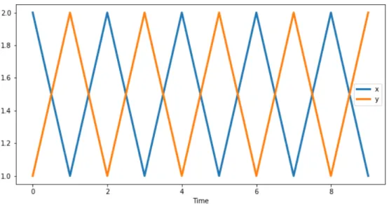
Figure 1: Time series which may be considered dissimilar if we consider the 0 lag correlation and similar if we consider 1 lag delayed cross-correlations

As an example consider these two time series of length 20

x= (2,1,2,1, . . . ,2,1)T, y= (1,2,1,2, . . . ,1,2)T

displayed in Figure 1. These time series are dissimilar if we consider their negative corre-lation in terms of the 0 lag, however they can be considered as similar if we consider the 1 lag cross-correlation. In order to resolve this contradiction, we assume that the 0 lag correlation has more weight in the final decision in comparison with the other time lags.

Also, if we take the maximum over the cross-correlations, we would get positive correla-tion between the series, this is when we need to consider the negative cross-correlacorrela-tions. On this example we have the following dissimilarity scores:

dCCF1(x,y) = 0, dCCF2(x,y) = 0, dCCF3(x,y) = 2.

2.1.4 Dynamic Time Warping

Dynamic Time Warping (DTW) is a dissimilarity measure that detects similar time series in shape, invariant of the time of occurrence of patterns. DTW aligns the two time series in a way that their difference is minimized. Unlike Minkowski and Correlation based distances, DTW can be computed on time series with different lengths.

Suppose x= [x1, . . . , xn]T and y= [y1, . . . , ym]T. In order to compute DTW distance between these time series, first we need to construct the cost matrix C ∈ _Rn×m_{, where}

Ci,j = |xi − yj|. Second, we find the warping path {(p1, q1),(p2, q2), . . . ,(pk, qk)} that minimizes

k X

i=1

Cpi,qi,

under these constraints:

• Boundary conditions: (p1, q1) = (1,1), (pk, qk) = (m, n)

• Local constraint: For any consecutive (pi, qi) and (pi+1, qi+1) it holds that (pi+1, qi+1)−

(pi, qi) ∈ {(0,1),(1,0),(1,1)}. The local constraint guarantees that the indices of the warping path are monotonically non-decreasing.

The warping distance is the cumulative sum of the elements of the cost matrix aligned with the warping path:

dDT W(x,y) = k X

i=1

Cpi,qi

It has been shown that DTW dissimilarity measure works well in applications, such as: spoken word recognition [29], gesture recognition [17], but its relevance is questionable in economic or financial applications, when we usually encounter long and noisy time series [24] . In such cases, it is more appropriate to use structure-based dissimilarity measures.

2.1.5 Autocorrelation-based

The autocorrelation-based dissimilarity measure compares the sample autocorrelation functions(ACF) of the time series. Let ˆγ_x = (ˆγx(1), . . . ,ˆγx(l))T and ˆγy = (ˆγy(1), . . . ,ˆγy(l))T be

the estimated autocorrelation vectors forxandyrespectively, for somel such that for all

i > lit holds that ˆγx(i) and ˆγy(i) are close to 0. We will follow the definition of the following

dissimilarity measure introduced by Galeano and Pena [8]

dACF(x,y) = q

(ˆγ_x−γˆ_y)T_(ˆγ

x−γˆy),

which is the Euclidean distance between the vectors of differences (ˆγ_x−γˆ_y).We can also consider partial autocorrelation functions and constructdP ACF(x,y) similarly.

Autocorrelation or partial autocorrelation-based dissimilarity measures are invariant to time shifts and also to linear transformations, for example, if we compare two time series, such that one is the linear transformation of the other, then these dissimilarity measures will consider those time series as similar. Both of these measures belong to the class of feature-based measures, that is we measure the dissimilarity between some features of the time series instead of considering the raw values. Feature-based measures are often applied to reduce the dimensionality and noise level of the original series. It can also be used to compare time series of varying lengths.

2.2

Model-based measures

Model-based dissimilarity measures typically assume that the generating processes of xand yfollow some kind of a model. Here the notion of similarity is that time series are similar if the underlying models that generated them are the same or close. The dissim-ilarity measures considered in this subsection are invariant under linear transformation and also to time-shifting, that is if two time series are similar then shifting one of the time series in time, will not change the notion of similarity.

2.2.1 Piccolo distance

Piccolo [27] introduced a distance measure based on the Euclidean distance of au-toregressive expansions of invertible ARIMA models. Therefore, suitable AR models are

fitted to each series and then the dissimilarity is measured in terms of the fitted model parameters. Let ˆΠx = (ˆπ (1) x , . . . ,πˆx(k1))T and ˆΠy = (ˆπ (1) y , . . . ,πˆ(yk2))T denote AR(k1) and AR(k2)

parameter estimations forx and y.

dP IC(x,y) = v u u t k X j=1 (πx(j)−πy(j))2,

wherek =max{k1, k2} and the smaller vector will be zero-padded.

2.2.2 Maharaj distance

Maharaj [19], [20] introduced two dissimilarity measures based on hypotheses testing to determine whether or not two time series have significantly different generating processes. The first one is given by the test statistic

dM AH(x,y) =

√

n( ˆΠx−Πˆy)TVˆ−1( ˆΠx−Πˆy),

where Πx and Πy are defined as in Piccolo’s distance and ˆV is an estimator of

V =σ_x2R−_x1(k) +σ_y2R−_y1(k),

with σ_x2 and σ_y2 denoting the variance of the white noise processes related to x and y respectively, and Rx, Ry denoting the sample covariance matrix of time series xand y.

dM AH is asymptotically χ2 distributed under the null hypothesis Πx = Πy, thus the

dissimilarity can also be measured in terms of the p-value

dM AH(p)(x,y) =P(χ2k > dM AH(x,y)).

Both of these measures are non-negative, symmetric and can be considered as dissim-ilarity measures between time series.

2.2.3 Residual-based

Baragona [2] proposed a different model-based dissimilarity measure, which considers the sample cross-correlation functions of fitted model residuals, also known asprewhitened residual series. Apart from introducing the original measure (dRCCF1), we construct two

Let ˆx and ˆy be the fitted values for x and y respectively, then this dissimilarity measure is defined by:

dRCCFi(x,y) =dCCFi(ˆx,ˆy)

for i = 1,2,3 with ˆx and ˆy being the residuals from the fitted models, for example

ˆ

x=x−xˆ.

In this thesis, the space of possible models used to fit each series is limited to autore-gressive models, possibly with first order differencing, in case the initial time series is not stationary.

3

Time Series Clustering

While forecasting is one of the most common applications of time series analysis, clustering of temporal data has gained much attention in recent years. Many general-purpose clustering algorithms have been used for time series clustering in the literature. In this section, we present commonly used hierarchical clustering method and define two indices for clustering quality evaluation.

3.1

Hierarchical Clustering

Hierarchical clustering method makes a hierarchy of clusters using divisive or agglom-erative strategies.

The divisive strategies use a top-down approach that starts with all objects as a single cluster and then splits the cluster until reaching the clusters with single objects. This strategy is rarely used in practice and there is no evidence that it is better than the agglomerative strategy, therefore we will discuss agglomerative clustering approach in more detail.

Agglomerative clustering strategy is a bottom-up approach that considers each element as an individual cluster and then gradually merges the closest pair of clusters. The pseudocode of the algorithm can be found in Algorithm 1.

The iterative merging process is of primary interest. In each iteration, a pair of clusters having the minimum distance is merged. The distance between a merged clusterCi∪Cj

Algorithm 1 Agglomerative Clustering Require: Distance matrix D∈_RN×N

1: Initialize N singleton clusters 2: while number of clusters >1do 3: Merge the closest two clusters 4: Update the distance matrix 5: end

6: return Set of nested clusters

and a clusterCk is calculated using the Lance-Williams dissimilarity update formula[25]:

d(i∪j, k) = αid(i, k) +αjd(j, k) +βd(i, j) +γ|d(i, k)−d(j, k)|, (1) whereαi, αj, β and γ are parameters that define the method for agglomerative clustering. This formula tells us that when we merge clusters Ci and Cj to form a cluster Cl, then the distance of the new clusterCl toCk is a function of distances between cluster Ck and the original clusters Ci and Cj.

Some of the well known methods for agglomerative clustering are single linkage, com-plete linkage, average linkage. Here we will describe these methods and will specify the parameter values of equation 1 for each method.

In case of the single linkage method, the parameters for Lance-Williams dissimilarity update formula areαi =αj = 0.5, β = 0 andγ =−0.5, which give us

d(i∪j, k) = 0.5d(i, k) + 0.5d(j, k)−0.5|d(i, k)−d(j, k)|=min{d(i, k), d(j, k)}.

Single linkage method can find arbitrary shaped clusters, however it is highly sensitive to noise and outliers. In case of single linkage two clusters are similar, if they have at least a pair of members, which are similar to each other, while in the case of the complete linkage linkage, the clusters are similar to each other, if all members are similar to each other.

The parameters for complete linkage method take the following values: αi = αj = 0.5, β = 0 andγ = 0.5 and plugging these values in 1 results in

Contrary to single linkage method, complete linkage is less influenced by noise and outliers, which comes with a cost of being unable to deal with arbitrary shaped clusters and bias towards breaking large clusters.

The group average linkage method is a compromise between the two extremes of single and complete linkage methods. It is derived using the following parameter values

αi = |i|

|i|+|j|, where |i| is the number of objects in cluster ci and β = γ = 0. In case of average linkage method, equation 1 takes the form

d(i∪j, k) = |i|

|i|+|j|d(i, k) + |j|

|j|+|i|d(j, k).

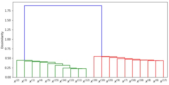
The clustering results are usually illustrated with dendrograms, like the one in Figure 2. A dendrogram provides a highly intuitive interpretation to the hierarchical clustering in a binary tree graphical format. The height of each node is proportional to the value of the inter-group dissimilarity between its two daughters. The terminal nodes, also known as leaves, represent individual observations plotted at zero height. This type of graphical representation is one of the main reasons for the popularity of hierarchical clustering methods.

Figure 2: This dendrogram is a result of applying dCCF3 dissimilarity measure with single

linkage method to cluster a set of 20 time series considered later in Section 5.

The choice of the linkage method in agglomerative clustering highly depends on the data. Each linkage method leads to a different dendrogram and one needs to be careful

with selecting the appropriate method for the data. In practice, we can expect that all these methods should provide very similar results in case of having data dissimilarities that exhibit a strong clustering tendency with well separated groups[13]. However, in case of financial time series, we rarely obtain well separated groups and the choice of the linkage method has strong influence on the outcome, as we will see in Section 5.

3.2

Clustering Evaluation

Since the task of any clustering algorithm is to detect groups in the data without prior knowledge about the ground-truth, in practice we usually do not have the true labels to compare with the results of the clustering. To alleviate this problem, usually synthetic datasets are used, such that the person who generated the dataset knows the true structure in the data. In other cases, when the true groups are not known in advance, we need to rely on internal properties of our data.

Clustering evaluation measures are typically divided into two categories:

• external index - measures the alignment between the obtained clusters and the externally supplied class (ground-truth) labels

• internal index - measures the quality of the clustering without any external informa-tion about the true labels and is based on the data distribuinforma-tion, distances between clusters or cluster centers etc.

In this section, we present one evaluation index from each category, that will be used later to verify the quality of the clusterings obtained with different dissimilarity measures. The choice of these indices was based on their popularity in time series clustering literature.

3.2.1 Similarity Index

The performance of clusterings can be tested using the cluster similarity measure, which takes into account the ground-truth labels of the time series.

Suppose G = {G1, G2, . . . Gk} is the set of k ground-truth clusters, assumed to be known, and C ={C1, C2, . . . Ck} is the set of clusters obtained by the clustering method under evaluation. The following similarity index measures the amount of agreement be-tween clusters inG and C.

Sim(G;C) = 1 n k X i=1 max 1≤j≤kSim(Gi;Cj), where Sim(Gi;Cj) = 2|Gi∩Cj| |Gi|+|Cj| .

Here| · |stands for the number of elements in the set, also known as cardinality of the set. Note that this similarity measure will return 0 if the sets of two clusterings are completely dissimilar and 1 if they are the same.

3.2.2 Silhouette Index

In cases when information about the number of clusters is not known a priori, Sil-houette index can be used to evaluate the obtained clustering. Its computation can be divided into the following steps: For time seriesxin our dataset in clusterCi, we calculate

1. its average dissimilarity with respect to all other time series in the same cluster

a(x) = 1

|Ci| −1 X

y∈Ci;y6=x

d(x,y)

2. its average dissimilarity with respect to all other time series in the nearest cluster

b(x) = min j;j6=i 1 |Cj| X y∈Cj d(x,y)

3. the Silhouette value as

s(x) =        b(x)−a(x) max{b(x), a(x)}, if |Ci|>1 0, if |Ci|= 1 .

The above measures are calculated for all time series in our dataset to obtain the final score by Sil(C) = 1 |C| |C| X i=1 1 |Ci| X x∈Ci s(x).

Silhouette index results in a score from the range [−1,1], with higher values relating to a clustering with dense and well separated clusters. It should be noted that if we try to optimize the index with respect to the number of clusters, then we will get the number of

data points (time series) as the optimal number of clusters. For this reason, in practice we try multiple values for the number of clusters and choose the one that results in maximum Silhouette index.

4

Network Analysis Methods

Networks and trees are often used to represent knowledge about a complex system. There are algorithms designed to solve the clustering problem in networks, which is com-monly referred to ascommunity detection problem. In this section, we represent minimum spanning trees from network analysis methods, which will be used to identify potential clusters. Minimum spanning trees also give topological overview of the underlying struc-ture in the data.

4.1

Minimum Spanning Trees

Minimum spanning trees were first applied for cluster detection by Zahn in 1971 [33]. We will use some definitions from graph theory in order to define minimum spanning trees.

Definition 1. A graph G is an ordered pair G= (V, E), whereV is the set of vertices or nodes and E is the set of edges or links, which are ordered (directed graph) or unordered (undirected graph) pairs of vertices.

The standard distinction between graphs is whether it is undirected or directed. In undirected graphs edges connect two vertices symmetrically, while in directed graphs the edges have certain orientations. Graphs can also have cycles (loops), which is an edge that connects a vertex to itself. In this work, we are interested in a particular type of undirected graph, also known as a tree.

Definition 2. A path in a graph is a sequence of edges joining distinct vertices.

Definition 3. A tree T is an undirected graph in which any two vertices are connected by exactly one path.

In many applications, each edge of a graph has an associated numerical value, called a weight. Usually, the edge weights are non-negative integers representing measures such as distance, similarity, dissimilarity etc. These edge weights are often referred to as the cost of the edge.

Definition 5. A minimum spanning tree (MST) is a spanning tree T such that for any other spanning tree T0 of the graph the total weight of T is less than or equal to that of

T0.

The total weight is the sum of all edge weights of the graph, representing the least expensive path passing through each vertex of the graph.

Gower et al. [12] have pointed out that the clusters resulting from applying a cut on the dendrogram obtained with a single linkage method can also be obtained by first constructing the minimum spanning tree of a graph and then cut all edges in the tree that have higher distance (dissimilarity) than the threshold applied to the single linkage dendrogram. This gives the basic intuition behind community detection using minimum spanning trees. After constructing the MST, one needs to select a threshold, such that all the edges having weights above this threshold will be considered asinconsistent edges and need to be removed in order to get the potential clusters or communities of nodes.

In literature, there are various algorithms for finding an MST. We will use Kruskal’s algorithm [16] in our experiments, which is one of the simple approaches commonly used. When there are two or more different pairs of nodes having the same dissimilarity, it is possible to obtain different MSTs with Kruskal’s algorithm. Certain optimality criteria have been introduced to select the optimal tree in such cases[5]. The pseudocode of Kruskal’s algorithm is the Algorithm 2.

4.2

Friedman-Rafsky test

After constructing the MST from our time series data, the nodes are colored according to the different categories of the time series. For example, if we have time series of stock prices, then the categories may be the sectors to which the stock-related companies belong. In this setting, we are interested whether the different categories are significantly associated with the minimum spanning tree structure.

Algorithm 2 Kruskal’s Algorithm

Require: Dissimilarity matrix D∈_RN×N 1: Initialize the tree T

2: Construct an ordered list Lfrom pairs of observations in non-decreasing order of their dissimilarities

3: while |T|<|N| −1do

4: Take the first pair (u, v) from L

5: if adding u and v toT makes no cyclesthen 6: T =T ∪ {(u, v)}

7: end

8: Remove (u, v) from L

9: end 10: return T

Suppose that we have samples of sizenandmfrom two such categoriesX = (X1, . . . , Xn) and Y = (Y1, . . . , Ym), where Xi, Yj ∈ Rd ∀i, j. Friedman and Rafsky [7] introduced an MST-based multivariate (d >1) generalization of the Wald-Wolfowitz univariate (d= 1) non-parametric two-sample test for testing the null hypothesis of FX = FY against the general alternative FX 6=FY.

In the univariate case, one needs to combine both samples in increasing order and count the number ofruns (test statistic) in that sample. A run is defined as a consecutive sequence of points from identical categories. For example, if X = (1,4,7,9) and Y = (2,3,6,10); then the combined sample will be (1,2,3,4,6,7,9,10) and the 6 runs are computed from the associated sequence of categories ”X Y Y X Y XX Y”. The idea of the test is that highly separated samples will result in a small number of runs, while highly interlaced samples will result in a large number of runs, therefore to test the hypothesis one needs to determine whether the observed number of runs is significantly large.

In order to define the multivariate analog of this test, one needs to introduce a way to order multidimensional observations. Friedman and Rafsky [7] proposed the MST-based approach, where each data point is represented as a node in the tree. After constructing the minimum spanning tree, we remove the edges connecting vertices from different

cate-gories and take the number of disjoint sub-trees as the number of runs, analogous to the univariate case.

To test whether the different categories are significantly associated with the minimum spanning tree structure or not, we use a permutation test [15] based on the ideas of Friedman-Rafsky test. Instead of the number of sub-trees, we use the number of pure edges, those that connect nodes of the same category, as our observed test statisticS0. To

assess whether the observed value is a result of randomness when the different categories have the same distribution, we randomly permute the node labels (colors) and recount the pure edges. Repeating this label shuffling procedure, we construct the null distribution of

S. We use the following biased estimator for the p-value of the permutation test in order decide whether to reject the null hypothesis

p-value = b+ 1

n+ 1, where b =Pn

i=11{Si≥S0} is the number of random permutations in which the computed

statistic has been greater or equal than the observed one andnis the number of permuta-tions. The choice of the p-value estimate should be made with caution, since if we select the unbiased estimator b

n, then the latter fails to control the type-I error of the test. [26] The idea of the test can be extended to the case when we have more than one categories for each data object (time series). For example, consider a stock network of companies operating in different countries and suppose we want to test whether, the country category effects the network structure invariant of the sector of the company. In other words, we want to find out whether there is a country effect, in case we control for the difference between sectors. The test in this case differs in terms of the permutation strategy: we permute the country labels, keeping the sector labels unchanged.

5

Numerical Experiments

In this section we compare different dissimilarity measures in order to select the one that is aligned with our objective, that is to detect structural similarity between time series invariant of time shifts. It is worth noting that when choosing the appropriate dissimilarity measure, one should not simply try all the possible dissimilarity measures

and select the one which performs the best by some predefined criteria. The choice of the measure should be based on the clustering objective and one needs to decide whether dissimilarity should be based on the overall shapes or underlying dependence structures of the time series prior to the experimental setup.

In this work we look for the dissimilarity measure that can detect structural depen-dence between time series that may be subject to some time delays. Although we can consider only those measures that are aligned with the above objective, here we also com-pare the rest of the dissimilarity measures introduced in Section 2, in order to show their drawbacks compared with the suitable measures.

Upon selection of the appropriate measure, we will use it to cluster stock prices, construct the network of stocks and will look for potential communities with minimum spanning trees.

5.1

Dissimilarity Selection

We perform a comparative analysis of the dissimilarity measures introduced in Section 2 on two synthetic datasets. Both of the datasets contain 20 time series with different degrees of similarity, designed to illustrate the limitations of the commonly used proximity measures and to test the performance of the dissimilarity measures chosen specifically for our objective.

5.1.1 Dataset 1

This dataset consists of 20 time series {x(i); i= 1, . . . ,20}of length 100 that belong to 4 classes: the first five time series belong to class C1, the next five belong to class C2

and so on. The time series in each classes are constructed as follows:

C1 ={x(i)|x (i) t =ηt+5−i+t+it} C2 ={x(i+5)|x(ti+5) =µ−ηt+5−i+t+it} C3 ={x(i+10)|x (i+10) t = 3·ηt+5−i+it},

C4 ={x(i+15)|xt(i+15)=−ηt+5−i+ 50 +it},

for t = 1, . . . ,100; i = 1, . . . ,5, where it ∼ N(0,1), η = (η1, . . . , η104) is a vector of

realizations from uniform distribution, such that η∼U(1,10), µ=_Eη= 5.5 .

The time series in each class are the shifted version of the first series of that class, for example in class C2 the series x(7),x(8),x(9),x(10) are related to x(6), so that the latter is

shifted with 1,2,3,4 lags respectively. In addition to shifting, Gaussian random noise is added to each series. The figures showing the time series in each class can be found in the Appendix.

The time series in classC1 andC2 both have an increasing linear trend, but whenever

a time series inC1 increases (decreases) with respect to the trend line, the corresponding

time series in C2 decreases (increases). In other words, the time series in C2 are the

re-flected (with respect to the trend line) versions of the series inC1. The above observations

are true for the time series in C3 and C4, with the only difference being that these series

have no trend, so their fluctuations are with respect to a horizontal line.

ClassC3 andC4 consist of time series that have no trend, but they increase or decrease

synchronously with the corresponding time series from classC1 and C2 respectively, with

some differences in the magnitudes of those fluctuations. According to our notion of similarity, the time series should be considered as similar if their fluctuations with respect to the trend lines have the same direction possibly with short-term time delays.

The synthetic time series are designed such that the ones in C1 and C3 are similar to

each other and should be considered as one cluster, while those that belong toC2 and C4

form the other cluster of similar time series. In other words, there are two ground-truth clusters and ideally the perfect dissimilarity measure should capture this pattern. Here we should note that if the similarity criterion was the shapes of the time series, then we would consider the series in C1 and C2 more similar to each other and because our

objective is to find the similar time series in terms of underlying structural dependence, then this is not the case.

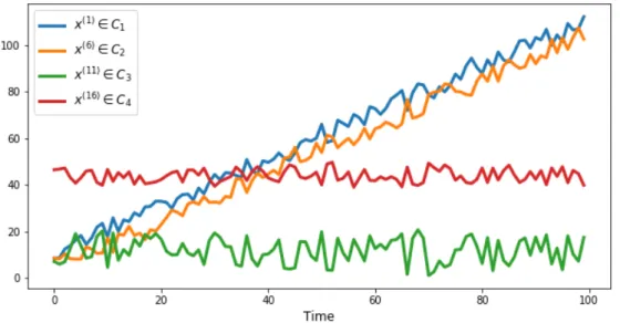
Figure 3 shows the first time series from each class and visually gives an overall idea how the time series in each group are related to each other.

dis-Figure 3: The first time series in each class.

similarity measures. The cluster labels are obtained by cutting the respective dendro-grams, such that we are left with two clusters, as in the ground-truth cluster set. Cluster-ing was performed usCluster-ing sCluster-ingle, complete and average linkage methods. The results of the clusterings were not significantly different for each linkage type on both of the synthetic datasets, hence we present the clustering results obtained with the single linkage method, because of its relation to minimum spanning trees. On the other hand, we expect the ideal dissimilarity measure to discriminate between the designed classes independent from the choice of the linkage method.

When using correlation-based measures the first order differences of the series are compared against each other, because using correlation-based measures on time series with trends is not meaningful. Also, the time series have been transformed into [0,1] range before using Euclidean distance and Dynamic Time Warping measures, which are sensitive to scaling. Here we have used the MinMax scaling technique

x0 = x−min(x) max(x)−min(x).

Table 1 contains the clustering evaluation results in terms of the similarity index. One can see that three out of four cross-correlation-based measures perfectly captured the similarities in the designed time series, thus resulted in maximum similarity index.

with-Measure Dataset 1 Dataset 2 dL2 0.5 0.36 dCOR1 0.6 0.33 dCOR2 0.6 0.33 dCCF1 0.45 1 dCCF2 1 1 dCCF3 1 1 dDT W 0.5 0.38 dACF 0.5 0.32 dP ACF 0.43 0.36 dP IC 0.5 0.38 dM AH 0.5 0.38 dRCCF1 0.5 1 dRCCF2 1 1 dRCCF3 1 0.72

Table 1: Comparison of dissimilarity measures obtained on clustering results for the two syn-thetic datasets usingSim(G;C) measure.

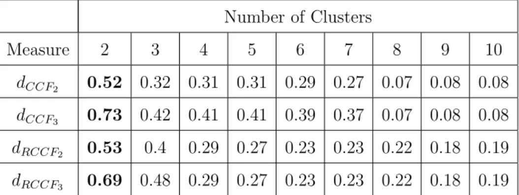
out using the knowledge about the number of true clusters in the data. Silhouette index is used to decide the optimal value for the number of clusters and the results are summarized in Table 2. Number of Clusters Measure 2 3 4 5 6 7 8 9 10 dCCF2 0.52 0.32 0.31 0.31 0.29 0.27 0.07 0.08 0.08 dCCF3 0.73 0.42 0.41 0.41 0.39 0.37 0.07 0.08 0.08 dRCCF2 0.53 0.4 0.29 0.27 0.23 0.23 0.22 0.18 0.19 dRCCF3 0.69 0.48 0.29 0.27 0.23 0.23 0.22 0.18 0.19

Table 2: Silhouette index for each clustering obtained on Dataset 1 with the competitive dissimilarity measures based onSim(G;C) index

We can see that the Silhouette index suggests that two clusters should be formed on this data invariant of the four dissimilarity measures.

The time series in this dataset shared common simple structures and it is highly improbable to encounter such time series in practice. For example, time series in each class had the same overall trend, furthermore all the time series were affected by the same random process but in opposite ways. To make things more realistic, we construct another dataset and do similar analysis on this dataset.

5.1.2 Dataset 2

Similar to Dataset 1, this dataset is also composed of 20 time series that come from 4 initial classes {Ci; i = 1,2,3,4}. The main differences with respect to the Dataset 1 are the following:

• the 5 time series in each class have different trends, but they share the same random effect (fluctuations with respect to the trend lines) with short-term time delays

• each class was generated with different random effects.

The time series in class C1 are generated with the following formulas and the type of

trend is specified in the parenthesis:

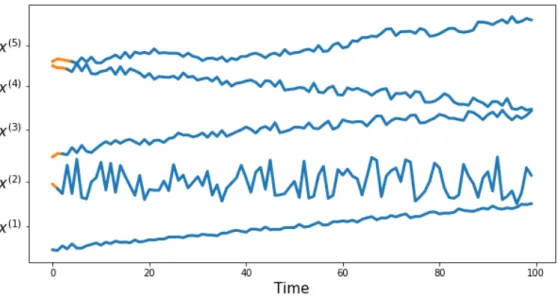
x(1)_t =ηt+4+t+1t (increasing linear) x(2)_t = 3ηt+3+2t (no trend) x(3)_t =ηt+2+ 5 √ t+3t (increasing square-root) x(4)_t = 100 + 3ηt+1−t+4t (decreasing linear) x(5)_t = 30 + 2ηt+zt+1+5t (ARIMA trend)

for t = 1, . . . ,100; where it ∼ N(0,1), η = (η1, . . . , η104) is a vector of realizations

from uniform distribution, such that η ∼ U(1,10) and zt+1 = zt+ 0.85(zt−zt−1) +0t, in other words zt+1 (with z0 = 0) are realizations of ARIMA(1,1,0) model with 0.85

autoregressive coefficient and 0_t ∼ N(0,1). Figure 4 shows the respective time series in

C1.

The rest of the time series of the other classes are generated similarly, but with different realizations of η and with different ARIMA trend in the fifth time series. The figures of the other time series can be found in the Appendix.

Figure 4: The time series inC1Class (Dataset 2). The blue parts of the series show the shifted parts of the random effect.

Each class consists of time series that should be considered similar to each other, despite having different trends. Ultimately, the clustering algorithm should group the time series from Dataset 2 into 4 clusters formed from the initial classes.

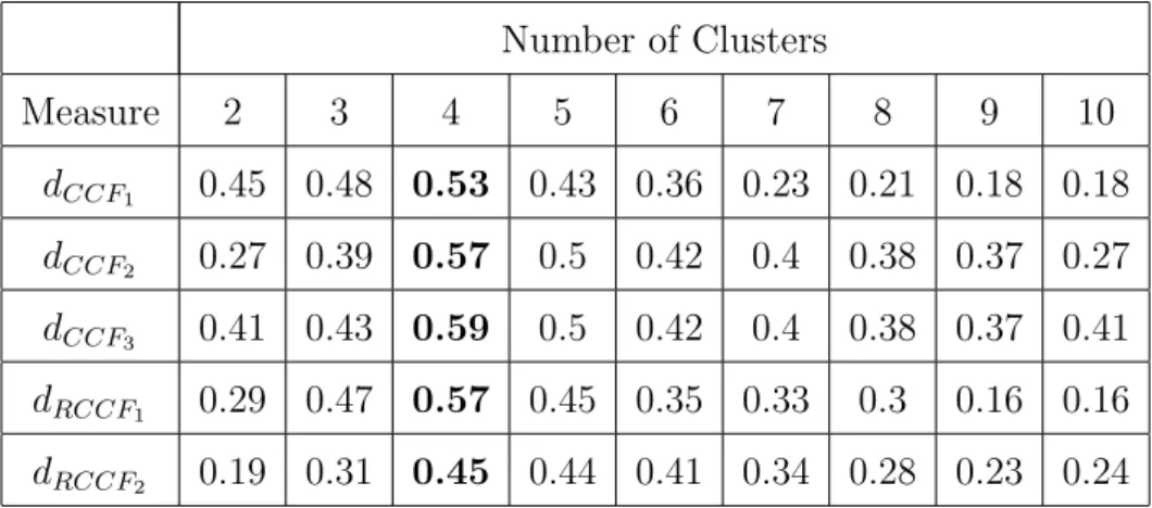
Table 1 contains the clustering evaluations of different dissimilarity measures in terms of the similarity index Sim(G;C). One can see that for this dataset all the cross-correlation-based dissimilarity measures were able to achieve perfect clusterings, when cutting the respective dendrograms at a level that results in 4 clusters. Here we explicitly used our prior knowledge about the number of ground-truth clusters in the dataset.

As in the case of Dataset 1, we also consider different number of clusters, in order to see whether we achieve better clusterings with any other number of clusters. The outcomes of Silhouette index are summarized in Table 3. We can see that all the candidate dissimilarity measures obtain the maximum value in case of 4 clusters, withdCCF3 being insignificantly

better than the rest.

Concluding the results obtained on both of the synthetic datasets, we see that clus-tering with the cross-correlation-based measures results in significantly better clusclus-terings than using the rest of the dissimilarity measures. The latter is true in case of our notion of similarity, since the synthetic datasets were generated to check the discriminating power

Number of Clusters Measure 2 3 4 5 6 7 8 9 10 dCCF1 0.45 0.48 0.53 0.43 0.36 0.23 0.21 0.18 0.18 dCCF2 0.27 0.39 0.57 0.5 0.42 0.4 0.38 0.37 0.27 dCCF3 0.41 0.43 0.59 0.5 0.42 0.4 0.38 0.37 0.41 dRCCF1 0.29 0.47 0.57 0.45 0.35 0.33 0.3 0.16 0.16 dRCCF2 0.19 0.31 0.45 0.44 0.41 0.34 0.28 0.23 0.24

Table 3: Silhouette index for each clustering obtained on Dataset 2 with the competitive dissimilarity measures based onSim(G;C) index

of the different measures. We can also see that usingdCCF2, dCCF3 and dRCCF2 measures

the clusters were perfectly aligned with the ground-truth labels. We will use dCCF2 and

dCCF3 measures in order to construct the minimum spanning trees in the next subsection,

since they are based on the raw time series and their computations do not require fitting models to each time series as in the case ofdRCCF2.

5.2

Clustering Stock Prices

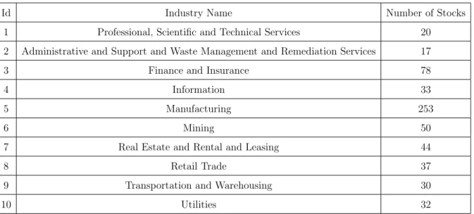
In this part of the numerical experiments, we use daily closing prices2 of 594 US-based companies of the whole period of 2019. Alongside with the time series, we have also obtained the industry information for each company. The industry names are coded by the North American Industry Classification System3 _{(NAISC). In general, each company}

may provide products or services in different industries, however the base operations of the selected companies in our dataset are limited to the specified sectors. Table 4 contains the distribution of the stock price time series per each industry.

Although there is an imbalance towards the stocks of companies operating in the Manufacturing industry, we did not down-sample the time series in this class, since in general, the distribution of companies among different industries may not be close to being uniform.

The initial step of our experiment is to construct the dissimilarity matrices of the

2

https://finance.yahoo.com

Id Industry Name Number of Stocks

1 Professional, Scientific and Technical Services 20

2 Administrative and Support and Waste Management and Remediation Services 17

3 Finance and Insurance 78

4 Information 33

5 Manufacturing 253

6 Mining 50

7 Real Estate and Rental and Leasing 44

8 Retail Trade 37

9 Transportation and Warehousing 30

10 Utilities 32

Table 4: Distribution of the observed stocks per sector using the NAISC codes.

time series using the two pre-selected dissimilarity measures dCCF2 and dCCF3. Figure 5

shows the histogram of pairwise dissimilarities of the time series for each of the dissimi-larity measure. We can see that using dCCF2 results in a truncated histogram, where the

dissimilarities between certain time series is not captured. It should be noted that our ultimate goal is not to show the potential strengths and weaknesses of these dissimilarity measures, but rather we want to explore whether the stock prices of companies operating in the same industry have co-movements that can be detected using the cross-correlation-based measures.

When constructing the minimum spanning trees based on the resulting dissimilarity matrices, we noticed that both of these measures result in the same MST. The reason is that the dCCF3 measure gives the same results as dCCF2, in cases when the series are

positively cross-correlated and the cross-correlations for the short-term lags are not signif-icantly larger than the rest of the cross-correlations after applying the lag weights. Hence, the identical minimum spanning trees are obtained on such kind of time series. On the other hand, since the dissimilarities obtained with thedCCF2 measure are bounded above

by 1.4 (see Figure 5), it is clear that the maximum weight of an edge in the MST is at most 1.4. In order to remove inconsistent edges from the tree, we consider two values for the threshold 1 and 0.8. The choice of this arbitrary thresholds was made by considering the histograms of the dissimilarity values.

Figure 5: The pairwise dissimilarities between the stock prices using dCCF2 anddCCF3

dissim-ilarity measures.

Figure 6: Network of the stocks when using threshold 1 on dissimilarities. The sector ids correspond to the ones displayed in Table 4

Figure 6 shows the MST after removing the edges having weights (dissimilarities) above 1. The layout of the tree is modified for visual purposes with the visualization tool. We can see potential groupings by visually inspecting the network. For example, most of the manufacturing companies are concentrated in the middle-left part of the network, or the ones that belong to the Mining industry are mostly clustered together in the lower part. Also, in the upper right corner of the network we can spot the disconnected nodes.

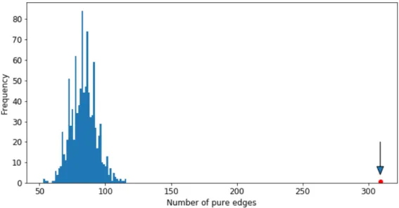
Figure 7: The histogram shows the permutation results on the first network and the arrow points to the number of observed pure edges marked with red

There are 373 total edges left in the network and 309 of those are pure edges that connect companies from the same industry. In order to test whether the observed value for the pure edges has occurred due to chance, we apply the permutation test based on the Friedman-Rafsky test by shuffling the node categories (colors) of the network for 10000 times and recalculate the number of pure edges after each permutation in order to estimate the null distribution of the pure edges. The results of the permutations are displayed in Figure 7 in terms of a histogram. We can see that the observed value for the pure edges is significantly far from the permutation results, thus there is sufficient evidence for concluding that the structure of MST is not a result of random effects.

Next, we apply the second threshold on the network edges by removing the ones above 0.8 threshold. This results in a network, where only 116 edges are left, from which 109 are

pure. The network is displayed in Figure 8. One can see there are isolated communities of companies operating in industries, such asUtility,Mining,Real Estate and Rental and Leasing. Also, we can see that there are companies from Manufacturing and Finance and Insurance industries that have similar stock price fluctuations.

The results of the permutation test applied on this network also supports the hypoth-esis that the structure in the network is related to the company industries. The histogram of the permutation results can be found in the Appendix.

Figure 8: Network of the stocks when using threshold 0.8 on dissimilarities. The sector ids correspond to the ones displayed in Table 4

Minimum spanning trees enable us to visualize the resulting clusters similar to den-drograms in case of hierarchical clustering. As in the case the synthetic datasets, we use hierarchical clustering to obtain potential groups of time series with similar fluctuations with respect to their trend lines. We use both of the dissimilarity measuresdCCF2, dCCF3

and try different linkage methods to cluster the time series into 10 clusters in order to see how much those resulting clusters are aligned with the sectors of the companies.

Dissimilarity Measure Linkage Type dCCF2 dCCF3

Single 0.08 0.08

Complete 0.33 0.26

Average 0.15 0.14

Table 5: Comparison of the similarity index Sim(G;C) on clustering results obtained with different linkage methods and dissimilarity measures

and the sector types of the companies. Since the minimum spanning trees were identical for both of this measures, not surprisingly the single linkage method used with both measures gives the same results. We can also see that using complete linkage method we obtain clusters that are more aligned with the true sector types of the companies, with

dCCF2 measure having slightly higher similarity index than with dCCF3.

Figure 9: Histogram of the 10 clusters obtained withdCCF2 measure using the complete linkage

method. The proportions of each sector are displayed on each bar. The sector ids correspond to the ones displayed in Table 4

investigated in Figure 9. We can see that the majority of the stocks in cluster 1 belong to Manufacturing, then Finance and Insurance industries or the cluster 2 and 3 are dominated by stocks from Utilities and Mining sectors respectively. A similar graph for the complete linkage method with dCCF3 measure can be found in the Appendix.

The results of the clusterings show that there is some alignment between the clusters and the sector types, but in general one cannot simply state that stock time series that have similar fluctuations are of companies operating in the same industry. In practice, stock prices of different companies operating in different industries may be affected by the same random factor.

6

Conclusion

In this thesis, we presented an end-to-end process for clustering financial time series. A central component in this process is the choice of the dissimilarity measure between a pair of time series. First, we represented various dissimilarity measures designed for different objectives and later showed that using irrelevant measures results in significantly poor clusterings. This means that the choice of the dissimilarity measure should be made with care by making sure that the observed measure represents the desired concept of similarity or dissimilarity between the time series under study.

In case of our notion of similarity, clusterings with the cross-correlation-based dis-similarity measures significantly outperformed the rest of the measures on synthetically generated datasets and the clustering of stock prices was performed using two of those measures.

Minimum spanning trees were used to view the topological ordering of the stocks. In particular, two trees were constructed by applying 1 and 0.8 thresholds on the edges of the initial MST. We used a permutation test to verify that the structure of the obtained minimum spanning trees is significantly different from what would be in case of random labelling the tree nodes.

Finally, hierarchical clustering was performed using single, complete and average link-age methods. The results showed that complete linklink-age method provides clusterings that are better aligned with the industrial sector information of each stock. Some of the

ob-tained clusters were dominated by stocks from a certain sector, while the others were a random mixture of different stocks. In our analysis we also encountered cases, when a cluster is mainly formed with stocks from two sectors. This can be explained in various ways: for example it is possible that the companies from different sectors are partners with the same third party, for example government and their co-movements are related to this factor. Another possible reason can be that the companies from different industries are collaborating together. Thus, having more information about the companies can help to further partition the high-level clusters.

It would also be interesting to see whether the observed clusters persist through time, since the dynamics of a time series may become more similar to time series of other clusters as we change the observed time horizon.

References

[1] Agrawal, R., C. Faloutsos, and A. N. Swami (1993). ”Efficient similarity search in sequence databases”. In Proceedings of the 4th International Conference on Foundations of Data Organi-zation and Algorithms, FODO ’93, London, UK, UK, pp. 69–84. Springer-Verlag.

[2] Baragona, R. (2001). ”A simulation study on clustering time series with meta-heuristic methods”, Quad. Stat. 3, 1–26.

[3] Billio, M., M. Getmansky, A. W. Lo, L. Pelizzon (2012). Econometric measures of connectedness and systemic risk in the finance and insurance sectors, Journal of Financial Economics 104, 535–559. [4] Bohte, Z.D., Cepar, D., Kosmelu, K. (1980). ”Clustering of time series”, COMPSTAT 80,

Physica-Verlag, 587-593.

[5] Djauhari, M. A., S. L. Gan (2015). ”Optimality problem of network topology in stocks market analysis”, Physica A 419, 108–114.

[6] Egri, A., I. Horv´ath, F. Kov´acs, R. Molontay and K. Varga (2017). ”Cross-correlation based clus-tering and dimension reduction of multivariate time series,” IEEE 21st International Conference on Intelligent Engineering Systems (INES), Larnaca, pp. 000241-000246.

[7] Friedman, Jerome H, and Lawrence C Rafsky (1979). ”Multivariate Generalizations of the Wald-Wolfowitz and Smirnov Two-Sample Tests.” The Annals of Statistics, 697–717.

[8] Galeano P, Pena D (2000). ”Multivariate Analysis in Vector Time Series.” Resenhas do Instituto de Matemtatica e Estatistica da Universidade de Sao Paulo, 4(4), 383-403.

[9] Giada, L., M. Marsili (2002). ”Algorithms of maximum likelihood data clustering with applications”, Physica A: Statistical Mechanics and its Applications 315, 650–664.

[10] Golay, X. S. Kollias, G. Stoll, D. Meier, A. Valavanis, P. Boesiger (1998). ”A new correlation-based fuzzy logic clustering algorithm for fMRI”, Mag. Resonance Med. 40, 249–260.

[11] Gower, J. C. (1966). Biometrika 53, 325

[12] Gower, J. C. and G. J. S. Ross (1969). ”Minimum Spanning Trees and Single Linkage Cluster Analysis” J. R. Stat. Soc.: Ser. C 18, 54–64

[13] Hastie, T., Tibshirani, R., & Friedman, J. H. (2009). ”The elements of statistical learning: data mining, inference, and prediction.” 2nd ed. New York: Springer, pp 520-524.

[14] Hennig C., Hausdorf B. (2006) ”Design of Dissimilarity Measures: A New Dissimilarity Between Species Distribution Areas”. In: Batagelj V., Bock HH., Ferligoj A., ˇZiberna A. (eds) Data Science and Classification. Studies in Classification, Data Analysis, and Knowledge Organization. Springer, Berlin, Heidelberg

[15] Holmes, S., W. Huber. (2018). ”Modern Statistics for Modern Biology”, Cambridge University Press, pp. 272-274

[16] Kruskal, J. B. (1956). ”On the shortest spanning subtree of a graph and a travelling salesman problem”. Proc. Amer. Math. Soc., 7, 48-50.

[17] Kuzmanic, A., Zanchi, V. (2007). ”Hand shape classification using DTW and LCSS as similarity measures for vision-based gesture recognition system”. In Proceedings of the International Confer-ence on “Computer as a Tool”, pp. 264–269

[18] Liao TW (2005). ”Clustering of Time Series Data : A Survey.” Pattern Recognition, 38(11),1857-1874.

[19] Maharaj EA (1996).”A Significance Test for Classifying ARMA Models.” Journal of Statistical Computation and Simulation, 54(4), 305-331.

[20] Maharaj EA (2000). ”Clusters of Time Series.” Journal of Classification, 17(2), 297-314. [21] Mantegna, R.N. (1999). “Hierarchical Structure in Financial Markets”, Eur Phys J, B11, 193, [22] Markowitz, H. (1959). ”Portfolio Selection: Efficient Diversification of Investments”. Yale University

Press

[23] Marti, G., Nielsen, F., Bi´nkowski, M., & Donnat, P. (2017). ”A review of two decades of correlations, hierarchies, networks and clustering in financial markets”. arXiv: Statistical Finance.

[24] Montero, P., & Vilar, J. (2014). ”TSclust: An R Package for Time Series Clustering”. Journal of Statistical Software, 62(1), 1 - 43.

[25] Murtagh, F. and P. Contreras (2011). Methods of hierarchical clustering. CoRR abs/1105.0121, 61–64.

[26] Phipson, B., and Smyth, G. K. (2010). ”Permutation p-values should never be zero: calculating exact p-values when permutations are randomly drawn.” Stat. Appl. Genet. Molec. Biol. Volume 9, Issue 1, Article 39

[27] Piccolo D. (1990). ”A Distance Measure for Classifying ARIMA Models.” Journal of Time Series Analysis, 11(2), 153-164.

[28] Plerou, V., P. Gopikrishnan, B. Rosenow, L. N. Amaral, H. E. Stanley (2000). A random matrix theory approach to financial cross-correlations, Physica A: Statistical Mechanics and its Applications 287, 374–382.

[29] Sakoe, H., Chiba, S. (1978). ”Dynamic programming algorithm optimization for spoken word recog-nition”. IEEE Trans. Acoust. Speech Signal Process, 26, 43–49.

[30] Rousseeuw, P. (1987). ”Silhouettes: a graphical aid to the interpretation and validation of cluster analysis.” J. Comput. Appl. Math., volume 20, no. 1, pp. 53–65

[31] Tumminello, M., C. Coronnello, F. Lillo, S. Micciche, R. N. Mantegna (2007). ”Spanning trees and bootstrap reliability estimation in correlation-based networks”. International Journal of Bifurcation and Chaos 17, 2319–2329.

[32] Wald, A. and J. Wolfowitz (1940), ”On a test whether two samples are from the same distribution”, Ann. Math. Statist., Vol. 11, 147–162.

[33] Zahn C. T. (1971). ”Graph-theoretical methods for detecting and describing gestalt clusters,” IEEE Transactions on Computers, vol. 20, no. 1, pp. 68–86

Appendix

Figure 10: Time series of classC1 in Dataset 1

Figure 12: Time series of classC3 in Dataset 1

Figure 14: Time series of classC1 in Dataset 2

Figure 16: Time series of classC3 in Dataset 2

Figure 18: The results of the permutations in case of the network with threshold 0.8 applied on edges

Figure 19: Histogram of the 10 clusters obtained with dCCF3 measure using the complete

linkage method. The proportions of each sector are displayed on each bar. The sector ids correspond to the ones displayed in Table 4

Non-exclusive licence to reproduce thesis and make thesis public

I, Nshan Potikyan,

1. herewith grant the University of Tartu a free permit (non-exclusive licence) to reproduce, for the purpose of preservation, including for adding to the DSpace digital archives until the expiry of the term of copyright, ”Clustering Financial Time Series”, supervised by Assoc. Prof. Raul Kangro.

2. I grant the University of Tartu a permit to make the work specified in p. 1 available to the public via the web environment of the University of Tartu, including via the DSpace digital archives, under the Creative Commons licence CC BY NC ND 3.0, which allows, by giving appropriate credit to the author, to reproduce, distribute the work and communicate it to the public, and prohibits the creation of derivative works and any commercial use of the work until the expiry of the term of copyright. 3. I am aware of the fact that the author retains the rights specified in p. 1 and 2. 4. I certify that granting the non-exclusive licence does not infringe other persons’

intellectual property rights or rights arising from the personal data protection leg-islation.

Nshan Potikyan 26/05/2020