Simulation Modelling Practice and Theory

(1)

Adaptive routing in wormhole-switched necklace-cubes: Analytical

modelling and performance comparison

Sina Meraji, Hamid Sarbazi-Azad

*

Department of Computer Engineering, Sharif University of Technology, Tehran, Iran School of Computer Science, Institute for Research in Fundamental Sciences, Tehran, Iran

a r t i c l e

i n f o

Article history:

Available online 14 June 2009

Keywords: Interconnecting network Hypercube Necklace hypercube Adaptive routing Wormhole switching Performance evaluation Analytical modelling

a b s t r a c t

The necklace hypercube has recently been introduced as an attractive alternative to the well-known hypercube. Previous research on this network topology has mainly focused on topological properties, VLSI and algorithmic aspects of this network. Several analytical models have been proposed in the literature for different interconnection networks, as the most cost-effective tools to evaluate the performance merits of such systems. This paper proposes an analytical performance model to predict message latency in wormhole-switched necklace hypercube interconnection networks with fully adaptive routing. The analysis focuses on a fully adaptive routing algorithm which has been shown to be the most effective for necklace hypercube networks. The results obtained from simulation experiments conﬁrm that the proposed model exhibits a good accuracy under different operating conditions.

1. Introduction

A large number of interconnection networks have been proposed and studied for highly parallel distributed-memory

multicomputers[6]. Among them the hypercube has been one of the most famous ones which has many desirable properties

such as logarithmic diameter and fault-tolerance. It is not, however, scalable from hardware cost point of view, i.e. when adding some few nodes to it, we have to duplicate the network size to reach the next speciﬁed network size. Other drawback

with hypercubes was reported by Patel et al.[16]when considering VLSI layout. They showed that the minimum number of

tracks for VLSI layout of ann-cube (n-dimensional hypercube) using a one-dimensional implementation has an order of

net-work size. Their investigation revealed that for an example netnet-work of 1k processors (a 10-cube), at least 687 tracks are required for VLSI implementation.

The necklace hypercube, introduced in[19], is a new interconnection network based on the hypercube network. While

preserving most of properties of the hypercube, it has some other desirable properties such as hardware scalability and

efﬁ-cient VLSI layout that make it more attractive than an equivalent hypercube network[19].

There are three main approaches for performance evaluation of interconnection networks. The ﬁrst one is monitoring the behaviour of the actual system; it can capture the effects of low-level design choices, but restricts experimentation with dif-ferent router policies since it can be prohibitively expensive and time-consuming to change these features. Simulation is the second approach for performance evaluation of interconnection network. We may implement different routing algorithms, different switching methods, and different interconnection topologies with simulation environments, but simulation is time consuming especially when we study large networks. The last way is to using mathematical approaches for performance analysis of interconnection networks. Mathematical models are cost-effective and versatile tools for evaluating system

* Corresponding author.

E-mail address:[email protected](H. Sarbazi-Azad).

Contents lists available atScienceDirect

Simulation Modelling Practice and Theory

j o u r n a l h o m e p a g e : w w w . e l s e v i e r . c o m / l o c a t e / s i m p a t

(2)

performance under different design alternatives. The signiﬁcant advantage of analytical models over simulation is that they can be used to obtain performance results for large systems and their behaviour under network conﬁgurations and working conditions which may not be feasible to study using simulation on conventional computers due to the excessive computa-tion and memory demands.

Several researchers have recently proposed analytical models of popular interconnection networks, e.g. k-ary n-cubes,

tori, hypercubes, and meshes[1–5,7,8,14,17]. The most difﬁcult part in developing any analytical model of adaptive routing

is the computation of the probability of message blocking at a given router due to the number of combinations that have to be considered when enumerating the number of paths that a message may have used to reach its current position in the network. Almost all studies on necklace hypercube interconnection networks focus on topological properties and algorith-mic issues. There has been hardly any study on performance evaluation of such networks and no analytical model proposed for necklace hypercubes. In this paper, we discuss performance issues of necklace hypercube graphs by introducing a rea-sonably accurate mathematical model to predict the average message latency in wormhole necklace hypercubes using a

high-performance routing algorithm proposed in[11,12]. An early version of this paper appeared in[13].

The rest of this paper is organized as follows. In Section2, the structure of the necklace hyeprcube is described. In Section

3, adaptive wormhole routing in the necklace hypercube is discussed. Section4proposes a mathematical performance model

for adaptive routing in wormhole necklace hypercube. Validation of the proposed performance model is realized in Section5

using results obtained from simulation experiments. In Section6, using the proposed analytical the performance of necklace

hypercubes is compared to equivalent hypercube under different implementation constraints. Finally, Section7concludes

the paper.

2. The necklace hypercube graph

The necklace hypercube is an undirected graph that is based on a hypercube by appending a necklace of processors (or nodes, interchangeably) to each edge. That is, besides connecting adjacent nodes (according to the base hypercube topology),

we connecti-th dimension neighbors by an array of nodes, as a necklace. The necklace length may be ﬁxed or variable for

different edge necklaces. In the former, there are ﬁxed number of nodes between each two adjacent neighbors on a necklace.

The network is calledregular necklace hypercube, and can be deﬁned asðn;kÞ-RNH, wherenis the number of dimensions and

kis the necklace size. With ﬁxed length necklaces, however, scaling up the network is limited to speciﬁed network sizes

indi-cated bynandkas 2n1

ðnkþ2Þ. In the latter form of necklace hypercubes, named asirregular necklace hypercube, each

neck-lace associated to channel iin the base hypercube, containskinodes. Hence, the network can be deﬁned by a vector of

n2n1

elements, i.e.k¼ ðk1;k2;. . .;kn2n1Þ. Such a network, denoted asðk1;k2;. . .;kn2n1Þ INH, has excellent scalability with

theoretically no limitations to scale. The network size for aðk1;k2;. . .;kn2n1Þ INHis given as 2nþPn2

n1

i¼1 ki. The second factor

in network size expression (the sigma part) implies the scalability property as we can have any desirable value for

ki;16_i6_n2n1_;_{in the network.}

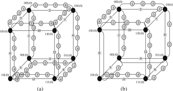
Fig. 1a and b shows some examples of regular and irregular necklace hypercubes. Dark nodes are the nodes in the base hypercube and grey nodes are the necklace nodes. The index of each necklace node in its necklace is shown inside the node.

Edge number of each edge in the base hypercube is shown inside a grey rectangle which is based on theith dimension edge

of smaller base vertex. Let us now give a more formal deﬁnition of the necklace hypercube.

1 2 1 2 3 4 000 (0) 1 2 1 2 3 4 1 2 3 1 2 3 4 1 2 3 1 2 3 4 1 2 3 1 2 010 (0) 100 (0) 001(0) 011(0) 110 (0) 101(0) 111(0) 1 2 3 4 5 6 7 8 9 10 12 11 1 2 3 4 1 2 3 4 000 (0) 1 2 3 4 1 2 3 4 1 2 3 4 1 2 3 4 1 2 3 4 1 2 3 4 1 2 3 4 1 2 3 4 1 2 3 4 1 2 3 4 010 (0) 100 (0) 001(0) 011(0) 110 (0) 101(0) 111(0) 1 2 3 4 5 6 7 8 9 10 12 11

(a)

(b)

(3)

Deﬁnition 1. A necklace hypercube is an undirected graphG¼ ðV;EÞ, whereu2Vis deﬁned asu¼ ðb;d;iÞwithb(denoting theBase Vertex) being the address of hypercubic node (the one with smaller address in its dimension,d06_d6_n_Þ_;_d_{is the}

dimension number of the necklace (containing the node), andi(as the index) is the index of the node in its necklace. Note

thatdfor the hypercube vertices (or base vertices) is zero. For simplicity, we index the nodes of a necklace from zero (zero for

the base vertex) up to the number of nodes on the necklace. Aðn;kÞ-RNH has 2nþ ðn2n1

Þ knodes (2nnodes of degree 2n

andn2n1knodes of degree 2),n2n1þn2n1ðkþ1Þedges, and a diameter ofnþk. The bisection width of the necklace

hypercube is twice that of its base hypercube. As the bisection width of ann-dimensional hypercube is 2n1, the bisection

width of the necklace hypercube based on ann-dimensional hypercube is then 2n[19].

One of the best features of necklace networks is their efﬁcient VLSI layouts. According to the result given in[19], the

num-ber of wiring tracks sufﬁcient and necessary for the single-row wiring layout of then-dimensional hypercube (orn-cube),Qn,

when the numeric node order is used is given by[19]:tnumðQnÞ ¼ ð2=3Þ 2n

þbn=2c.

For theðn;kÞ-RNH, in general, we can extend this expression. Note that each necklace can be placed in just two extra

tracks. So, the number of wiring tracks sufﬁcient and necessary for the 2-dimensional wiring layout of necklace hypercube ðn;kÞ-RNH[19], when the numeric node order is used istnumððn;kÞ-RNHÞ ¼2 ð2=3Þ 2n

þbn=2c

that is independent of k[19]. Hence, the VLSI layout for a (2, 4)-RNH requires six tracks only. Note that (2, 4)-RNH contains 20 nodes and the cor-responding hypercube (4-cube as the nearest size) needs 12 tracks, i.e. is twice the number of tracks needed for its equivalent necklace network.

3. Adaptive wormhole routing in necklace hypercubes

Deterministic routing algorithm for the necklace hypercube was already proposed in[10]. It can be used with both packet

switching and wormhole switching techniques. To define a fully adaptive routing algorithm, we must first define a

deadlock-free routing (with any level of adaptivity). We can then use the deadlock-deadlock-free routing algorithm as described in[11]to

con-struct a deadlock-free fully adaptive routing algorithm.

In order to have a deadlock-free routing algorithm in the necklace hypercube, we use two classes of virtual channels: class A and class B. Virtual channels of class A are used when the message is at the source necklace; we use virtual channels of this class until we reach the ﬁrst base vertex of the source necklace. Virtual channels of class B are used in the destination neck-lace; it means that when we enter the destination necklace, we use this class of virtual channels until we reach to the des-tination node. Each of these classes can be used for a deadlock-free routing algorithm in the base hypercube, e.g. e-cube routing. The minimum number of virtual channels in each class is one. Thus, we need at least two virtual channels per phys-ical channel to implement a deadlock-free routing algorithm in necklace hypercubes.

According to Duato’s methodology, since the base deadlock-free routing algorithm requires two virtual channels, we can have a fully adaptive deadlock-free routing algorithm in the necklace hypercube using at least three virtual channels, two of which used by the base routing algorithm and the remaining one used in any possible way that can bring the message closer

to its destination. We call the virtual channels used for the base deadlock-free routingbase virtual channelsand the remaining

virtual channels asadaptive virtual channels.

When there are more than three virtual channels per physical channel, the network performance is maximized when the

extra virtual channels are used as adaptive virtual channels. Thus, withVvirtual channels per physical channel, the best

per-formance is achieved when we haveV-2 adaptive virtual channels and two base virtual channels. This is of course for routing

in necklaces; in the base hypercube we can use Duato’s fully adaptive routing algorithm[6]which usesV-1 adaptive virtual

channels and 1 virtual channel for e-cube deterministic routing.

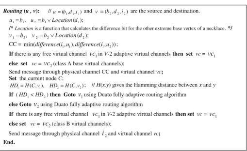
Fig. 2shows the routing algorithm between nodesu¼ ðb1;d1;i1Þandv¼ ðb2;d2;i2Þin pseudo code. Note that the

algo-rithm contains three main steps:

1. Move towards the nearest base neighbor using any of theV-2 adaptive virtual channels. If allV-2 adaptive virtual

chan-nels are busy use the virtual channel of class A from base virtual chanchan-nels to move toward the nearest base neighbor in the source necklace.

2. Move towards the nearest neighbor of the destination using fully adaptive routing algorithm in the hypercube withV-1

virtual channels[12]. If allV-1 virtual channels are busy use the remaining virtual channel with e-cube routing in the base

hypercube.

3. Now the current node is one of the base vertices of the destination necklace. Move towards the destination node using

any of theV-2 adaptive virtual channels. If allV-2 virtual channels are busy use the virtual channel of class B from base

virtual channels to move toward the destination node along the destination necklace.

4. The analytical model

In this section, we derive an analytical performance model for wormhole adaptive routing in a necklace hypercube. Our analysis focuses on the routing algorithm which was introduced in previous section but the modelling approach used here can be equally applied for other routing schemes.

(4)

The measure of interest in our model is theaverage message latencyas a representative for network performance. The fol-lowing assumptions are made when developing the proposed performance model. These assumptions have been widely

used in similar modelling studies[1–5,7,8,14,17,18].

(a) Messages are broken into some packet of fixed length ofMflits. The flit transfer time between any two neighbouring

nodes is assumed to be equal to one cycle.

(b) Message destinations are uniformly distributed across the network nodes.

(c) Nodes generate trafﬁc independently of each other, which follow a Poisson process, with a mean rate ofkgmessages/

cycle.

(d) Messages are transferred to the local processor through the ejection channel once they arrive at their destination.

(e) Vvirtual channels per physical channel are used. These virtual channels are used according to the routing algorithm

described in the previous section.

According to the proposed fully adaptive routing algorithm, a message must cross three sub-networks from the source node to reach the destination node. At ﬁrst, it moves from the source node to the nearest base node; then moves to the near-est base node of the dnear-estination node in the base hypercube; and ﬁnally crosses the dnear-estination necklace to reach the

des-tination node. Therefore, we have 3 message latencies: the mean message latency at the source necklace,LatencyN, the mean

message latency at the base hypercube,LatencyH, and ﬁnally the mean message latency at the destination necklace,LatencyN.

Hence, the total mean message latency can be predicted as:

Latency¼LatencyHþ2LatencyN ð1Þ

In order to compute the mean message latency we must consider three parameters: the mean network latency,S, that is

the time to cross the network, the mean waiting time seen by a message in the source node to be injected into the network, Ws. To model the effect of virtual channels multiplexing, the mean message latency is then scaled by a factor,V, representing

the average degree of virtual channels multiplexing that takes place at a given physical channel[12]. Therefore, the mean

message latency in each sub-network can be approximated as

Latency¼ ðSþWsÞV: ð2Þ

The average number of hops that a message makes across the necklace sub-network,dN, is given by

dN¼ 1 k Xk=2 b c i¼1 2i ð3Þ A value of1

kdk=2emust be addeddN, if the necklace length is odd.

The average number of hops that a message makes across the base cube network,dH, is given by[12]

dH¼

n

2

2n

2n1 ð4Þ

Routing (u , v): //u=( ,b d i₁ ₁, )₁ and v=( ,b d i₂ ₂, )₂ are the source and destination.

1 1, 2 1 ( );1 u =b u = ∨b Location d

/* Location is a function that calculates the difference bit for the other extreme base vertex of a necklace. */

1 2, 2 2 ( 2); v =b v = ∨b Location d

CC =min(difference(i1,u1),difference(i1,u2));

If there is any free virtual channel

vc

₁inV-2 adaptive virtual channels then set vc =

vc

₁

else set vc=

vc

₂(class A base virtual channels);

Send message through physical channel CC and virtual channel vc; Set the current node C;

) , ( ), , ( 1 2 2 1 HCv HD HCv

HD = = ; // H(x,y) gives the Hamming distance between xandy

If (HD1<HD2) then Goto

v

1using Duato fully adaptive routing algorithm

else Goto

v

₂using Duato fully adaptive routing algorithm

If there is any free virtual channel

vc

₁inV-2 adaptive virtual channels then set vc =

vc

₁

else set vc=

vc

₂(class B virtual channels);

Send message through physical channel

i

₂and virtual channel vc; End.

(5)

Fig. 3shows a necklace of (2, 5)-RNH. In this ﬁgure all messages generated in node 3 cross edge (2, 3) except those that their destination is node 1, 2 or 3. If we consider the messages that are generated in node 4 and node 5 and their correspond-ing destinations are nodes 1, 2 and 5 (most crosscorrespond-ing edge (3, 2)) the exact message trafﬁc rate over this edge can be expressed as kg N4 N1þkg 2 N1þkg 1 N1¼kg ð5Þ

We can compute the trafﬁc over edge (2, 1) as follows. All messages generated in node 3 cross edge (2, 1) except those that their destination is node 2, 4 or 5. Also, all messages generated in node 2, for destinations not being node 3, 4 or 5, cross this edge. Considering messages generated in node 4 for node 1, we can write the average trafﬁc rate over this channel as

kg N4 N1þkg N4 N1þkg 1 N1ﬃ2kg ð6Þ

Using a similar approach, the trafﬁc rate over the channels of a necklace with k nodes can be written as

kg;2kg;3kg;. . .;k=2kg. We have similar results for the edges in the other direction[12]. Therefore, we can compute the

aver-age trafﬁc rate received by each necklace channel,kcN, as

kcN¼kg Pk=2 i¼1i k=2 ¼ ðk=2þ1Þ kg 2 ð7Þ

The trafﬁc rate over the edge that connects the last necklace node to the base node isk

2kg. As each base node hasn

neck-laces and the trafﬁc rate generated in a base node itself iskg, we can compute the trafﬁc rate injected to the base hypercube

by a base node as

kb¼kgþn

k

2kg ð8Þ

Fully adaptive routing in the base hypercube allows a message to use any available channel that brings it closer to its destination node, resulting in almost evenly distributed trafﬁc rate over hypercubic channels. A router in the base hypercube

hasnoutput channels. Since each message travels, on averagedhops to cross the network, the rate of messages received by

each hypercubic channel,kcH, can be expressed as[12]

kcH¼

kbN

2ðN1Þ ð9Þ

Let us follow a typical message which makesdhops to reach at its destination. The average network latency,S, seen by the

message crossing from the source to destination node, consists of two parts: one is the time of actual message transmission,

and the blocking time in the network. Therefore,S, can be expressed as

S¼M1þdþdTb ð10Þ

whereMis the message length, andTbis the average blocking time seen by the message at each hop. The termTbis given by

Tb¼Pblockw ð11Þ

withPBlockbeing the probability that a message is blocked at the current channel andwis the mean waiting time to acquire a channel in the event of blocking. A message is blocked at a given channel in the necklace sub-network when all adaptive and

deterministic virtual channels of the current physical channel are busy. LetPabe the probability that all adaptive virtual

channels of a physical channel are busy andPa&ddenote the probability that all adaptive and deterministic virtual channels

of a physical channel are busy. In necklace sub-networks, we have only one path for the messages, so no adaptivity exists for messages moving across a necklace.

In order to computePa&dN (probabilityPa&dfor necklaces), we must consider two cases:

(a) The probability that all ofVvirtual channels of a physical channel are busy,PV, and

(b) the probability thatV-1 virtual channels of theVvirtual channels associated to a physical channel are busy. In this case

only one combination ofV-1 virtual channels of the totalVvirtual channels can result in blocking.

0 1 2 3 4 1 2 3 4 5 7 5 7 Fig. 3.A (2, 5)-RNH network.

(6)

So, the probability that all adaptive and deterministic virtual channels of a physical channel are busy can be expressed as Pa&dN ¼PVþ PV1 V V1 _ð₁₂_Þ

In order to compute the probability of blocking,Pblock, we average over all the probabilities that a message may be blocked

crossingdhops in the network as

PblockN ¼ 1 dN X dN i¼1 Pa&dN ð13Þ

A message is blocked at a given channel in the hypercube network when all the adaptive virtual channels of the remaining dimensions to be visited and also the deterministic virtual channel of the current dimension are busy. We can then write Pa_H;Pa&dH andPblockH as[12]:

PaH¼PVþ PV1 V V1 ð14Þ Pa&dH ¼PV ð15Þ PblockH ¼ 1 dH X dH1 i¼0 PaH dHi1_P a&dH ð16Þ

wheredHis the average number of hops that a message might take in the hypercube sub-network.

To determine the mean waiting time,w, to acquire a virtual channel when a message is blocked, a physical channel is

treated as an M/G/1 queue with a mean waiting time of[9]

w¼

q

S1þC2_S 2ð1

q

Þ ð17Þ

q

¼kcS ð18Þ C2_S¼

r

2 S S2 ð19Þ

wherekcis the trafﬁc rate on the channel (given by Eqs.(7) or (9)for necklace or hypercubic channels), is its service time

calculated by Eq.(10), and is the variance of service time distribution. Since the minimum service time at a channel is equal

to the message length,M, following a suggestion given in[5], the variance of the service time distribution can be

approxi-mated as. Hence, the mean waiting time becomes

w¼kcS

2_ð₁_{þ ð}₁_M=S_Þ2 Þ

2ð1kcSÞ

ð20Þ

Similarly, modelling the local queue in the source node as an M/G/1 queue, with the mean arrival ratekg=Vand service

timeSwith an approximated varianceðSMÞ2, yields the mean waiting time seen by a message at the source node as[12]

Ws¼ kg vS 2_ð₁_{þ ð}₁_M=S_Þ2 Þ 2ð1kg VSÞ ð21Þ

The probability,Pv, thatvvirtual channels are busy at a physical channel can be determined using a Markovian model. Let

state

p

vð06v6VÞcorrespond tovvirtual channels being busy. The transition rate out of state

p

vto state

p

vþ1 is the trafﬁc

ratekc(given by Eqs.(7) and (9)) while the rate out of state

p

vto state

p

v1is ( is given by Eq.(10)). The transition rates out of

state

p

vare reduced bykcto account for the arrival of messages while a channel is in this state.

The Markovian model results in the following steady state probability[4], in which the service time of a channel has been

approximated as the network latency of that channel, as

Pv¼ ð

1kcSÞðkcSÞv; 06v<V

ðkcSÞv; v¼V:

(

ð22Þ When multiple virtual channels are used per physical channel, they share the physical bandwidth in a time-multiplexed manner. The average degree of multiplexing of virtual channels, that takes place at a given physical channel, can then be

estimated by[4] V¼ PV v¼1v2pv PV v¼1vpv : ð23Þ

(7)

The above equations reveal that there are several inter-dependencies between the different variables of the model. For

instance, Eqs.(10) and (11)reveal that Sis a function ofwwhile Eq.(17) shows thatw is a function ofS. Given that

closed-form solutions to such inter-dependencies are very difﬁcult to determine, the different variables of the model are

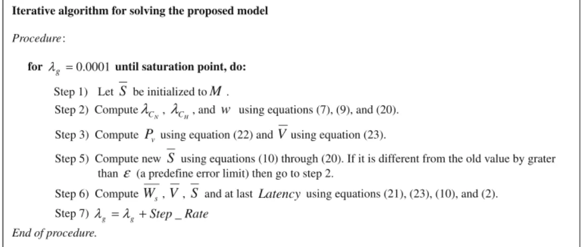
computed using an iterative technique.Fig. 4shows different steps of the iterative algorithm.

5. Validation of the model

The proposed analytical model has been validated through a discrete-event simulator (Xmulator[15]) that mimics the

behaviour of the described routing algorithms in the necklace hypercube at flit level. The simulator uses the same assump-tions as the analysis, and some of these assumpassump-tions are detailed here with a view to making the network operation clearer. The network cycle time is defined as the transmission time of a single flit from one router to the next. Messages are

gener-ated at each node according to a Poisson process with a mean inter-arrival rate ofkgmessages/cycle. Message length is ﬁxed

atMﬂits. Destination nodes are determined using a uniform random number generator. The mean message latency is

de-fined as the mean amount of time from the generation of a message until the last data flit reaches the local processor at the destination node. The other measures include the mean network latency, the time taken to cross the network, the mean queuing time at the source node, and the time spent at the local queue before entering the first network channel. Numerous validation experiments have been performed for several combinations of network sizes, message lengths, and number of vir-tual channels to validate the model.

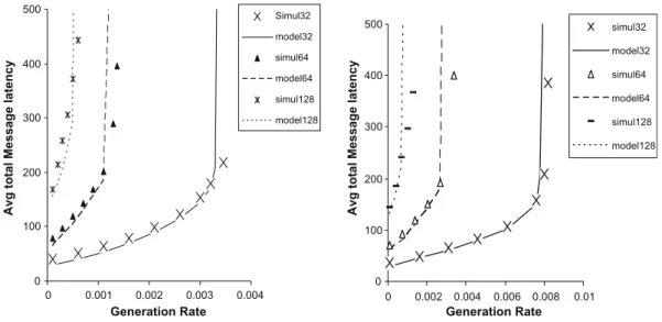
Figs. 5–8depict latency results predicted by the model explained in the previous section plotted against those provided by the simulator for different scenarios. The horizontal axis in the ﬁgure shows the trafﬁc generation rate at each node while

the vertical axis shows the mean message latency. InFig. 5, we consider two very large networks with more than 10,000. We

consider 10 virtual channels per physical channel, and two different message lengths ofM= 32 and 64 ﬂits (larger message

size, e.g. 128 ﬂits, took the network to saturation state for small values of trafﬁc generation rates). InFig. 6, we consider two

large networks (more than 1000 nodes) withV= 8 virtual channels per physical channel, and three different message lengths

ofM= 32, 64 and 128 ﬂits.Fig. 7represents the same results for medium sized networks (about 256 nodes); here, we use

V= 6 virtual channels per physical channel and message lengthM= 32, 64 and 128 ﬂits. Finally, inFig. 8, we have shown

a comparison between the results given by the model and those gathered from the simulation experiments for two small

networks (about 100 nodes); here the number of virtual channels isV= 4 per physical channel and message length is

M= 32, 64 and 128 ﬂits.

The figures reveal that in all cases the analytical model can predict the mean message latency with a good degree of accu-racy in the steady-state regions. Moreover, model predictions are still good even when the network operates in the heavy traffic region, and when it starts to approach the saturation region. However, some discrepancies around the saturation point are apparent. These can be accounted for by the approximations made to ease the derivation of different variables of the model, e.g. the approximation made to estimate the variance of the service time distribution at a channel. Such an approx-imation greatly simplifies the model as it allows us to avoid computing the exact distribution of the message service time at a given channel, which is not a straightforward task due to inter-dependencies between service times at successive channels as wormhole routing relies on a blocking mechanism for flow control.

6. Analytical performance comparison of hypercubes and necklace hypercubes

In this section, we compare the performance of the necklace hypercube with its equivalent hypercube network. We use

Boura’s model[2]to predict hypercube’s behaviour and the proposed model here to predict the performance of equivalkent

Iterative algorithm for solving the proposed model

Procedure:

for λg =0.0001 until saturation point, do: Step 1) Let

S

be initialized to

M

. Step 2) Compute N C

λ

, H C

λ

, and

w

using equations (7), (9), and (20). Step 3) Compute

P

v using equation (22) and

V

using equation (23).

Step 5) Compute new

S

using equations (10) through (20). If it is different from the old value by grater than

ε

(a predefine error limit) then go to step 2.

Step 6) Compute

W

s,

V

,

S

and at last

Latency

using equations (21), (23), (10), and (2). Step 7) λg = λg+Step_Rate

End of procedure.

(8)

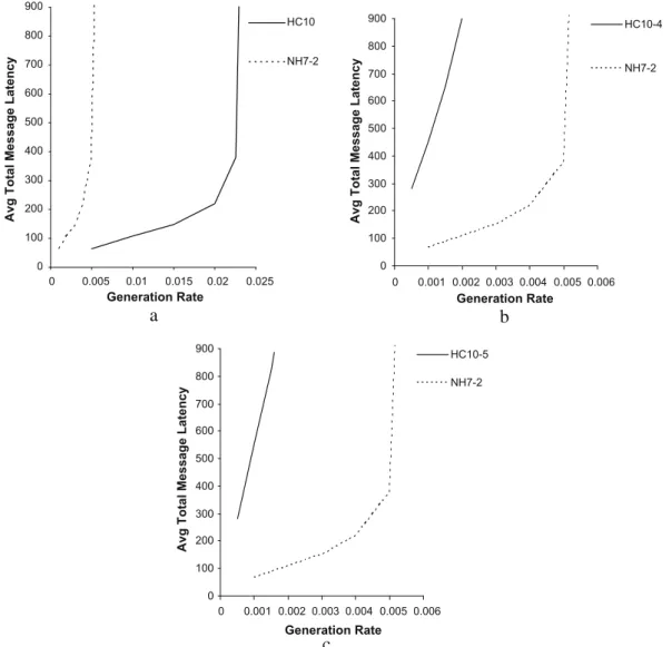
necklace hypercubes. We first compare the networks with equal number of nodes without considering any technological or implementation constraint. To do so, we consider a 10-dimensional hypercube and a (7, 2)-RNH, both with 1024 nodes. Fig. 9a shows the average message latency of these networks when message size is fixed atM= 64 flits and number of virtual

channels per physical channel isV= 8. As can be seen in the ﬁgure, the hypercube performs better than the equivalent

neck-lace network. One reason is the excessive number of channels existing in the hypercube which enables the network to

tol-erate higher trafﬁc rates. Moreover, the average distance for theðn;kÞ-RNH issþt

2, where s¼4vþn 2_k 2ð2þnkÞ; v¼ nþ1 8 ðk 2 þkþ1Þ þ1 2; if nisodd n 8ðk 2 þ2kþkmod 2Þ; if niseven ( ; t¼ ðk2Þðkþ1Þðkþ3Þ 4 n 2 ; ifkisodd ðk2Þðkþ2Þ2 4 n 2 ; ifkiseven 8 > > > > > > < > > > > > > : ð24Þ 0 100 200 300 400 500 600 0 0.001 0.002 0.003 Generation Rate

Avg Total Message Latency Avg Total Message Latency Simul32 Model32 Simul64 Model64 Simul128 Model128 0 100 200 300 400 500 0 0.002 0.004 Generation Rate Simul32 Model32 Simul64 Model64 Simul128 Series6

Fig. 6.The average message latency predicted by the model against simulation results when eight virtual channels are used per physical channel and message length isM= 32, 64, 128 ﬂits, in (7, 8)-RNH (left) and (7, 3)-RNH (right) networks.

0 100 200 300 400 500 600 700 800 900 0 0.0002 0.0004 0.0006 0.0008 0.001 Generation Rate Simul32 Model32 Simul64 Model64 0 200 400 600 800 1000 1200 0 5E-05 0.0001 0.0002 0.0002 0.0003 Generation Rate

Avg Total Message Latency

Simul32 Model32 Simull64 Model64

Fig. 5.The average message latency predicted by the model against simulation results when 10 virtual channels are used per physical channel and message length isM= 32, 64 ﬂits, in (10, 6)-RNH (left) and (10, 3)-RNH (right) networks.

(9)

Comparing it to the average distance in a binary n-cube (i.e. n/2) reveals a big difference especially when the necklace

size,k, is big.

When an interconnection network is implemented on a chip or over a board, the bisection bandwidth has the most

important effect on the performance. Thus, many studies, e.g.[1,18], consider a constant bisection bandwidth when

compar-ing two equivalent networks (with the same number of nodes). Accordcompar-ing to[1], the multiplication of bisection width of the

network (the number of edges to be cut in order to halve the network in two equivalent parts) and channel bandwidth is

deﬁned to be the bisection bandwidth of the network. The bisection width of the hypercube is equal to 2n1_{, and the}

bisec-tion width of them-dimensional necklace hypercube is 2m[19]. Assuming two equivalent networks, a hypercube with

bisec-tion width ofBWH and channel bandwidth ofCWH, and a necklace hypercube with bisection widthBWNH and channel

bandwidth ofCWNH, and considering a ﬁxed network bisection bandwidth, we can write

BWHCWH¼BWNHCWNH ð25Þ

Thus, the ﬂit size of the hypercube equalsBWNH

BWH CWNH. So, considering that the phit size of the necklace hypercube equals

its ﬂit size, the transmission time for a ﬂit in the equivalent hypercube will beBWH

BWNHtimes of the ﬂit transmission time in the

necklace hypercube. 0 100 200 300 400 500 0 0.001 0.002 0.003 0.004 Generation Rate Simul32 model32 simul64 model64 simul128 model128 0 100 200 300 400 500 0 0.002 0.004 0.006 0.008 0.01 Generation Rate

Avg total Message latency

simul32 model32 simul64 model64 simul128 model128

Fig. 7.The average message latency predicted by the model against simulation results when six virtual channels are used per physical channel and message length isM= 32, 64, 128 ﬂits, in (4, 8)-RNH (left) and (4, 3)-RNH (right) networks.

0 100 200 300 400 500 0 0.002 0.004 0.006 Generation Rate

Avg Total Message Latency Avg Total Message Latency Simul32 Model32 Simul64 Model64 Simul128 Model128 0 50 100 150 200 250 300 350 400 450 0 0.005 0.01 0.015 Generation Rate Simul32 Simul64 Simul128 Model32 Model64 Model128

Fig. 8.The average message latency predicted by the model against simulation results when four virtual channels are used per physical channel and message length isM= 32, 64, 128 ﬂits, in (2, 8)-RNH (left) and (2, 3)-RNH (right) networks.

(10)

Fig. 9b compares the performance of the 10-dimensional hypercube and (7, 2)-RNH under constant bisection bandwidth

constraint. The message length is ﬁxed at 64 ﬂits and the number of virtual channels per physical channel isV= 8. As can be

seen in this ﬁgure, the necklace hypercube outperforms the equivalent hypercube under bisection bandwidth constraint. Pin-out constraint also has an important impact on the performance, when an interconnection network is implemented

by wiring between chips, boards, and cabinets[1]. Constant pin-out constraint has been already used by other researchers

[1,18]for comparing different networks. Pin-out of a node is deﬁned to be the node degree (the number of channels in a

node) multiplied by the channel width. Assuming two equivalent networks, a hypercube with node degreePHand channel

width ofCWH, and a necklace hypercube with bisection widthPNHand channel width ofCWNH, and considering pin-out

con-straint, we can write

PHCWH¼PNHCWNH ð26Þ

Using Eq.(26), we can calculate the ratio between the ﬂit transmission time for the hypercube and necklace hypercube.

The node degree in an n-dimensional hypercube isn, but there is a problem when we want to determine the pin-out of

neck-lace hypercube. Here, we have two types of nodes: neckneck-lace nodes with degree of 2 and the hypercube nodes with degree of 2n. As the number of nodes with degree 2 is much larger than those with degree 2n, we can use the approximate value of 2 for node degree.

Fig. 9c shows the performance comparison of the 10-dimensional hypercube and (7, 2)-RNH under pin-out constraint. As depicted in the ﬁgure, the necklace hypercube performs better than the hypercube under pin-out constraint.

0 100 200 300 400 500 600 700 800 900 0 0.005 0.01 0.015 0.02 0.025 Generation Rate

Avg Total Message Latency Avg Total Message Latency

Avg Total Message Latency

HC10 NH7-2 0 100 200 300 400 500 600 700 800 900 0 0.001 0.002 0.003 0.004 0.005 0.006 Generation Rate HC10-4 NH7-2

a

0 100 200 300 400 500 600 700 800 900 0 0.001 0.002 0.003 0.004 0.005 0.006 Generation Rate HC10-5 NH7-2

c

b

Fig. 9.The average message latency predicted by the model for a 10 dimensional hypercube and (7, 2)-RNH when eight virtual channels are used per physical channel and message length isM= 64, when (a) no constraints is considered, (b) under bisection bandwidth constraint, and (c) under pin-out constraint.

(11)

7. Conclusion and future work

The necklace hypercube network has recently been introduced as an attractive alternative to the well-known hypercube. In this paper, we introduced a mathematical performance model of adaptive wormhole routing in necklace hypercubes and validated it through simulation experiments. We saw that the proposed model manages to achieve a good degree of accuracy while maintaining simplicity, making it a practical evaluation tool that can be used by the researchers in the ﬁeld to gain insight into the performance behaviour of fully adaptive routing in wormhole-switched necklace hypercube.

We then used the proposed analytical model to compare the performance of same-sized necklace hypercubes and hyper-cubes with and without implementation constraints. The considered implementation constraints were the bisection band-width and pin-out. When no implementation constraints were taken into account, the hypercube was shown to behave better than its equivalent necklace hypercube. However, under both bisection bandwidth and pin-out implementation con-straints the necklace hypercube outperformed its equivalent hypercube.

Our next objective is to analyse the performance of the necklace hypercube under important non-uniform trafﬁc patterns. Examining other types of necklace networks, with different base networks, can also be another line of research for future work. Considering and analyzing irregular necklace networks can be another interesting research topic. Another network

which is based on the hypercube and is very similar to necklace hypercube, is thestretched hypercube[20]. Conducting

sim-ilar analytical studies for this network can be another line of future research. References

[1] A. Agarwal, Limits on interconnection network performance, IEEE Transactions on Parallel and Distributed Systems 2 (1991) 398–412.

[2] Y. Boura, C.R. Das, T.M. Jacob, A performance model for adaptive routing in hypercubes, in: Proceedings of the International Workshop on Parallel Processing, 1994, pp. 11–16.

[3] B. Ciciani, M. Colajanni, C. Paolucci, An accurate model for the performance analysis of deterministic wormhole routing, in: Proceedings of the 11th International Parallel Processing Symposium, 1997, pp. 353–359.

[4] W.J. Dally, Virtual channel ﬂow control, IEEE Transactions on Parallel and Distributed Systems 3 (1992) 194–205.

[5] J.T. Draper, J. Ghosh, A comprehensive analytical model for wormhole routing in multicomputer systems, Journal of Parallel and Distributed Computing 23 (1994) 202–214.

[6] J. Duato, S. Yalamanchili, L. Ni, Interconnection Networks: An Engineering Approach, Morgan Kaufmann, 2005.

[7] R. Greenberg, L. Guan, Modelling and comparison of wormhole routed mesh and torus networks, in: Proceedings of the 9th IASTED International Conference on Parallel and Distributed Computing and Systems, 1997, pp. 501–506.

[8] J. Kim, C.R. Das, Hypercube communication delay with wormhole routing, IEEE Transactions on Computers 43 (1994) 806–814. [9] L. Kleinrock, Queueing Systems, vol. 1, John Wiley, 1975.

[10] S. Meraji, H. Sarbazi-Azad, Performance evaluation of deterministic routing in wormhole necklace cubes, in: Proceedings of the ACS/IEEE Conference on Computers and Applications, Amman, Jordan, 2007.

[11] S. Meraji, A. Nayebi, H. Sarbazi-Azad, Performance evaluation of adaptive wormhole routing in necklace hypercubes, in: International Conference on Computing: Theory and Applications, IEEE Press, Kolkata, India, March 5–7, 2007.

[12] S. Meraji, Performance evaluation of necklace hypercube interconnection networks, M.Sc. Thesis, Sharif University of Technology, October 2006. [13] S. Meraji, H. Sarbazi-Azad, A. Patooghy, Performance modeling of necklace hypercubes, in: 6th International Workshop on Performance Modeling,

Evaluation, and Optimization of Parallel and Distributed Systems (PMEO-PDS 2007), held in Conjunction with IEEE IPDPS2007, Long Beach, CA, USA, 26–30 March 2007.

[14] H. Hashemi-Najafabadi, H. Sarbazi-Azad, P. Rajabzadeh, An accurate performance model of fully adaptive routing in wormhole-switched 2D-mesh multicomputers, Microprocessors and Microsystems 31 (2007) 445–455.

[15] A. Nayebi, S. Meraji, A. Shamaei, H. Sarbazi-Azad, Xmulator: a listener-based integrated simulation platform for interconnection networks, in: Proceedings of Asia Modelling Symposium, IEEE Press, Thailand, 2007.

[16] A. Patel, A. Kusalik, C. McCrosky, Area-efﬁcient VLSI layout for binary hypercubes, IEEE Transactions on Computers 49 (2000) 160–169.

[17] H. Sarbazi-Azad, M. Ould-Khaoua, L.M. Mackenzie, An accurate analytical model of adaptive wormhole routing in k-ary n-cube interconnection networks, Performance Evaluation 43 (2001) 165–179.

[18] H. Sarbazi-Azad, Constraint-based performance comparison of multi-dimensional interconnection networks with deterministic and adaptive routing strategies, Journal of Computers and Electrical Engineering 30 (2004) 167–182.

[19] P. Shareghi, H. Sarbazi-Azad, Topological properties of necklace networks, in: IEEE International Symposium on Parallel Architectures, Algorithms and Networks (IEEE I-SPAN), IEEE Computer Society Press, 2005, pp. 40–45.

[20] P. Shareghi, H. Sarbazi-Azad, The stretched network: properties, routing, and performance, Journal of Information Science and Engineering 24 (2008) 361–378.